International Journal for Quality Research 8(3) 399-416 ISSN 1800-6450
Yerriswamy Wooluru
1Swamy D.R.
P. Nagesh
Article info: Received 22.03.2014 Accepted 20.06.2014 UDC – 54.061
THE PROCESS CAPABILITY ANALYSIS - A
TOOL FOR PROCESS PERFORMANCE
MEASURES AND METRICS - A CASE STUDY
Abstract: Process Capability can be evaluated through the computations of various process capability ratios and indices. The basic three capability indices commonly used in manufacturing industries are Cp, Cpk,Cpm and Cpmk .Process capability indices are intended to provide single number assessment of the ability of a process to meet specification limits on quality characteristics of interest. Thus, it identifies the opportunities for improving quality and productivity. The level of significance on process capability analysis has been increased considerably over last decade, but the literature findings reveal the importance of understanding the concepts, methodologies and critical assumptions while its implementation in manufacturing process. The objective of this paper is to conduct process capability analysis for boring operation by understanding the concepts, methodologies and making critical assumptions.
Keywords: Process Capability Index, Normal Distribution, Statistical Process Control, Run chart
1.
Introduction
1Process capability study is a method of combining the statistical tools developed from the normal curve and control charts with good engineering judgment to interpret and analyze the data representing a process. The purpose of the process capability study is to determine the variation spread and to find the effect of time on both the average and the spread. The administration, analysis and use of the process capability study should be an integral part of the quality engineering function. The results could be used for new design applications, inspection planning and evaluation techniques. It is a
1
Corresponding author: Yerriswamy Wooluru email: [email protected]
type of tool that can be used to prevent defects during the production cycle through better designs, through factual knowledge of machine or process limitations and through knowledge of process factors that can or cannot be controlled. In any manufacturing operation there is a variability which is manifested in the product made by the operations .Quantifying the variability with objectives and advantages of reducing it in the manufacturing process is the prime activity of the process management.
Process Capability refers to the evaluation of how well a process meets specifications or the ability of the process to produce parts that conform to engineering specifications, Process Control refers to the evaluation of process stability over time or the ability of the process to maintain a state of good statistical control. These are two separate but
vitally important issues that we must address when considering the performance of a process and so the assessment of process capability is inappropriate and statistically invalid to assess with respect to conformance to specifications without being reasonably assured of having good statistical control. Before evaluating the process capability, the process must be shown under statistical control i.e. the process must be operating under the influence of only chance causes of variation and also ensure that the process data is normally distributed and observations are independent.
A process may produce a large number of pieces that do not meet the specifications, even though the process itself is in a state of statistical control (i.e., all the points on the X-bar and R charts are within the 3 sigma limits and vary in random manner).This may be due to the lack of centering of the process mean in other words, the actual mean value of the parts being produced may be significantly different from the specified nominal value of the part. If this is the case, an adjustment of the machine to move the mean closer to the nominal value may solve the problem. Another possible reason for lack of conformance to specifications is that a statistically stable process may be producing parts with an unacceptably high level of common-cause variation, even though the process is centered at the nominal value.
2.
The basic capability indices
commonly used in
manufacturing industries are
Cp, Cpk Cpm and Cpmk.
Cp: It simply relates the Process Capability to the Specification Range and it does not relate the location of the process with respect to the specifications. Values of Cp exceeding 1.33 indicate that the process is adequate to meet the specifications. Values of Cp between 1.33 and 1.00 indicate that the process is adequate to meet specifications
but require close control. Values of Cp below 1.00 indicate the process is not capable of meeting specifications. If the process is centered within the specifications and is approximately “normal” then Cp = 1.00 results in a fraction nonconforming of 0.27%. It is also known as process potential. Cpl: It estimates process capability for specifications that consist of a lower limit only (for example, strength) and it assumes process output is approximately normally distributed. Cpu: It estimates process capability for specifications that consist of an upper limit only (for example, concentration). Assumes process output is approximately normally distributed.
Cpk: It considers process average and evaluates the process spread with respect to where the process is actually located. The magnitude of Cpk relative to Cp is a direct
measurement of how off-centre the process is operating. It assumes process output is approximately normally distributed. If the characteristic or process variation is centered between its specification limits, the calculated value for CPK is equal to the
calculated value for CP. But as soon as the
process variation moves off the specification center, it is penalized in proportion to how far it‟s offset. CPK is very useful and very
widely used. Generally, a CPK greater than
1.33 indicates that a process is capable in the short term. Values less than 1.33 tells that the variation is either too wide compared to the specification or that the location of the variation is offset from the center of the specification. It may be a combination of both width and location. Cpk measures how far the process mean is from the nearer specification limit in terms of 3σ distances. Cpk works well only for the bell-shaped “normal” (Gaussian) distribution. For others it is an approximation. Cpk = Cp only when the process is perfectly centered. Cp represents the highest possible value for Cpk.
Cpm: It estimates process capability around a target T, it is always greater than zero and
assumes process output is approximately normally distributed. It is also known as the Taguchi capability index, introduced in 1988. Cpk measures how well the process mean is centered within the specification limits, and what percentage of product will be within specification limits. Instead of focusing on specification limits, Cpm focuses on how well the process mean corresponds to the process target, which may or may not be midway between the specification limits. Cpm is motivated by Taguchi‟s “Loss Function”. The denominator of Cpm includes the Root Mean Square deviation from the target. Cpk is preferred to Cp because it measures both process location and process standard deviation. Cpm is often preferred to Cpk because the variability term used in the index
is more consistent with Run to Target Philosophy.
Cpmk: It estimates process capability around a target (T), and accounts for an off-center process mean and assumes process output is approximately normally distributed. The process capability index - Cpk considers
process average and evaluates half the process spread with respect to where the process average is actually located, though Cpk takes the process mean into consideration
but it fails to differentiate an on-target process from off-target process. The way to address this difficulty is to use a process capability index Cpm that is better indicator of centering.
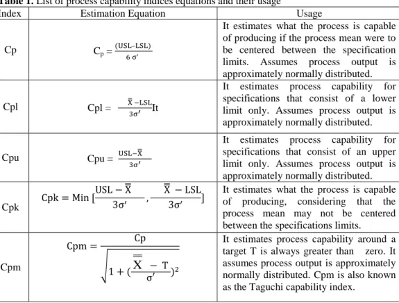
Summary of Process Capability Indices and their usage is presented in the Table 1.
Table 1. List of process capability indices equations and their usage
Index Estimation Equation Usage
Cp Cp =
–
It estimates what the process is capable of producing if the process mean were to be centered between the specification limits. Assumes process output is approximately normally distributed.
Cpl Cpl = ̿ It
It estimates process capability for specifications that consist of a lower limit only. Assumes process output is approximately normally distributed.
Cpu Cpu = ̿
It estimates process capability for specifications that consist of an upper limit only. Assumes process output is approximately normally distributed.
Cpk
̿
̿
It estimates what the process is capable of producing, considering that the process mean may not be centered between the specifications limits.
Cpm
√
X
It estimates process capability around a target T is always greater than zero. It assumes process output is approximately normally distributed. Cpm is also known as the Taguchi capability index.
Cpmk
√
X
It estimates process capability around a target T and accounts for an off-center process mean. Assumes process output is approximately normally distributed.
3.
Methodology
Estimation of Process Capability for boring operation involves the following steps:
Understanding the basic concepts of process capability analysis and its measures.
Process data collection.
Calculate required statistics
Validate the critical assumptions.
Estimation of Cp, Cpu, Cpl, Cpk, Cpm and Cpmk.
Analysis of process capability results.
If the process is not capable of meeting the specification, find the predominant factor that affecting the process capability.
Take action to improve the process performance.
Estimate the confidence intervals and Carryout Hypothesis Testing.
4.
Data collection
Critical quality characteristic of the gear i.e. Bore diameter on the driver gear processed by boring operation in an automotive industry has been identified.The product description is given in the Table 2 and the measured values are presented in the Table 3.
Table 2. Product description
Material: Cast steel Part Name : Driver Gear Operation: Boring Specifications: 205.00 ± 0.05 Instrument used : Dial Bore Gauge All dimensions are in “ mm”
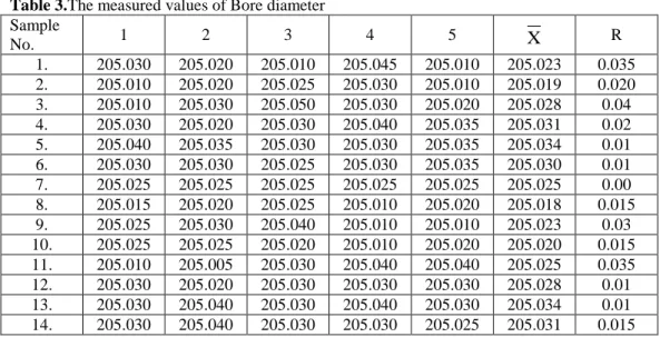
Table 3.The measured values of Bore diameter Sample
No. 1 2 3 4 5
X
R1. 205.030 205.020 205.010 205.045 205.010 205.023 0.035 2. 205.010 205.020 205.025 205.030 205.010 205.019 0.020 3. 205.010 205.030 205.050 205.030 205.020 205.028 0.04 4. 205.030 205.020 205.030 205.040 205.035 205.031 0.02 5. 205.040 205.035 205.030 205.030 205.035 205.034 0.01 6. 205.030 205.030 205.025 205.030 205.035 205.030 0.01 7. 205.025 205.025 205.025 205.025 205.025 205.025 0.00 8. 205.015 205.020 205.025 205.010 205.020 205.018 0.015 9. 205.025 205.030 205.040 205.010 205.010 205.023 0.03 10. 205.025 205.025 205.020 205.010 205.020 205.020 0.015 11. 205.010 205.005 205.030 205.040 205.040 205.025 0.035 12. 205.030 205.020 205.030 205.030 205.030 205.028 0.01 13. 205.030 205.040 205.030 205.040 205.030 205.034 0.01 14. 205.030 205.040 205.030 205.030 205.025 205.031 0.015
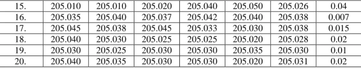
15. 205.010 205.010 205.020 205.040 205.050 205.026 0.04 16. 205.035 205.040 205.037 205.042 205.040 205.038 0.007 17. 205.045 205.038 205.045 205.033 205.030 205.038 0.015 18. 205.040 205.030 205.025 205.025 205.020 205.028 0.02 19. 205.030 205.025 205.030 205.030 205.035 205.030 0.01 20. 205.040 205.035 205.030 205.030 205.020 205.031 0.02
5.
Process Capability Analysis
According to Kotz and Montgomery (2000) the following critical assumptions have been made and validated before estimating the process capability for boring operation.
The process must be in state of statistical control.
The quality characteristic has a normal distribution.
In the case of two sided specifications, the process mean is centered between the lower and upper specification limits.
Observations must be random and independent of each other.
All the above assumptions have been verified as follows.
5.1 Construction of ̅ and R- Chart to assess the statistical stability of the boring operation
Control limits for ̅ - Chart
̿ ̅ 205.049 + [(0.577) (0.029)] =205.06560,
̿ ̅ = 205.049 - [(0.577) (0.029)] =205.03219
Control limits for R-Chart
UCL= ̅= 2.114 x0.029 =0.06124 LCL= ̅ = 0.00 x0.029=0.0000 From Table, for n=5 .
. =0.00. =2.114
It has been observed from the Figure 1 that all plotted sample range and mean values are within the control limits on both R-Chart as well as X-Bar chart and no indication of Trend, shift, run and clustering has been noticed. Hence, it is concluded that the process is under statistical control and operating under the influence of only chance causes of variation. i.e., the process is stable over time.
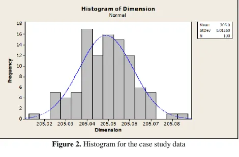
5.2 Normal probability plot and histogram for validating the Normality assumption
Graphical methods including the histogram and normal probability plot are used to check the normality of the case study data. Figure 2 displays the histogram and Figure 3 display the normal probability plot for the case study data. The sample data appears to be normal.
Figure 2. Histogram for the case study data
Test results for normal probability plot for the data from MINITAB -14 statistical software output shows Mean: 205.00, Standard deviation: 0.0126, Anderson Darling test statistic value: 0.215 and P- value: 0.844 is greater than the significance level (𝛼 = 0.05) implies that the data is
distributed normally .Thus, it is concluded that the sample data can be regarded as taken from a normal process.
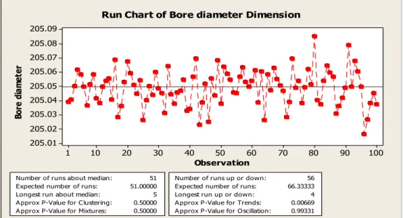
5.3 Construction of Run chart for checking the assumption of Randomness using MINITAB software
Observation Bo re d ia m et er 100 90 80 70 60 50 40 30 20 10 1 205.09 205.08 205.07 205.06 205.05 205.04 205.03 205.02 205.01
Number of runs about median:
0.50000 51 Expected number of runs: 51.00000 Longest run about median: 5 Approx P-Value for Clustering: 0.50000 Approx P-Value for Mixtures:
Number of runs up or down:
0.99331 56 Expected number of runs: 66.33333 Longest run up or down: 4 Approx P-Value for Trends: 0.00669 Approx P-Value for Oscillation:
Run Chart of Bore diameter Dimension
Figure 4. Run chart for case study data Interpreting the Run Chart: p - values for
clustering, mixtures and oscillation are greater than 𝛼 value of 0.05. In case of the trend, P-value is smaller than the alpha value and it warns that the process is about to go out of control due to the factor like worn tool. The actual numbers of runs are close to the expected number of runs. Hence it is concluded that the observations in the data set are random. After validating the three critical assumptions, the process capability for the boring operation would be quantified.
6.
Estimation of Process
Capability Indices for existing
process conditions
6.1Process Capability Index - Cp
The Average of Averages of the samples (
X
= µ) and Average Range (R
) value are computed. The process standard deviation is obtained with the help of formula, σ‟ =R
/ d2, value of d2 for a sample size of five isnoted as 2.326 from statistical tables for control chart constants.
The process standard deviation (σ‟) =
R
/ d2. σ' = 0.029 / 2.326 = 0.01246.Process capability index, Cp =
–
= 1.34 Percentage ofspecification band used by the current process.
Cr = (1 / Cp) x 100 = (1/ 1.34) x 100 = 74.62
%.This means that the manufacturing process uses 74.62 % of specification band. The capability Ratio
(CR) = =
= 0.744 At present the specification range used by the process is 74.4%.
6.2 Process capability index – Cpk (Second- generation capability index, developed from the original Cp)
( ̿ ̿ ) Cpk = Min
(
) Cpk = Min Therefore, Cpk = 0.026
6.3. Process capability index- Cpm (Second- generation capability index, developed from the original Cp)
√
X
= 0.33
Where, USL and LSL are upper and lower specification limits.‟ is process standard deviation, ̿ is process mean, T is target value.
6.4 Cpmk Process capability index-Cpmk (a third- generation capability index that incorporates the features of Cpk and Cpm).
√
X
= 0.0063
The case study analysis reveals that Cp is not
equal to Cpk which implies that the process is
not exactly centered. Also, Cp, CpkCpm and Cpkmare not very nearer in their magnitude and hence it can be stated that process under study is not exactly centered. It is noticed that even process is under statistical control ,stable over time and have potential to meet the given specification limits, there has been rejections as large as 4,64,626.00 products out of 1 million products due to the shift of the process mean towards upper specification limit as shown in figure 9. In order to reduce the scrap, it is necessary to shift the process mean as close as possible to the target value (i.e., 205.00 mm).
7.
Process capability evaluation
after shifting the process mean
to the specification mean
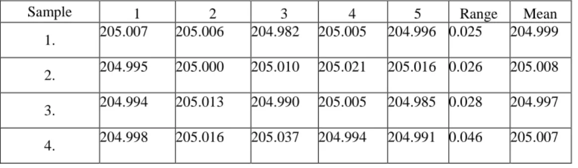
After adjusting the process mean to the target value of 205.00, data was collected and presented in the Table 4.
Table 4. Measured values of bore dia after adjusting the process mean
Sample 1 2 3 4 5 Range Mean
1. 205.007 205.006 204.982 205.005 204.996 0.025 204.999 2. 204.995 205.000 205.010 205.021 205.016 0.026 205.008 3. 204.994 205.013 204.990 205.005 204.985 0.028 204.997 4. 204.998 205.016 205.037 204.994 204.991 0.046 205.007
ΣR=0.66, ̅ =0.033, Σ ̅ = 4100.03, ̿ =205.001
8.
Process capability evaluation
after adjusting the process mean
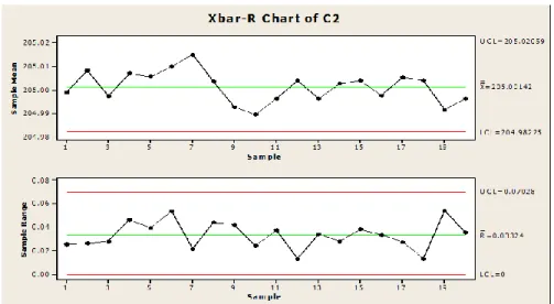
8.1 Construction of ̅ and R- Chart to assess the stability and uniformity of the process
Control limits for ̅ –Chart
̿ ̅ 205.001 + [(0.577)
(0.033)] =205.020
̿ ̅ = 205.001 - [(0.577) (0.033)] =204.982
Control limits for R-Chart
UCL= ̅= 2.114 x0.033 =0.070, LCL= ̅ = 0.00 x0.033=0.0000 From table, n=5 . . =0.00. =2.114
5. 205.019 204.994 205.022 204.983 205.011 0.039 205.006 6. 204.993 205.038 205.028 205.007 204.985 0.053 205.010 7. 205.005 205.015 205.019 205.010 205.026 0.021 205.015 8. 204.985 204.983 205.027 205.005 205.019 0.044 205.004 9. 204.982 204.985 204.982 204.990 205.024 0.042 204.993 10. 204.997 204.987 204.997 204.994 204.973 0.024 204.990 11. 204.986 205.020 204.983 204.993 205.000 0.037 204.996 12. 204.998 205.004 205.007 205.011 205.001 0.013 205.004 13. 204.983 205.017 205.001 204.995 204.985 0.034 204.996 14. 204.986 205.012 205.006 205.014 204.996 0.028 205.003 15. 205.014 204.982 204.998 205.020 205.007 0.038 205.004 16. 205.001 205.013 204.994 205.001 204.980 0.033 204.998 17. 205.020 205.009 204.993 204.995 205.010 0.027 205.005 18. 205.000 205.013 205.001 205.003 205.005 0.013 205.004 19. 204.991 205.017 204.996 204.963 204.992 0.054 204.992 20. 205.015 204.988 205.006 204.980 204.992 0.035 204.996
Figure 5. Control charts for case study data It has been observed that all the plotted
sample range and mean values are within the control limits on both R-Chart as well as X-Bar chart and there are no indications of Trend, shift, run and clustering. Hence it is concluded that the process is under statistical control and operating under the influence of only chance causes of variation. i.e., the process is stable over time.
8.2 Normal probability plot and histogram for validating the Normality assumption (After adjusting the process mean).
Graphical methods including the histogram and normal probability plot have been constructed to check the normality of the case study data. Figure 6 display the histogram and Figure 7 shows normal probability plot for the case study data. The sample data appears to be normal.
Figure 7. Normal Probabilities Plot for case study data Test results for normal probability plot for
the data from MINITAB -14 statistical software output shows Mean: 205.00, Standard deviation: 0.0143, Anderson Darling test statistic. 0.399 and P- value: 0.358 is greater than the significance level (𝛼= 0.05).This implies that the data is distributed normally .Thus, It has been
concluded that the sample data can be regarded as taken from a normal process. 8.3 Construction of Run Chart for checking the assumption of randomness of the case study data
Interpretation of Run chart: The P-values for clustering, mixtures, trends and oscillation are greater than alpha value of 0.05. The actual numbers of runs are close to the expected number of runs. Hence, it is concluded that the data is independent and random.
After validating the three critical assumptions, the process capability of the boring operation would be quantified. 8.4 Process Capability Index - Cp
The mean of the sample means (
X
= µ) and average range (R
) value are computed. The process standard deviation is obtained from the formula, σ‟=R
/ d2. With the help ofstatistical table the value of d2 for a
sub-sample size of five is noted as 2.326. The process standard deviation is estimated by: σ‟ =
R
/d2, σ' = 0.033/2.326 = 0.0141Process capability index, Cp =
– σ‟
= 1.182 Percentage of specification band used by the process Cr = (1/Cp) x 100 = (1/1.182) x 100
= 84.60%. This means that the manufacturing process uses 84.60% of specification band.
The capability Ratio,
(CR) = = = 0.846 The specification range used by the process is 84.46%.
8.5 Process capability index - Cpk (Second-generation capability index, developed from the original Cp)
( ̿ ̿ ) „ Cpk = Min
( ) Cpk = Min Therefore, Cpk = 1.158
8.6 Process capability index - Cpm (Second-generation capability index, developed from the original Cp)
√ (
X
)= 1.18
Process capability index-Cpmk (a third- generation capability index that incorporates the features of Cpk and Cpm).
√
X
‟= 1.155
9. Estimation of non-conforming
Gears
9.1 Estimation of non- conforming gears (Before shifting the process mean)
MINITAB-14 Statistical Software has been used to perform process capability analysis and found the number of gears fail to conform to the specification limits per million, as shown in the figure 9.
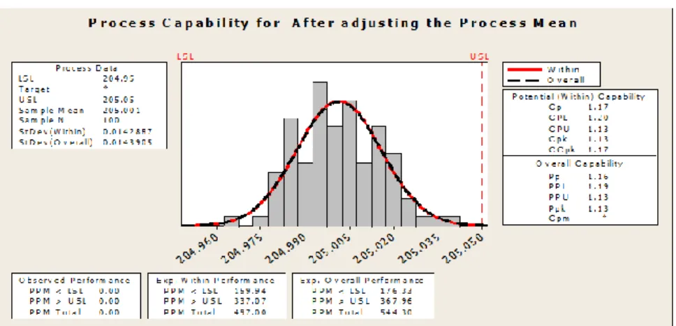
Figure 9. Process Capability Analysis before adjusting the process mean 9.2 Estimation of non-conforming Gears
(After adjusting the process Mean to specification Mean)
Figure 10. Process Capability Analysis after adjusting the process mean After adjusting the process mean, it has been
noticed that the process is under statistical control, stable over time and capable of meeting the given specification limits. Even after shifting the process mean, it has been noticed from the Figure.10, that rejections as few as 159 gears as scrap and 337 gears as rework out of 1 million gears. Still there is an opportunity to reduce the scrap and rework by identifying and reducing the
causes of variation and achieve Cp and Cpk value is 1.33.
10. Estimation of non-conforming
Gears
10.1 Estimation of confidence interval for Cp
The expressions for the above capability indices involve population parameters. In
practice, they are replaced by their sample estimations (σ‟ and ̿ ), leading to point estimates ̂ ̂ ̂ and ̂ mk .Here, confidence intervals have been provided for ̂ ̂ under the assumption of normality of the distribution of the quality characteristic. A 100 (1-α)% confidence interval for ̂ (Kushler and Hurley, 1992).
̂ √
̂ √ Where α
and α are the lower and upper α percentage points on the chi-square distribution with (n-1) degree of freedom.
√
√
,
√ √ , √ √ ,1.023 1.547 10.2 Estimation of confidence interval for
Cpk
An approximate confidence interval at 95% confidence level for Cpk has been estimated under the assumption that the quality characteristic is normally distributed. (Kushler and Hurley, 1992).
̂ √ ̂ Where n represents the sample size used to calculate ̂ and represents the standard normal value for a tail area of .
√
0.984≤ ̂ ≤ 1.33
11. Testing of Hypothesis
11.1 Testing of Hypothesis for Cp
Testing of the hypothesis has been done whether the product would be accepted by the customer, if the Cp Index for this operation exceeds 1.00, at a significance
level of 0.05.
Let, Ho: Cp ≤ 1.00, H1 = Cp >1.00 with α =
0.05
In this case, Cp=1.182. A one- sided hypothesis test with α= 0.05, at 95% lower confidence limit of Cp is obtained as below.
LCL
√
√
The hypothesized value of =1.0 < LCL. It implies that the true value of manufacturing capability Cp is not less than 1.048 with 0.95 level of confidence. Hence, the null hypothesis (Ho) can‟t be accepted and conclude that the process is capable of meeting the given specification.
11.2 Testing of Hypothesis for Cpk Testing of the hypothesis has been done whether the product would be accepted by the customer, if the Cpk Index for this operation exceeds 1.00, at a significance level of 0.05.
Let, Ho: Cpk ≤ 1.00, H1 = Cpk > 1.00 with α
= 0.05.
In this case, Cpk=1.158 .A one - sided hypothesis test with α=0.05, at a 95% lower confidence limit (LCL) of Cpk is obtained as
LCL= √
Lower Confidence Limit (LCL) =1.012 The hypothesized value of (1.0) < LCL (1.012), It implies that the true value of manufacturing capability Cpk is not less than 1.048 with 0.95 level of confidence. Hence, the null hypothesis (Ho) can be rejected and conclude that the process is capable of meeting the given specification.
12. Results and discussion
After validating the critical assumptions on the process, process capability for (before
and after adjusting the process mean) have been quantified using Cp, Cpl, Cpu , Cpk. Cpm and Cpmk indices and presented in the Table-6 , Table-5 shows commonly used capability requirement and the corresponding precision conditions. In this case, before adjusting the processes mean, Cpmk < 1.00. It implies that process was inadequate. After adjusting the process mean 1.00< Cpmk < 1.33; this indicates that the process is marginally capable and caution needs to be taken regarding the process consistency and rigid process control is required using R-Chart. After adjusting the process mean to the target value i.e., 205.00 mm, Process found to be potential as well as capable of meeting the specification and it requires close control as its Cpk value is less than 1.33. The Cp ≥ Cpm ≥ Cpmk indices show their sensitivity in exhibiting the results. The difference in the Cpmk and the Cp value indicates that the process mean is still not exactly centered with the specification limits .Table 5 shows some commonly used capability requirement and the corresponding precision conditions. Table 5. Commonly used capability requirement and the corresponding precision conditions
Precision condition Cpmk Values Inadequate
Marginally capable Satisfactory Excellent Super
Cpmk < 1.00 1.00≤Cpmk< 1.33 1.33≤Cpmk< 1.67 1.67≤Cpmk< 2.00 2.00 ≤ Cpmk
Table 6. Quantified values of Cp, Cpl, Cpu, Cpk. Cpm and Cpmk indices
Fig.no. Index
Index value before shifting the Process Mean
Index value after shifting the Process Mean
1 Cp 1.34 1.182
2 Cpk 0.026 1.158
3 Cpu 0.026 1.158
4 Cpl 2.66 1.205
5 Cpm 0.33 1.180
13. Conclusion
The case study was conducted in an automotive industry and examined using Cp,Cpk, Cpm and Cpmk index, to show the importance of process capability analysis for monitoring and ensuring the products quality to satisfy the customer‟s requirements. Before quantifying the indices, validation of the three critical assumptions were tested with the help of statistical tools like control charts, histogram and normal probability plot and run chart using the statistical software-Minitb-14.The quantified values presented in the Table 6. Shown their sensitiveness in exhibiting the results. Among all the indices
Cpmk does provide more capability assurance with respect to process yield and process loss to the customers than the other two indices Cpk and Cpm. This is a desired goal according to today‟s modern quality improvement theory, as reduction of process loss (variation from the target) is as important as increasing the process yield (meeting the specification).The construction of confidence interval for Cpk is not straight forward as that of Cp. In this paper Bissel‟s approach has been used to construct the confidence interval of Cpk, As it is significantly influenced by sample size,sample size of 100 observations is used for the process capability study.
References
:
Bissel, A.F. (1990). How Reliable Is Your Capability Index? Journal of Applied Statistics, 39, 331-340.
Carot, M.T., Sabas, A., Sanz, J.M. (2013). A new approach for measurement of the efficiency of Cpm and Cpmk control charts, International Journal for Quality Research, 7(4), 605-622. Chen, K.S., Pearn,W.L., Lin, P.C. (2003). Capabilit measures for processes with multiple
characteristics, Quality and Reliability Engineering International, 19, 101-110.
Gildeh, B.S., & Asghari, S. (2011). A new method for constructing confidence interval for Cpm based Fuzzy data, International Journal for Quality Research, 5(2), 67-73.
Gunter, B.H. (1989). The use and abuse of Cpk ,1-4, Quality Progress, 22(1), 72-73(3), 108-109(5), 79-80(7).
Juran, J., Gryna, F., (1988). Juran's Quality Control Handbook, 4th edition., McGraw-Hill ,New York.
Kumar, S.G., (2010). A quantitative approach for detection of unstable Processes using a run chart. Quality Technology and Quantitative Management, 7(3), 231-247.
Kushler, R.H. (1992). Confidence Bounds for Capability Indices. Journal of Quality Technology, 24(4), 118-195.
Montgomery, D.C. (2000). Introduction to Statistical Quality Control, Fourth Edition, John Wiley and Sons, Inc.
Prabhuswamy, M.S., & Nagesh, P. (2007). Process capability Analysis made simple through graphical approach, Kathmandu University. Journal of science, Engineering and Technology, 1(3).
Prabhuswamy, M.S., Nagesh, P. (2010-2011). Process capability validation and short - Long term process Capability Analysis with case study, Proceedings of ETIMES-2006.
Ray, S., & Das, P. (2011). Improving machining process capability by using Six Sigma,
Yerriswamy Wooluru JSS Academy of Technical Education,
Bangalore-560060 India
Swamy D.R
JSS Academy of Technical Education,
Bangalore-560060 India
P. Nagesh
Sri Jayachamarajendra College of Engineering, JSS Centre for Management studies
Mysore-570006 India