Electrical Engineering Vol. 16, No. 1, pp. 19{33
c
Sharif University of Technology, June 2009
Practical Next Bit Test for
Evaluating Pseudorandom Sequences
A. Lavasani
1and T. Eghlidos
2;Abstract. The Next Bit Test briey states that a sequence is random if and only if, given any i bits of the sequence, it is not possible to predict the next bit of the sequence with a probability of success signicantly greater than 1=2. In 1996, Sadeghiyan and Mohajeri proposed a so-called \new universal test for bit strings", based on the theoretical next bit test. In this paper, we study dierent aspects of this test and show its weakness. Then, we improve it both theoretically and practically for better classication of the sequences. As a result, a Practical Next Bit (PNB) test is introduced in two Global and Local versions and a histogram, which gives an impression of the global evaluation of the underlying sequence. Testing samples of nonrandom sequences, using both the PNB test and the NIST Statistical Test Suite, indicates the superiority of the PNB test power over that of the NIST.
Keywords: Next bit test; Random sequences; Statistical test.
INTRODUCTION
Random (or pseudorandom) sequences play an essen-tial role in many elds. When there is a need to model a dynamic system or in the implementation of a simulation program, the use of random sequences is inevitable. However, in cryptographic applications, considering the sensitivity of the information, ran-domness is the major concern [1]. The output of an encryption algorithm is required to be random as a necessary condition of security. Cryptosystems do not reach their security level unless random keys are employed. Many cryptographic protocols, like digital signatures and challenge-response schemes, use random sequences as auxiliary quantities.
In regard to the above mentioned facts, distin-guishing random from nonrandom sequences is critical in scientic areas and should be treated even more strictly in cryptology. Since the introduction of modern ciphers, various statistical tests have been developed, each of which assessing the presence or absence of
1. Department of Mathematics, Sharif University of Technology, Tehran, P.O. Box 11155-8639, Iran.
2. Electronics Research Center, Sharif University of Technology, Tehran, P.O. Box 11155-8639, Iran.
*. Corresponding author. E-mail: [email protected] Received 18 August 2007; received in revised form 20 August 2008; accepted 11 October 2008
a \Pattern" in the output of the ciphers. Such a pattern, if detected, would indicate that the sequence is nonrandom [2]. In searching for a criterion to test randomness, in 1982 Blum and Micali [3] were the rst to show that the ability of predicting the next bit of a sequence is enough to judge the sequence to be nonrandom. Yao [4] formalized the idea in [3] by stating that a sequence is random if and only if every probabilistic polynomial-time algorithm fails to predict the next bit of the sequence with a signicant probability.
However, using the universal quantier (every algorithm) in Yao's statement connes it to a merely theoretical rather than practical test. There has been some eort to deduce practical tests based on this theoretical idea. As a typical example see [5]. Another test algorithm was designed by Sadeghiyan and Mohajeri, called the \new universal test for bit strings", which presents a practical test for pseudo-randomness, based theoretically on an extension of Schrift and Shamir's next bit test [6], in order to realize the theoretical universal next bit test at least partially [7]. Throughout this paper, we re-fer to this test as the Sadeghiyan-Mohajeri test. However, the Sadeghiyan-Mohajeri test did not ap-pear to be a powerful randomness test becouse of some holes in the test algorithm. In this paper, the authors show that this test cannot distinguish
between pseudorandom and highly nonrandom se-quences.
In this work, the Sadeghiyan-Mohajeri test is improved in both theoretical and practical aspects and extended to provide a deeper analysis of randomness. By introducing the Extended Next Bit test, the the-oretical problem of the test is solved. Then, the algorithm is improved by modifying some of its steps. By applying these improvements to the test, we call it the Practical Next Bit (PNB) test.
The authors assess the performance of the PNB test and show that it can remedy the disability of the original proposed test. Then, it is compared with other tests, which have been standardized by the National Institute of Standards and Technology (NIST) [2]. Practically, the performance of the PNB test is shown. Although it consumes more time and memory for many sample sequences it shows more precise results compared with several NIST tests, in the sense of nding randomness anomalies in the sequence. The complexity of the test is not regarded as a problem anymore because the new technology provides users with faster processing and a greater amount of memory. The authors believe that accompanying the PNB test with the NIST statistical test suite sig-nicantly increases the power of cryptanalysts in detecting nonrandom behavior in cryptographic se-quences.
The outline of this paper is as follows: First, the notations and denitions used throughout this paper are briey introduced, and then an introduction to the Sadeghiyan-Mohajeri test and the Practical Next Bit test are given. Following that, the theoretical base of the PNB test is redened and the authors give a theoretical improvement of the Sadeghiyan-Mohajeri test from a global point of view. The following section is devoted to the PNB test and the corresponding algorithm. The benchmarks for comparing the global test with the NIST's along with the experimental results bring this section to an end. Then, the theoretical aspect of predicting more than one bit is discussed, which results in introducing the local PNB test. After that, the algorithm for obtaining the histogram from a sequence is given. Finally, all discussions and results giving an overall view on this paper along with concluding remarks are presented.
PRELIMINARIES
Denitions and Notations
In this section, some notations and denitions used frequently throughout this paper are briey introduced. These notations are the same ones used by Schrift and Shamir [6]. Let sn
1 denote a binary sequence of length
n in f0; 1gn. The ith bit of the sequence is denoted
by si, while a subsequence starting with the jth bit
and ending with the kth bit (1 j < k n) is denoted by sk
j. The notation O((n)) is used for any
function, f(n), that vanishes faster than the inverse of any polynomial, that is for every polynomial, poly (n), and n large enough, f(n) < 1=poly (n). Also, in the context of the test denition, notation A is used to denote every probabilistic polynomial time algorithm, A : f0; 1gi 1 ! f0; 1; g. Throughout this paper, the
leftmost bit is considered the least signicant, since the sequence length is unknown.
Denition 1 [7]
A binary source, S, passes the next bit test if, for every i; 1 < i n and every probabilistic polynomial-time algorithm, A: f0; 1gi 1 ! f0; 1g, the following
inequality holds: probSfA(si 1
1 ) = sig 1=2 O((n)): (1)
SADEGHIYAN-MOHAJERI TEST Motivation
In order to evaluate a sequence from the view of randomness, there exist several statistical tests, which compare the overall behavior of the sequence with some particular probabilistic models.
A statistical test that measures the randomness of a sequence was presented by Sadeghiyan and Mo-hajeri [7]. This test was designed, based on the pre-dictability of the next bit of the underlying sequence, given the former bits. In this section, the theoretical base of this test and the detailed description of the algorithm are presented.
Theoretical Base of Sadeghiyan-Mohajeri Universal Test
The Sadeghiyan-Mohajeri Universal Test was pre-sented, based on the ideas of statistical tests and the Predict Or Pass (POP) Test of Schrift and Shamir [6] presented in Denition 2. Based on their proposed test, Sadeghiyan and Mohajeri claimed that the Universal Test attempts to implement the concept of Yao's theoretical Next Bit test [7].
Denition 2 [7]
A biased source, S, with a xed bias, b, 1=2 b < 1, passes the Extended-POP test, if for every i and l, 1 < i, l n, for every xed c and every probabilistic polynomial time algorithm:
A: f0; 1gi 1! ff0; 1gl; g;
if prob fA(si 1
1 ) 6= g 1=nc;
then probSfA(si 1
1 ) = si 1+li jA(si 11 ) 6= g b
O((n)): (2)
The Sadeghiyan-Mohajeri Test
In this part, we introduce the Sadeghiyan-Mohajeri test. The test algorithm takes advantage of a tree structure, which stores information on the patterns or subsequences in the sequence.
The counting of m-bit patterns can be depicted as a weighted tree, which is called a pattern tree. In
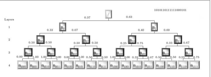
the pattern tree, each node in depth l represents the number of occurrences of a binary pattern of length l in the underlying sequence. In this weighted tree, each edge connecting two nodes denotes the ratio of the number of child patterns located in the next layer to the number of their parent patterns in the previous layer [7]. As an example, a 16-bit sequence and the related pattern tree is depicted in Figure 1. According to the above explanation, the number of each pattern can be computed by adding the numbers associated with its child patterns. For a large enough random sequence, it is expected that all the ratios corresponding to the edges of the pattern tree to be approximately equal to 1=2.
Algorithm 1 presents the Sadeghiyan-Mohajeri test [7] for sequence of length, n.
Figure 1. Pattern tree for the rst 16 bits of binary expansion of e, the conditional probability of the occurrence of each pattern (node) on each branch given the parent pattern.
The Sadeghiyan-Mohajeri test does not give any precise explicit criteria for global judgment about the randomness of the sequence. Instead, the designers suggested deriving a histogram for each sequence, which can give a general idea about its global random behavior. When the algorithm successfully predicts a block of (l + 1) bits after a pattern, it admits that a local non-randomness has occurred in the sequence. REDEFINING THE THEORETICAL BASE OF THE PNB TEST
The method of choosing decision threshold in the Sadeghiyan-Mohajeri test shows that the probabilistic algorithm predicts when the next bit of a block occurs with a probability signicantly dierent from 1=2. Therefore, with an appropriate choice of signicance level, the sequence generated from a non-uniform random generator fails in this test. However, the Extended-POP test accepts such biased sequences as random ones independent of any signicance level. Therefore, it cannot be a basis for the Mohajeri test. So, we can state that the Sadeghiyan-Mohajeri test works, based on the Extended Next Bit (ENB) test, which we present in the next part. In fact, this test is a natural extension of the next bit test and provides a theoretical basis for the Sadeghiyan-Mohajeri test.
Extended Next Bit Test Denition 3
A binary sequence, sn
1, originated from source S, passes
the ENB test if for every i and l, 1 < i, l n, and for every probabilistic polynomial time algorithm, A: f0; 1gi 1! f0; 1gl, such that either A(si 1
1 ) = means
A cannot predict the next bit(s), or if A predicts the next bit(s), then the following inequality holds:
probSfA(si 11 ) = si 1+li g (1=2)l O((n)): (3)
Theorem 1
The following statements are equivalent: i) The Next Bit test,
ii) The Extended Next Bit test. Proof: See Appendix A.
Hence, we can consider the Sadeghiyan-Mohajeri test as an algorithm for the ENB test, and NOT an algorithm for their proposed Extended-POP test, since the non-uniform (biased) pseudorandom sequences fail the Sadeghiyan-Mohajeri test theoretically.
IMPROVING THE
SADEGHIYAN-MOHAJERI TEST FROM THE GLOBAL VIEW
The Relation Between Theoretical and Practical Next Bit Tests
As mentioned in Denition 3, the next bit test dis-qualies a supposedly random sequence whenever there exists a polynomial-time algorithm that can predict the next bit of that sequence, given all its previous bits. Any polynomial-time algorithm, which can predict the next bit (or equivalently some next bits) of a sequence, is a disqualier of that sequence. Regarding the ran-domness denition [3], it can be proven mathematically that such a sequence is globally nonrandom. In this sense, the PNB test is an instance of such a polynomial-time algorithm.
Our next step is to improve the performance of the test algorithm.
The Depth of Start Layer
The Sadeghiyan-Mohajeri test assumes that each sub-sequence of a certain length of underlying sub-sequence is known to the algorithm. In the next step, the algorithm tries to predict the next bit of those subsequences and uses the result of this step to judge about the randomness of the complete sequence. Ideally, all previous bits of the complete sequence are known to the algorithm to predict its next bit. However, as the prediction process relies on the statistics deduced from the sequence itself, the society of the bits of the sequence is too small to be regarded as a reference for inferring any information about the next bit of the whole sequence. Instead, we can exploit information about the distribution of the next bit of relatively short subsequences of the original sequence, using that society.
In this section, we try to nd out which length of subsequences best suits this purpose.
The Relation Between Next Bit Prediction and the Depth of Start Layer
In the rst step of Algorithm 1, for each pattern in the pattern tree, the algorithm checks if the number of occurrences of the child of a specic pattern ending with 0 diers signicantly from that ending with 1; the algorithm predicts the next bit of the subsequence.
As depicted in Figure 1, the depth of each layer of the tree is equal to the length of the patterns (that is corresponding subsequences in the underlying sequence) of that layer. According to the above-mentioned structure we dene the Depth of Start Layer as follows.
The pattern for which the algorithm compares the number of occurrences of its children, is called
the Known Pattern; the layer in the pattern tree including all known patterns (which belong to the same layer) of the tree is called the start layer. The length of those patterns remains constant during each run of the algorithm, and is equal to the depth of the corresponding layer in the pattern tree. This length is called the Depth of Start Layer.
Algorithm 1 sets the depth of start layer equal to l = log2(n) 1. This length was chosen, since it is possible for a sequence of length n to contain all possible subsequences of length l + 1 [7].
However, as the prediction process is independent of choosing the depth of the start layer, it is possible to choose a better depth for the start layer other than l.
The prediction process does nothing other than running a frequency test [2] on the bits occurred after each subsequence. Then, it computes the 2 statistic
of this observation and uses it to test if the observation can signicantly result in the rejection of the null hypothesis, which states that the next bit(s) of the underlying subsequence have a Bernoulli distribution with a mean of 1=2. However, the 2 test is not
applicable to all random experiments. Knuth [8] stated that the 2 distribution is an approximation that is
valid only for a large enough number of observed experiments. Accordingly, if we repeat a random experiment k times, a common rule of thumb is to take a large enough k, such that each of the expected values occurs ve or more times, otherwise the test is not valid and we cannot rely on its result [8]. In our case, where the random sequence bits have an independent Bernoulli distribution with a mean of 1=2, we need the subsequence to be repeated k = 2 5 = 10 times along the sequence to fulll the validity criterion of the 2
test.
Algorithm 1 does not consider the validity of the 2 test; it leads to some unreasonable prediction and
disqualies some pseudorandom sequences.
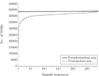
To quantify the above statement, we dene the notion of occurrence of nonrandom behavior. Suppose that a pattern fails the test and, consequently, it is possible for the prediction algorithm to predict its next bit. Any occurrence of such patterns in the pattern tree of the underlying sequence is called an Occurrence of Nonrandom Behavior (ONB).
Figure 2 gives evidence of the weakness of the Sadeghiyan-Mohajeri test. The pseudorandom se-quences are generated by the double AES encryption of the output of SHA-2. Both algorithms are believed to show good randomness properties in their output [9,10]. On the other hand, the nonrandom sequences are either extracted from graphical data or compression of texts and executable programs. As can easily be seen, the Sadeghiyan-Mohajeri test nds more ONBs in sequences from a pseudorandom category than those from nonrandom ones.
Figure 2. Comparison between the number of ONBs resulting from executing Sadeghiyan-Mohajeri test on pseudorandom and nonrandom categories.
In fact, a subsequence with length l = log2(n) 1 is too large to happen 10 times in an n-bit sequence. More precisely, the expected number of times that such a subsequence occurs in an n-bit random sequence can be calculated as follows:
(The total no. of overlapping patterns that can be tted into the reference sequence) (The no. of possible patterns with length l)
= 2nl = 2: (4)
It means that we do not expect to be able to apply the 2 test for any pattern length and the test might
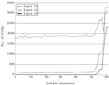
have no result for many sequences with no obvious non-random behavoir. However, using l = log2(n) 2 as the depth of the start layer, the clear deviation from randomness is still detectable. The practical results, depicted in Figure 3, signify the same fact.
From the other aspect, the way of prediction of the next bit of subsequences within a sequence can be related to the reference sequence, using binomial distribution.
Each subsequence of length equal to the depth of the start layer can be considered an occurrence of either random or nonrandom behavior. Therefore, the state of all such subsequences, with the length equal to the depth of the start layer, is a random variable with binomial distribution. It is always desirable to approximate binomial distribution with the normal distribution because it makes the computation easier. However, this approximation is only valid when the mean of the binomial distribution is greater than 10 [11]. In this context, by \mean of the binomial distribution", we mean the average number of ONBs corresponding to a random sequence. It is not easy to calculate this average number by sticking only to the
Figure 3. Comparison of the number of occurrences of nonrandom behavior w.r.t. the sample sequences computed for three dierent start layers.
theory; nevertheless we can obtain it by the practical results of the test on pseudorandom sequences. Using normal distribution as an approximation to the bino-mial distribution leads us to choose the depth of the start layer, which provides us with an average number of ONBs more than 10.
Practical Results of the Dierent Layers In order to nd the suitable layer to be taken as the start layer, the PNB test was run on the 61 sample sequences shown in Table B1, Appendix B, for start layers with depth 1 to 24 (where no nonrandom behavior is detected). The result of layers 14 to 16 is depicted in Figure 3.
Setting start layer one from the rst to the 14th, we observe that the curve does not show any signicant dierence between the number of ONBs of pseudorandom (the sequences in the rst and the second categories, according to Table B1) and that of nonrandom sequences (third category). How-ever, there are intrinsic dierences in their generation methods, which NIST tests can signicantly distin-guish.
Regarding the 16th to 24th layers as start layers, the dierence between pseudorandom and nonrandom sequences can easily be observed. However, the number of ONBs in pseudorandom sequences is too small to be a basis for comparing the randomness quality of pseudorandom sequences with each other.
Among these layers, the result of the 15th layer is an acceptable distinguisher between pseudorandom and nonrandom sequences and, on the other hand, the wide range of 80 to 140 ONBs (the dierence between the ONB of the rst and the 52nd sample sequences in Figure 3) provides a good tool for ranking the quality of pseudorandom sequences, compared with those of the 16th layer.
Moreover, by choosing the 16th layer as the start layer (as is considered in the original design of the Sadeghiyan-Mohajeri test) the average number of ONBs in a pseudorandom sequence becomes 2.8 for the experimental sample. As stated previously, a binomial distribution with such a \mean" cannot be approximated by a normal distribution. The mean of 103.2 of the 15th layer, however, fulls the prerequisite of the approximation.
Improved Depth of the Start Layer
Considering both the theoretical and practical results, it seems that log2(n) 2 is a more proper choice for the start layer than log2(n) 1, which is proposed
in Algorithm 1. The reasons are as follows: First, the variety of the patterns in the (log2(n) 1)th layer results in their less frequent occurrence in the sequence, which causes the 2 validity condition to be
rarely satised; for most patterns, their randomness cannot be judged. Second, the average number of ONBs in this layer is too small to approach the normal distribution. Finally, the inability of this layer in ranking pseudorandom sequences weakens the power of this test in discovering nonrandom sequences with higher levels of entropy (Figure 3).
Study of the Length of Prediction Block Length of Prediction Block in the
Sadeghiyan-Mohajeri Algorithm
In [7], the authors suggested that a node is recognized as an ONB if more than l bits can be predicted after it. Moreover, it is claimed that in such a situation there is a block of length l, where its next block could be guessed and the sequence may be rejected as being generated with a random generator under the required properties.
This criterion is more heuristic than mathe-matical, and for nding a prediction length upon a mathematical basis, we should observe the process of predicting subsequent bits. According to Algorithm 1, for each pattern in the (l 1)th layer, when the algorithm predicts its lth bit, it omits the left most bit of the resulted l bit pattern to achieve another (l 1)-bit pattern, which again is a node of the start layer. Again, if this new pattern is an ONB, its next bit, that is the (l + 1)th bit of the original pattern, is predictable. The algorithm stops when either it meets a pattern whose next bit is unpredictable or it loops these steps l + 1 times. In the latter case, it admits that the original pattern is an ONB.
Assessing and Improving the Original Length of the Prediction Block
For studying the proper length of the prediction block, we employ the discrete random variable, Xi, which
shows the nonrandom behavior in the ith pattern of the lth layer of the tree such that:
Xi= 0, if the next block after the ith pattern is
not predictable.
Xi= 1, if the next block after the ith pattern is
predictable.
By this convention, the number of ONBs in the underlying sequence is a random variable, Y , as follows:
Y =X2l 1
1 Xi: (5)
If we set the length of the prediction block equal to 1 (that is we only predict one bit to admit an ONB), the Xi variables are independent of each other.
Under this condition, according to the number of patterns in the (l 1)th layer (in the way that we have chosen previously) and the fact that all Xis are
identically distributed, the Central Limit Theorem can be employed to deduce that Y is normally distributed. Knowing the probability distribution of Y enables us to nd easily the P -value for this test.
However, if we admit an ONB whenever it is possible to predict more than one bit, the Xi variables
are not independent any more. Actually, predicting the second bit of a pattern is the same as the prediction of the rst bit of the next pattern shifted by one bit. In this case, due to the lack of independence between Xis,
we cannot approximate the distribution of Y as normal, using the central limit theorem.
A deeper look at the Sadeghiyan-Mohajeri test reveals that the number of patterns, whose one next bit is predictable, is an estimation of the number of patterns, whose k next bits are predictable.
Improved Length of the Prediction Block According to Theorem 1, there is no theoretical dif-ference between predicting one or more bits. For this reason, and also because of the results of this section, we exploit the advantages of predicting one next bit of a pattern within a given sequence as a sign of ONB. Hence, in our proposed randomness test, we set the length of the prediction block equal to 1.
The Improved Test
By applying the improvements of this section to the Sadeghiyan-Mohajeri test, we introduce the PNB Test in the next section.
THE PNB TEST The Algorithm Test Purpose
The purpose of this test is to determine whether there is a deviation in the statistic of the next bits of a
subsequence whenever it appears; if there is such a deviation, then the test exploits it to predict the next bit of the subsequence. A sequence is considered nonrandom if it contains many subsequences whose next bit is predictable.
Test Statistic
Let Yobs be the number of ONBs in the pattern
tree of the sequence, that is equal to the number of subsequences whose next bit is predictable.
The reference distribution for this test statistic is the normal distribution (see previous sections). Test Description
Note that since no known theory is available to de-termine the exact values of and for the last step of Algorithm 2, these values were computed (under the assumption of randomness) using a double AES encryption of SHA-2 with dierent random keys for each session [2]. Refer to Appendix B for further details.
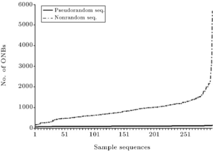
As expected, the PNB test shows more reason-able results in comparison to the original Sadeghiyan-Mohajeri test. The PNB Test can easily distinguish between pseudorandom and nonrandom categories of sequences, as depicted in Figure 4.
Global Test Versus NIST's
The Benchmarks for Comparing the Global Test with the NIST's
NIST proposed a Statistical Test Suite [2], which is a package consisting of 16 tests. These were developed to test the randomness properties of binary sequences. These tests focus on a variety of dierent types of non-randomness that could exist in a sequence. Although it is not claimed that this suite can completely assess all aspects of randomness of the underlying sequence,
Figure 4. Comparison between the number of ONBs resulting from executing the PNB test on pseudorandom and nonrandom categories.
Algorithm 2. Practical next bit test. they are considered as being useful in detecting its
deviations from randomness [2].
As a measure of qualication, we compare the power of the PNB test with that of NIST's.
Denition 4
The power of a statistical test is the probability that the test will reject a false null hypothesis, or in other words, it will not make a Type II error [12].
In this context, the power of a test is the probabil-ity that the underlying test will not admit a nonrandom sequence as being random. As power increases, the chances of a Type II error decrease and vice versa.
Having higher power makes for a more ecient test; eciency in the sense that the user can have condence in the random behavior of a generator by testing a smaller sample. Also, the nonrandom behavior of a bad generator can be discovered by testing a smaller number of outputted sequences.
One of the primary goals of introducing the NIST test suit was to minimize the probability of a Type II error [2]; it is reasonable to employ the new test, which makes this kind of error less probable. However, it does
not mean that other tests can be replaced by the PNB test, as the new test merely checks a new aspect of randomness, but it does not cover the aspects checked by the other tests.
Both the PNB and the NIST tests are run on three categories of nonrandom sample sequences in Appendix B. NIST tests are executed using the NIST recommended parameters. For each category, the tests are ranked according to the power they showed corre-sponding to that category. The results are depicted in Tables C1 to C3, Appendix C.
Experimental Results
Tables C1 to C3 in Appendix C show a comparison between the power of the PNB test and NIST's. In all the three categories, the PNB test is privileged in recognizing nonrandomness within the sequence, as its power ranked rst in all the three categories. In other words, there are some nonrandom anomalies in the sequences, which remain undetectable considering the NIST tests.
The PNB test judges the global random behavior of a sequence by nding the local nonrandom
occur-rences that happen in the sequence. The judgment is based on the assumption that the diversity of the patterns in the sequence is as high as the expected value for a random sequence. To fulll this assumption, it is crucial that a pattern diversity evaluator test is executed. A practical suitable example of such a test is the serial test [2]. In other words, the PNB test makes sure that the occurrences of existing patterns in the sequence are independent of each other, but it does not judge about their mere existence. The result of the PNB test cannot be considered valid on a sequence that fails the serial test.
It is also worth mentioning that the experimental computation of the test distribution shows that the PNB test is not conservative.
IMPROVING THE
SADEGHIYAN-MOHAJERI TEST FROM THE LOCAL POINT OF VIEW
Sadeghiyan-Mohajeri's Algorithm for Prediction of More Than One Bit
In this part, we want to study, in more detail, the way that Algorithm 1 predicts each bit of the next block. Study of Sadeghiyan-Mohajeri's Algorithm for the Next Block Prediction
Theoretical View
Although the prediction process of Algorithm 1 does well in predicting the rst bit of the predicted block, the algorithm seems not to be valid for predicting more than one bit. Our deduction about the second next bit of an (l 1)-bit pattern could be inuenced by another l-bit pattern that has the same bits as the derived l-bit pattern (the concatenation of the (l 1)-bit subsequence with the predicted 1)-bit) except for its leftmost bit, which diers from the leftmost bit of the (l 1)-bit subsequence. The statistics of such a pattern interfere in the prediction process and leads us to a wrong result. The following lemma states this claim mathematically.
Lemma 1 Let sl 1
1 be the primary pattern and the algorithm
predict its second next bit, a 2 f0; 1g. Then, the following assertion holds:
prob(sl+1=ajsl1)6=prob(sl+1=ajs2l; s1)prob(s1jsl2)
+ prob(sl+1= ajsl2; s1)prob(s1jsl2): (6)
Proof: The left hand side of Relation 6 is the de-nition of predicting the next bit, given the previous l bits. However, the local nonrandomness detector algorithm computes the right hand side and outputs
the wrong result, because the second term at the right hand side of Relation 6, namely prob(sl+1 =
ajsl
2; s1)prob(s1jsl2), is totally unrelated to the second
next bit of the underlying pattern. It is, however, considered in the prediction process and dismisses its validity.
Practical View
To evaluate the Sadeghiyan-Mohajeri's prediction pro-cess, the Sadeghiyan-Mohajeri test has been carried out on a sample of random sequences to predict two bits of each subsequence. The number of bits that have been predicted wrongly has been signicantly higher than the theoretical expectation. This rejects the validity of the sequential prediction algorithm in practice as well.
Correction of the Sadeghiyan-Mohajeri's Algorithm
The main problem with the sequential prediction in the next block method is that it does not include the known information in the prediction process. For example, the leftmost bit of the original subsequence is known. However, it is not used in the prediction of the second and further next bits of that subsequence. We solve this problem as follows.
Let the prediction of k bits after a pattern indicates the local nonrandomness behavior of the underlying sequence, whenever such a pattern exists. The tree constructed for this algorithm is no longer a binary tree. Instead, a B-Tree [12] of 2k children
(that is the number of all possible patterns of k-bit length) for each node is constructed. Note that k is a xed value, which should not depend on the length of the sequence, otherwise, the algorithm would no longer be polynomial time. For each child of each pattern, the algorithm counts the number of occurrences of that child after the subsequence in the underlying sequence. Then it judges the ran-domness of the pattern by performing a goodness-of-t test for the equal occurrence of its children. If the pattern fails the test, the local nonrandom behavior is reported, wherever that pattern occurs in the sequence.
As long as the 2 test is valid, the choice of
greater k results in a greater number of nonrandom patterns. Therefore, regarding the sensitivity of the case, users can specify the desired length of the pre-diction block. The validity condition of the 2 test,
as stated previously, requires that the length of the parent pattern (depth of start layer) should be short enough to permit the occurrence of total 2k 5 times
of each subsequence (parent pattern) in the sequence. The probability of the validity condition of 2decreases
chosen. From the point of view of complexity, there is a trade-o between the length of the prediction block and the memory needed to store the B-Tree of 2k children. In other words, increasing the length
of the prediction block causes the memory needed for storing the B-Tree to grow exponentially making execution of the test much harder or even impossible. Therefore, users should wisely choose a short prediction block to get valid practical results. By applying this solution, we present the local PNB test in the next section.
LOCAL TEST Algorithm Test Purpose
The focus of the local next bit test is on nding the subsequences in the sequence for which some of the next bits are predictable.
The Test Statistic and Reference Distribution Let i
obs be a measure, for each possible ith
sub-sequence of length l, which indicates how well the observed proportion of the next l0 bits after that
subsequence match the expected proportion, 1 2l0.
The Test Description
A description of the local test is given in Algorithm 3.
NEXT BIT HISTOGRAM
In order to have evidence of the randomness behavior of a sequence, it is desirable to have a histogram which plots an intuitive scheme of the nonrandom behavior of that sequence.
Construction
The histogram of the practical next bit test uses the same idea as the Sadeghiyan-Mohajeri's histogram [7]. Therefore, the new histogram is constructed by the same method, but supports more exibility. The histogram construction algorithm runs several local tests, setting dierent lengths for the prediction block. Each node of the histogram shows the number of local nonrandomness with a specied length of prediction. Algorithm 4 shows the detailed process of the his-togram construction.
Interpretation of the Results
Many heuristic results can be obtained by looking at the PNB histogram. Here, we just point out the obvious ones.
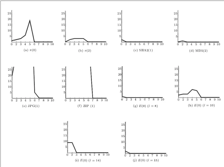
As can be observed from Appendix D, Figures D1, most of the histograms start with a positive slope, reach a peak and then decrease. The less the area covered by the histogram, the more the random properties of the tested sequence. Naturally, the histogram should increase and decrease steadily. If in a sequence the
Algorithm 4. Practical Next Bit test histogram. histogram becomes at after it passes the peak, a
serious local nonrandomness is expected to occur in some subsequences of the sequence.
CONCLUSIONS
In this paper, the Sadeghiyan-Mohajeri test was stud-ied and analyzed from both theoretical and practical aspects. First, contrary to the authors' claim, it was proved that the Sadeghiyan-Mohajeri test does not rely on the proposed Extended-POP test as a theoretical basis. Instead, the Extended Next Bit (ENB) test was introduced as the theoretical basis for the Sadeghiyan-Mohajeri test and proved to be the equivalence of the Next Bit test and ENB test. Then, the authors derived the Practical Next Bit (PNB) test from the Sadeghiyan-Mohajeri test in two new versions; Global Next Bit test and Local Next Bit test.
For the Global version, dierent aspects of the Sadeghiyan-Mohajeri test were studied to improve its power in recognizing nonrandom behaviors in the underlying sequence. Then, the length of the prediction block was replaced from the proposed log2(n)+1 bits to one bit and the validity condition of the goodness-of-t test was considered during the prediction. Using both theoretical and practical results, the authors chose the (log2(n) 2)th layer as the best start layer. By applying these improvements, it was called the PNB test and signicant improvements in its results were observed.
In the next step, we suggest a way to compute the P -value corresponding to every applied sequence.
The standardization makes it possible to compare the PNB test with the existing tests such as NIST's. Experimentally, the superiority of the PNB test in nding nonrandomness anomalies was shown.
To solve the problem in the Sadeghiyan-Mohajeri test algorithm, while predicting more than one bit, the authors have introduced a new algorithm for the Local Next Bit test. Using this algorithm for predicting more than one bit, a new histogram has been introduced, which can give the user a better impression, view and comparison tool for the global random behavior of the underlying sequence.
Considering the experimental results of the power comparison and the variety of the information about the randomness of the sequence (the global randomness behavior via P -value calculation, drawing a histogram and the local nonrandomness behavior), the authors suggest that the user runs the PNB test prior to the other tests, among them the NIST tests, for analyzing the random behavior of the underlying sequence.
Moreover, the Local Next Bit test enables the user to nd the exact positions of nonrandom behavior in those sequences used for cryptographic applications.
Obviously, one cannot claim that there exists an optimal statistical test which can detect all nonrandom behaviors of every sequence. This is also true for the PNB test. Certainly, further research in this eld will result in more ecient test algorithms.
ACKNOWLEDGMENTS
Our sincere thanks go to Dr. Babak Sadeghiyan whose guidance was crucial to the complete understanding of the original test. We also thank Prof. Yogendra P. Chaubey for his valuable advice in acquiring ex-perimental results. Finally, we thank the Research Vice-Presidency of the Sharif University of Technology, whose nancial support enabled us to accomplish this research work.
REFERENCES
1. Junod, P. \Cryptographic secure pseudo-random bits generation: The Blum-Blum-Shub generator", http://crypto.junod.info/bbs.pdf (Aug. 1999). 2. Rukhin, A. et al. \A statistical test suite for
ran-dom and pseudoranran-dom number generators for crypto-graphic applications", NIST Special Publication 800-22, http://csrc.nist.gov/publications/ nistpubs/800-22/sp-800-22-051501.pdf (2001).
3. Blum, M. and Micali, S. \How to generate crypto-graphically strong sequences of pseudo-random bits", [FOCS] 1982; SIAM J. on Computing, 13(4), pp. 850-864 (1984).
4. Yao, A.C. \Theory and applications of trapdoor func-tions", Proc. 23rd IEEE Symp. on Foundations of Computer Science (FOCS), pp. 80-91 (1982).
5. Hernandez, J.C., Sierra, J.M., Mex-Perera, C., Borrajo, D., Ribagorda, A. and Isasi, P. \Using the general next bit predictor like an evaluation criteria", Proc. NESSIE workshop, Leuven (Belgium), http://www.cosic.esat.kuleuven.be/nessie/workshop/ (Nov. 2000).
6. Schrift, A.W. and Shamir, A. \Universal tests for non-uniform distributions", Journal of Cryptology, 6, pp. 119-133 (1993).
7. Sadeghiyan, B. and Mohajeri, J., A New Universal Test for Bit Strings, ACISP'96 LNCS Series, Springer Verlag, pp. 311-319 (1996).
8. Knuth, D., The Art of Computer Programming, 2, Addison-Wesley (1993).
9. FIPS-197, National Institute of Standards and Technology \Advanced encryption standard", http://csrc.nist.gov/publications/ps/ps197/ps-197.pdf (Nov. 2001).
10. FIPS 180-2, National Institute of Standards and Technology \Secure Hash Standard (SHS)", http://csrc.nist.gov/publications/ps/ps180-2/ps180-2withchangenotice.pdf. (Aug. 2002). 11. Ghahramani, S., Fundamentals of Probability, 2nd Ed.,
Prentice-Hall, New York, USA (2000).
12. Cohen, J., Statistical Power Analysis for the Behav-ioral Sciences, 2nd Ed., Lawrence Erlbaum, Asso-ciates, New Jersey, USA (1988).
APPENDIX A Proof of Theorem 1
The following statements are equivalent: i) The Next Bit test,
ii) The Extended Next Bit test.
Proof: First we prove that (i) ! (ii) or, equivalently, : (ii) ! : (i).
If the underlying sequence fails in the ENB test, then there exists i, l and a probabilistic polynomial time Algorithm A, such that it can predict the next l bits of si 1
1 with probability p, that is:
jp (1=2)lj O((n)): (A1)
Let r be the l bit output sequence of A, then there exists some j; 0 j l 1, such that:
jprobSfrj+1= si+jg 1=2j O((n));
otherwise, we face a contradiction to Relation A1. Therefore, the following inequality holds:
jprobSfA(si+j 11 = si+jg 1=2j O((n)): (A2)
Relation A2 reveals that the underlying sequence fails in the Next Bit (NB) test. Now, we prove that (ii) ! (i).
If the underlying sequence passes the ENB test, then it passes the test for every l; 1 l n.
So, by setting l = 1, the sequence also passes the NB test.
APPENDIX B Sample Sequences
Sample Sequences for Finding Suitable Start Layer
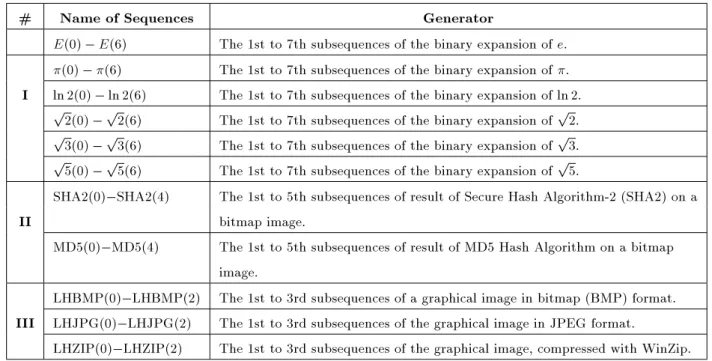
The chosen spectrum, from pseudorandom to highly nonrandom sequences, is used for experimental tests to nd a proper start layer. These sequences are listed in Table B1. All of the sequences have the same length of 128 Kbits, but they are categorized in three sections: Binary expansion sequences of some irrational numbers, the sequences resulted from standard hash algorithms and ordinary data sequences resulted from some graphical data. The rst and second ones are assumed to be pseudorandom, but the third one contains highly nonrandom data.
Sample Nonrandom Sequences for Comparison Between Dierent Tests
The three categories of nonrandom sequences are used for the comparison purpose. These sequences are listed in Table B2. All of the sequences have the same length of 128 Kbits, but they are categorized in three sections, that is sequences resulted from lossy compression of graphical data in frequency space (JPEG), sequences resulted from lossless compression of graphical images with the LZW algorithm (GIF) and sequences resulted from compression of executable programs and texts using the \GZip" program.
The compression algorithms in all sequences in-crease the entropy of data to hide obvious nonrandom behaviors. The high entropy in nonrandom samples provides a more decisive challenge for the tests.
Table B1. The list of sample sequences used in experimental tests, categorized in three sections. # Name of Sequences Generator
E(0) E(6) The 1st to 7th subsequences of the binary expansion of e. (0) (6) The 1st to 7th subsequences of the binary expansion of . I ln 2(0) ln 2(6) The 1st to 7th subsequences of the binary expansion of ln 2.
p
2(0) p2(6) The 1st to 7th subsequences of the binary expansion ofp2. p
3(0) p3(6) The 1st to 7th subsequences of the binary expansion ofp3. p
5(0) p5(6) The 1st to 7th subsequences of the binary expansion ofp5.
SHA2(0) SHA2(4) The 1st to 5th subsequences of result of Secure Hash Algorithm-2 (SHA2) on a II bitmap image.
MD5(0) MD5(4) The 1st to 5th subsequences of result of MD5 Hash Algorithm on a bitmap image.
LHBMP(0) LHBMP(2) The 1st to 3rd subsequences of a graphical image in bitmap (BMP) format. III LHJPG(0) LHJPG(2) The 1st to 3rd subsequences of the graphical image in JPEG format.
LHZIP(0) LHZIP(2) The 1st to 3rd subsequences of the graphical image, compressed with WinZip.
Table B2. The list of sample sequences used in the experimental comparison, categorized in three sections.
# Sample Size Origin I 10000 JPEG images II 700 GIF images
III 4500 GZip compressed data
Sample Sequences for Computing the Mean and the Standard Deviation of the PNB Test Distribution
As the P -value is the main tool for a statistical test to decide on the null hypothesis, we should compute the P -value for the statistic for standardization of the PNB test. Since the length of the prediction block is set to 1, according to Equation 5, the Y statistic has normal distribution. According to [2], the P -value for normal distribution can be computed as follows:
P value = 1=2 erfc
Yp 22
:
For each n (the length of the underlying sequence), the values of and would need to be calculated. Since no known theory is available to determine the exact values of and , according to [9,10], these values were computed under the assumption of randomness, using the output sequences of the double AES encryption of the SHA-512 hash function.
A sample of 10000 sequences has been generated to estimate these values for the length of 217. For
generating each sequence, SHA-512 is re-fed using a
seed generated by Linux Kernel RNG. Using SHA-512, an input sequence of length 217 and two 128-bit keys
are generated. Then, the sequence is encrypted twice, using AES-128, by employing one of the random keys each time. As a result of this process, our estimates are:
= 105; 2= 154:04:
APPENDIX C
Power Comparison Results
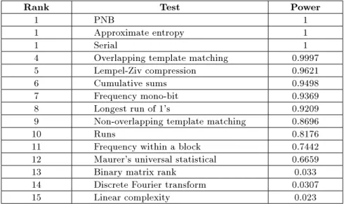
The NIST and the PNB tests are executed to eval-uate nonrandom sequences listed in Table B2. The power of each test resulted from each category is listed in Tables C1 to C3 and ranked decreasingly. The power is the proportion of sequences whose non-radnomness could be detected by the corresponding test.
We did not include the \Random Excursion Tests", as they do not output single P -value.
APPENDIX D Selected Histograms
Figure D1 represents the histogram resulted from executing the Algorithm on some sequences chosen from our sample in Table B1. For all sequences besides E(0), Algorithm 4 has been carried out using 10 as the depth of the start layer; for sequence E(0), The Next Bit histograms are shown, using 8 to 15 as the depth of the start layer.
Table C1. The power of tests in nding nonrandomness in JPEG sequences.
Rank Test Power
1 PNB 1
1 Approximate entropy 1
1 Serial 1
4 Overlapping template matching 0.9997 5 Lempel-Ziv compression 0.9621 6 Cumulative sums 0.9498 7 Frequency mono-bit 0.9369 8 Longest run of 1's 0.9209 9 Non-overlapping template matching 0.8696
10 Runs 0.8176
11 Frequency within a block 0.7442 12 Maurer's universal statistical 0.6659 13 Binary matrix rank 0.033 14 Discrete Fourier transform 0.0307 15 Linear complexity 0.023
Table C2. The power of tests in nding nonrandomness in GIF sequences.
Rank Test Power
1 PNB 1
1 Approximate entropy 1 1 Frequency within a block 1 1 Longest run of 1's 1
1 Serial 1
1 Maurer's universal statistical 1 7 Cumulative sums 0.9986 8 Overlapping template matching 0.9918 9 Frequency mono-bit 0.9823 10 Non-overlapping template matching 0.981 11 Lempel-Ziv compression 0.9756
12 Runs 0.9512
13 Discrete Fourier transform 0.6219 14 Binary matrix rank 0.1382 15 Linear complexity 0.1192
Table C3. The power of tests in nding nonrandomness in GZip Compressed sequences.
Rank Test Power
1 PNB 0.9904
2 Approximate entropy 0.9842
3 Serial 0.9786
4 Overlapping template matching 0.96 5 Maurer's universal statistical 0.9483 6 Frequency within a block 0.93 7 Non-overlapping template matching 0.9151 8 Cumulative sums 0.8015 9 Lempel-Ziv compression 0.77 10 Frequency mono-bit 0.7375 11 Longest run of 1's 0.7362
12 Runs 0.5802
13 Discrete Fourier transform 0.0331 14 Linear complexity 0.0246 15 Binary matrix rank 0.0237
Figure D1. Results of executing histogram test (Algorithm 4) on sample sequences. Each Histogram shows the number of occurrences of local nonrandomness w.r.t. the length of prediction block for dierent sequences of our sample.