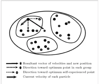
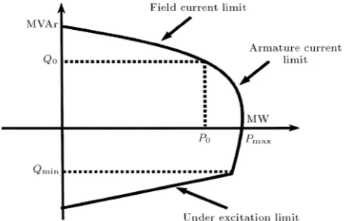
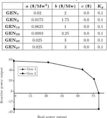
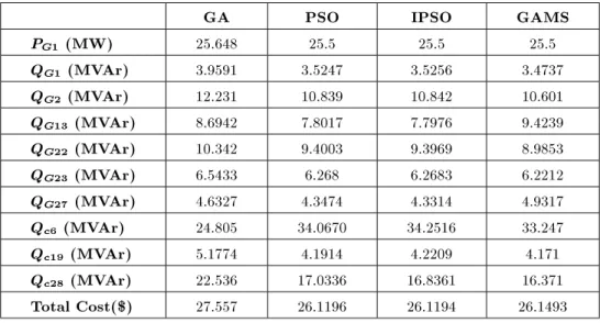
Particle Swarm Optimization Method for Optimal Reactive Power Procurement Considering Voltage Stability

Title A novel drug delivery system of intraperitoneal chemotherapy for peritoneal carcinomatosis using gelatin microspheres incorporating cisplatin.. Author(s) Gunji, Shutaro;

When Neighborcare Health at West Seattle High School is closed, students and their families are encouraged to call a Neighborcare Health clinic for medical, dental and mental

For example, [21] has offered a two-stage approach in which in the first phase, a new feature descriptor called maximum entropy feature descriptor (MEFD) is used

In order to test the ability of the mini-SEA to distinguish amnestic bvFTD patients from Alzheimer’s disease, the bvFTD group was divided in two subgroups

For example, Extract 5 displays a continuing (chronology) positive (evaluation) initiative for the environment (categorization). Since CEO Statements are an overview

In addition, Linde supplies tried-and-tested plants and process technologies for treating raw carbon dioxide from a wide range of industrial processes.. These include

Approximately 15% of asthmatics and 34% of the patients Attacks of asthma precipitated by aspirin like drugs are with asthma and concomitant rhinosinusitis were unaware due to

Additional research should address lumbar flexion and extension AROM between a control group of non-runners and runners; the current study demonstrated a.. marginally