Entropy Generation Analysis of a Flat Plate Boundary Layer with VariousSolution Methods

Entropy Generation Analysis of a Flat Plate

Boundary Layer with Various Solution Methods

J.A. Esfahani

and M. Malek Jafarian 1

Steady state boundary layer equations over a at plate with a constant wall temperature can be solved by an integral solution (with three proles for velocity and temperature), a similarity solution (exact) and a Blasius series solution. The analysis of entropy generation for each solution is carried out. The results show that the exact solution (similarity) is the one that minimizes the rate of total entropy generation in the boundary layer. Then, the Blasius solution has the least entropy generation of all. The bell-shaped prole (sinus prole) in the integral solution generates less entropy than the piecewise linear prole, consequently. So, with this method, if the exact solution for a specied problem were not available, one could evaluate the approximate solutions and recognize the best one among them. By introducing a new non-dimensional number (Ej number), which is the ratio of thermal entropy to friction entropy generation, one can recognize which of them is dominant in the boundary layer. Also, it is observed that variation of the total entropy generation is the same as the variation of boundary layer thickness, so, the non-dimensional total entropy generation for various solutions is constant.

INTRODUCTION

Heat transfer phenomena are always accompanied by entropy generation, hence, by the one-way destruction of available work. Therefore, it makes good engineering sense to focus on the irreversibility of heat transfer processes and try to understand the function of the entropy generation mechanism. For example, good heat exchanger design means, ultimately, an ecient thermodynamic performance, which is the least gener-ation of entropy or least destruction of available work (exergy) in the power/refrigeration system incorporat-ing the heat exchanger 1].

The art of adjusting the convection process so that it destroys the least available work (subject to various system constraints) is the focus of the applied eld of entropy generation minimization. Fowler and Bejan used a thermo-economic analysis to study the optimal sizes of bodies with specied external forced convection heat transfer 2]. Shuja and Zubair presented a thermo-economic design and optimization of ns with a con-*. Corresponding Author, Department of Mechanical Engi-neering, Ferdowsi University of Mashad, Mashad, P.O. Box 91755-1111, I.R. Iran.

1. Department of Mechanical Engineering, Ferdowsi Uni-versity of Mashad, Mashad, P.O. Box 91755-1111, I.R. Iran.

stant cross-sectional area. This includes capital costs and irreversibility penalty costs 3]. Sahin investigated entropy generation of a laminar ow, owing in a tube with a constant wall temperature 4]. Also, Esfahani and Baghdar investigated the eect of tube diameter on the optimum length, in the heat transfer process, with constant wall temperature 5]. Walsh et al. developed a quick, simple and, relatively, accurate method for the prediction of entropy in steady, two-dimensional, incompressible, adiabatic boundary layer ows of tur-bomachines, which gives both the distribution and magnitude of the entropy generation rate 6]. Also, they presented a preliminary optimization analysis, in the laminar region of a non lm cooled turbine blade, which demonstrates the concept of how the entropy generation rate may be reduced by varying the boundary layer edge velocity distribution along the suction surface, whilst the work done by the blade is kept constant 7]. Grin et al. investigated the eect of Reynolds number, compressibility and free stream turbulence on a prole of the entropy generation rate. Increased free stream turbulence had a greater eect on the generated entropy. It was observed that the amount of entropy generated in the turbulent boundary layer was, approximately, equivalent for two turbulence levels at a comparable Reynolds number 8]. Bejan showed that the natural shape of the velocity and tem-perature proles of the two-dimensional turbulent jet

is the one that minimizes the total entropy generation rate 9].

In the present work, the objective is to draw attention to the natural shape of velocity and temper-ature proles, which minimize the total entropy gener-ation rate. Hence, boundary layer equgener-ations over a at plate with constant wall temperature were solved by an integral solution (with three proles for velocity and temperature), a Blasius series solution and a similarity solution (exact solution). Then, the rate of entropy generation for each solution is calculated. The results show that the exact velocity and temperature prole (similarity solution) is the one that minimizes the rate of total entropy generation. The bell-shaped proles (sinus prole) in the integral solution generates less entropy than the piecewise linear prole, consequently, being closer to the natural shape of the velocity and thermal proles. So, with this method, if the exact solution for a specied problem were not available, one could evaluate the approximate solutions and recognize the best one among them.

GOVERNING EQUATIONS

Consider the ow over a horizontal at plate (Figure 1). The governing equations of this physical problem are the steady state boundary layer equations:

@u @x

+@v @y

= 0 (1)

u @u @x

+v @u @y

= @2u @y2

(2)

u @T @x

+v @T

@y

=

@2T @y2

(3)

where the velocity changes from u = 0 to u = U 1 and the temperature changes from T = T

w to T = T

1 in a space situated relatively close to the solid wall 10]. There are various methods for solving boundary layer equations. Here, integral, Blasius and similarity solution methods are investigated. In the next section, these methods are briey reviewed.

Figure1. Velocity, temperature and entropy generation boundary layer along a at plate parallel to a uniform stream.

SOLUTION METHODS

Similarity Solution

In this method, by introducing the similarity solution parameter, the streamline function and the dimension-less similarity temperature prole as 10]:

=y r

U 1 x

(4)

= p

U 1

xF() (5)

T w

;T T

w ;T

1

=G() (6)

the similarity form of the boundary layer momentum and energy equations are obtained as:

F 000

+ 12FF 00= 0

(7)

1 PrG

00

+ 12FG 0 = 0

(8)

with the following boundary conditions: (

G=F =F

0= 0 at

= 0 GF

0

!1 as !1:

(9)

Blasius Series Solution

The solution of Equation 7 is obtained by Blasius, which satises the boundary conditions by the method of matched asymptotic expansions 11]. Esfahani et al. make use of a modal series with the aid of the following dimensionless parameter 12]:

u U

1 =f

0( )

T w

;T T

w ;T

1

=g() (10)

where the closed form off() is dened as: f() =

1 X n=0

B n

n+1

3n+2

(11)

is as the same as Equation 4 and: B

n=

;1 2(3n)(3n+1)(3n+2)

n;1 X k=0

(3k+1)(3k+2)B k

B n;k ;1

: (12) By replacingf() into Equation 8 and integration,g() andg

0(

) are obtained as: g

0(

) = Exp

; 1 2pr

1 X n=0

B n

n+1 3n+ 3

3n+3 ;1:22

! g() =

Z 1

0 g 0(

Integral Solution

Integrating the conservative form of the boundary layer equations from y = 0 to y = Y = max(

T) and substituting boundary conditions, yields the integral boundary layer equations 10]. Assuming that the shape of the longitudinal velocity and temperature proles are described by:

( u U1 =

f( ) 1 1 u

U1 = 1 1

(14)

( T

w ;T Tw;T1 =

f() 0 1 T

w ;T

Tw;T1 = 1 1

(15)

f is an unspecied prole shape function that varies from 0 to 1 and = y

=

y

T, where

and T are the velocity and thermal boundary layer thicknesses. Substituting these denitions into an integral boundary layer equation for momentum yields:

x

=a1Re ;1=2 x

: (16)

The numerical coecient,a1, depends on the particular guess made for the prole shape function, f 10]. Assuming that:

T

= (17)

where is a function of the Prandtl number only and is given by Equation 16. Based on these denitions and

T

(Pr>1) and substitution into the integral form of the energy equation, one can determine

T 10]. Assuming the simplest temperature prole, f() =, one has:

= Pr;1=3

: (18)

Other choices of prole shape, f(), will change the proportionality factor in Equation 18 only percentage points. The results for other prole shapes, f( ) and f(), are hinted at by Table 1.

Table 1 shows that the boundary layer thickness is varied with various prole shapes. It is observed that there is a wide dierence between the results. The proper velocity and temperature proles could be the ones that minimize the total entropy generation rate of a at plate boundary layer. Thus, by calculation of the total entropy generation for various solutions, the more accurate solution and natural shape of proles can be recognized. In the next section, the methods of entropy generation calculation for various solutions are discussed.

ENTROPY GENERATION

It is easy to show that the rate of a one-way destruction of useful work in an engineering system, Wlost, is directly proportional to the rate of entropy generation:

Wlost=T i

Sgen (19)

where T

i is the absolute temperature of the ambient reservoir (T

i= constant) 1]. Assuming a nite-size con-trol volume at an arbitrary point in a two-dimensional convection ow eld and applying the second law of thermodynamics, the mix entropy generation per unit time and per unit volume (S

000

gen) is 10]:

S 000

gen= k T2

"

@T @x

2 +

@T @y

2 #

+ T

( 2

"

@u @x

2 +

@ @y

2 #

+

@u @y

+@ @x

2 )

(20) where k and are the conductivity and viscosity of the uid. T represents the absolute temperature of the point where S

000

gen is being evaluated. Equation 20

illustrates the cooperation between viscous dissipation and imperfect thermal contact in the generation of entropy via convective heat transfer. The entropy generation (Equation 20) can be simplied by scale Table1. The impact of prole shape on various solutions of the laminar boundary layer including friction and heat transfer.

Prole Shapes

f

(

) or

(

)

a 1

=

x

Re

1=2 x

a 2

=

T x

Re

1=2 x

Pr

1=3

Pr

f

=

f

=

(3

;

2

)

f

= sin

2

4.80 4.65 0.968

Blasius Solution (18 Terms)

analysis for ow over a at plate with lengthL: @T @x T L @T @y T T ! @T @x hh @T @y @ @x U 1 L2 @u @y U 1 ! @ @x hh @u @y @u @x U 1 L @u @y U 1 ! @u @x hh @u @y (21)

where T = T w

;T

1 is the scale of temperature variation in the region

T

L. Thus, entropy generation can be simplied as:

S 000

gen= k T2 @T @y 2 + T @u @y 2 : (22)

As seen, entropy generation depends on the deter-mining of ow eld velocity and temperature. The rst term on the right hand side of Equation 22 is called thermal entropy generation and the second term is called friction entropy generation. On the other hand, velocity and temperature proles depend on the method of solution, which is reviewed in the previous section. In the next section, various methods of solution are evaluated by entropy generation and the accuracy of them is discussed.

Calculation of Entropy Generation with

Similarity Solution

Non-dimensional mix entropy generation (S 000

gen) is

in-troduced as follows: S

000

gen= S

000

gen

(k=x2)Re x

= S

000

gen

k(a1=)2

(23)

which is normalized of entropy generation by boundary layer thickness. Using the denition ofin Equation 5 to express the derivative of velocity and temperature as: @u @y =U 1 r U 1 x F 00 @T @y

=;T r U 1 x G 0 (24) then, by replacing them into Equation 22 and using Equation 23, non-dimensional mix entropy generation can be written in the following form:

S 000 gen= T T 2 G 02+

T

T

:Ec:Pr:F 002

(25)

where Ec is the Eckert number of the uid and is dened as below:

Ec= U2

1 C

p :T

(26)

T refers to local temperature as: T =T

w

;T:G(): (27)

Now, one can dene a non-dimensional parameter as below: Ej= T T

:Ec:Pr (28)

where it is the ratio of non-dimensional friction entropy generation per thermal entropy generation. To create theEjnumber, Equation 25 is rearranged as:

S 000 gen T T ;2 =G

02+ Ej:F

002 :

A largeEj number shows that friction entropy genera-tion is more than the thermal entropy generagenera-tion in the boundary layer and vice versa for a smallEj number.

Calculation of Entropy Generation with

Blasius Solution

By derivation from velocity and temperature proles dened in Equation 10, one has:

S 000 gen= T T 2 Exp ;Pr 1 X n=0 B n n+1 3n+ 3

3n+3 ;2:44

! + T T :Ec:Pr:

1 X n=0

(3n+1)(3n+2)B n n+1 3n !2 (29) where:

T =T w

;T:g(): (30)

Calculation of Entropy Generation with

Integral Solution

Using the denition of the velocity and temperature proles in Equations 14 and 15, one has:

S 000 gen= T T 2 Pr1=3

a2 @f @ !2 + T T :Ec:Pr:

1 a1 @f @ 2 (31) where: T =T

w

;T:f() (32)

and

T are obtained from Table 1 for various prole shapes.

It should be mentioned that all the results dis-cussed here are for air over a at plate with the follow-ing characteristics, unless the characteristics expressed are in the text:

= 15:8910 ;6 m

2

s = 184:610 ;7 N.s

m2 k= 26:310

;3 w

m.k Pr = 0:707 T

w= 320 K T

1= 300 K

U

1= 10 ms where T

w T

1 and U

1 are the wall temperature, the free stream temperature and the free stream velocity, respectively. Based on data mentioned above, the value of the Ej number is 0.054, where it explains that thermal entropy generation is higher than friction entropy generation in the boundary layer at these conditions.

RESULTS AND DISCUSSION

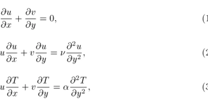
Figure 2 shows the distribution of friction, thermal and mixed entropy generation functions in the boundary layer (x = 0:5). The results are obtained by the Blasius series solution. The value of the friction term is very small (about one, near the wall), in contrast to the thermal term (about eleven, near the wall) and conrms the low Ej number described earlier. Also, it is seen that the ratio of friction to thermal entropy generation is about 0.1, which conrms the magnitude of the Ej number. Low values of the Ej number correspond to the low viscosity or low velocity of the uid. It is clear that by choosing a high viscosity or a high velocity, the contribution of the friction term will be signicant. This is shown in Figure 3, where the velocity of the uid is 100 m/s and other conditions are the same as earlier. At this condition,

Figure2. Distribution of entropy generation for Blasius solution (Tw= 320T1= 300U1= 10, heating).

Figure 3. Distribution of entropy generation for Blasius solution (T

w= 320 T

1= 300 U

1= 100, heating). the Ej number is 5.44, which can be supported by the ratio of 800_{100 in Figure 3. Thus, friction entropy}

generation is greater than thermal entropy generation. It is seen that the Ej number is a suitable parameter for evaluating the signicance of entropy generation components in the boundary layer. Also, three curves in Figures 2 and 3 have a maximum value at a point near the wall (not on the wall). This is observed for the other solutions too. Whenever the wall is cooled by the uid, the maximum and minimum values of the uid temperature are on the wall and the edge of the boundary layer, respectively. On the other hand, the slope of the temperature curve reduces from the wall to the edge of the boundary layer. Therefore, heat diusion decreases, so that the maximum value of the heat diusion will be on the wall (y = 0). Now, with attention to the denition of the entropy generation (dS

000

gen = Q

T ), marching in a

y direction will have a reduction in Q and T. Therefore, the denominator is trying to increase and the numerator is trying to decrease entropy generation, so that, near the wall, the dierence between the denominator and the numerator will have the least value. That will be the maximum entropy generation point.

Figure 4 shows the total entropy generation function, which is determined, as follows, for various solutions:

S 000

gen

total= max(

T) X y=0

L X x=0 S

000

gen: (33)

It is seen that the total entropy generation of the similarity solution is smaller than the other solutions and is the most for a linear prole (rough estimation) in the integral solution. Third order and sinus proles in the integral solution method are very close, so their proles have overlapped. The non-dimensional total

Figure4. Total entropy generation for various solutions (T

w= 320 T

1= 300 U

1= 10, heating). entropy generation function is dened as:

S 000

gen

total= max(

T) X y=0

L X x=0 S

000

gen (34)

and its distribution is shown in Figure 5. It is seen that the distribution of this parameter is constant for various solutions. This means that variation of total entropy generation is the same as variation of the boundary layer thickness. As observed in Figure 4, the non-dimensional total entropy of the similarity (exact) solution has the least value, then, the Blasius and integral solutions, respectively. The most value is for the linear prole in the integral solution.

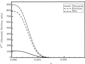
Distribution of thermal entropy generation for various solutions is compared in Figure 6 (x = 0:5). Entropy generation of the linear prole has minimum value on the wall in comparison to the other solutions. The reason is related to the slope of the temperature curves. The slope of the linear prole is less than the slope of the other proles (Table 1).

On the other hand, the value of k T

2 is constant for

Figure5. Non-dimensional total entropy generation for various solutions (Tw= 320T1= 300U1= 10, heating).

Figure6. Distribution of thermal entropy generation for various solutions (Tw= 320T1= 300U1= 10, heating). various solutions on the wall. Therefore, the thermal entropy generation of a linear prole will be less than the other solutions on the wall. But, moving from the wall (y > 0:0018), this trend will be reversed. At the edge of the boundary layer (y > 0:0042), a similar trend that is observed near the wall will appear. As seen from Table 1, the thermal boundary layer thickness for a linear prole is less than the other proles of integral, similarity and Blasius solutions. Therefore, the temperature gradient, as well as the thermal entropy generation, will reach zero at a shorter distance from the wall. Globally, thermal entropy generation has the least value for a similarity solution in the boundary layer thickness. Then, the Blasius solution, the integral solution with sinus and third order and linear proles have the smallest entropy generation, respectively.

Distribution of thermal entropy generation for various solutions is shown in Figure 7 (x = 0:5), where the wall temperature is less than the uid temperature (cooling conditions). It is seen that the maximum entropy generation occurs on the wall

Figure7. Distribution of thermal entropy generation for various solutions (Tw= 300T1= 320U1= 10, cooling).

(y = 0). Marching in ay direction (toward the wall), will have a reduction in T and an increase in Q. Therefore, the denominator and the numerator are trying to increase entropy generation, so that, on the wall, maximum entropy generation is obtained. But, in view of quantum, there is a similar trend to that of the heating case, shown in Figure 6.

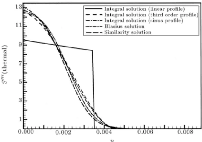
Figure 8 shows the friction entropy distribution in the boundary layer at the heating condition, which is similar to the thermal entropy generation shown in Figure 6. The same trend is observed near the wall and at the edge of the boundary layer, i.e., the minimum value on the wall and the entropy generation of the linear prole tends to zero faster than the other solutions. This is because of the small slope and small boundary layer thickness of the linear prole, in comparison with other proles, which reminds one that

T is constant on the wall in Equation 22.

Friction entropy generation at the cooling phe-nomena for various solutions is shown in Figure 9. The same trend observed in the thermal entropy generation of the cooling condition, is seen here. Globally, at the cooling phenomena, the similarity solution has the least value and, then, the Blasius solution.

The authors believe that because the similarity solution is the exact solution, its entropy generation is the least. Therefore, any prole, which produces entropy generation closer to the result of the similarity solution, is the most accurate estimation of all. Here, it is observed that the Blasius solution, with 18 terms, is a better estimation than the integral solutions.

CONCLUDING REMARKS

The entropy generation analysis of a at plate bound-ary layer with a constant wall temperature was carried out using three solution methods. Based on this work, the following conclusions can be drawn:

Figure8. Distribution of friction entropy generation for various solutions (Tw= 320T1= 300U1= 10, heating).

Figure 9. Distribution of friction entropy generation for various solutions (T

w= 300 T

1= 320 U

1= 10

cooling). The exact solution (similarity) produced less total

entropy generation than the other solutions. Then, the total entropy generation of the Blasius solution and the sinus prole in the integral method was the least, respectively

If there is not an exact solution for a problem, one can recognize the best solution, among approximate solutions, with an entropy generation analysis The variation of total entropy generation is the same

as the variation of boundary layer thickness The non-dimensional total entropy generation of all

solutions is constant

By introducing a non-dimensional number (Ej num-ber), one can recognize that one of the thermal en-tropy and friction enen-tropy generation is dominated in the boundary layer

For the heating phenomena (when the wall tem-perature is higher than the uid temtem-perature), the maximum entropy generation (thermal and friction) occurs near the wall (not on the wall). But, for the cooling phenomena, this maximum lies on the wall. From this work, one can recommend the analy-sis of entropy generation as procedure for evaluating solution methods in the eld of thermo-uid problems.

REFERENCES

1. Bejan, A., Entropy Generation Through Heat and Fluid Flow, chapter, 2, New York, USA (1982). 2. Fowler, A.J. and Bejan, A. \Correlation of optimal

sizes of bodies with external forced convection heat transfer", International Communication in Heat and Mass Transfer,21, pp 17-27 (Jan.-Feb. 1994). 3. Shuja, S.Z. and Zubair, S.M. \Thermoeconomic

opti-mization of constant cross-sectional area nes",ASME Journal of Heat Transfer,119(4), p 860 (1997).

4. Sahin, A.S. \Second law analysis of laminar viscous ow through a duct subjected to constant wall tem-perature", ASME Journal of Heat Transfer, 120, pp 76-83 (1998).

5. Abolfazli Esfahani, J.A. and Baghdar, F. \Entropy generation analysis of convective heat transfer through fully developed, laminar, viscous ow with a duct subjected to constant wall temperature", Journal of School of Engineering, Ferdowsi University of Mash-had,2, pp 85-98 (2001).

6. Walsh, E., Myose, R. and Davies, M. \A prediction method for the local entropy generation rate in a transitional boundary layer with a free stream pressure gradient",Stokes Research Institute, American Society of Mechanical Engineers, International Gas Turbine Institute, Turbo Expo (Publication) IGTI,3A, pp 637-646 (2002).

7. Walsh, E., Davies, M. and Myose, R. \An entropic minimization technique for turbine blade proles", American Society of Mechanical Engineers, Interna-tional Gas Turbine Institute, Turbo Expo (Publica-tion) IGTI,5A, pp 199-206 (2002).

8. Grin, P.C., O'Donnell, F.K., Davies, M. and Walsh, E. \The eect of Reynolds number, compressibility and free stream turbulence on prole entropy generation rate", American Society of Mechanical Engineers, In-ternational Gas Turbine Institute, Turbo Expo (Pub-lication) IGTI,5A, pp 61-69 (2002).

9. Bejan, A. \Thermodynamic of an isothermal ow: The two-dimensional turbulent jet",Int. J. Heat Mass Transfer,34, pp 407-413 (1991).

10. Bejan, A., Convection Heat Transfer, 2nd Ed., John Wiley & Sons, chapter 2 (1993).

11. Schlichting, G.H. \Boundary layer theory", Translated by Kestin, J., 4th Ed., McGrow Hill, pp 116-122 (1960).

12. Esfahani, J.A., Pariz, N. and Abdollahi, A. \Series solution of boundary layer along a plate by modal series approximation", Proceeding of the 4th Iranian Aerospace Society Conference, Amir Kabir University of Technology, pp 366-374 (Jan. 2003).