ISSN: 2251-8436 print/2322-1666 online
USING MODIFIED TWO-DIMENSIONAL
BLOCK-PULSE FUNCTIONS FOR THE NUMERICAL SOLUTION OF NONLINEAR TWO-DIMENSIONAL
VOLTERRA INTEGRAL EQUATIONS
FARSHID MIRZAEE∗, ELHAM HADADIYAN
Abstract. In this paper, the Modified two-dimensional block-pulse functions (M2D-BFs) are used as a new set of basis functions for expanding two-dimensional functions. The main properties of M2D-BFs are determined and an operational matrix for integration ob-tained. M2D-BFs are used to solve nonlinear two-dimensional Volterra integral equations of the first kind. Some theorems are included to show convergence and advantage of the method. Finally, numerical examples is presented to show the efficiency and accuracy of the method.
Key Words: Nonlinear two-dimensional Volterra integral equations, Block-pulse functions, Operational matrix.
2010 Mathematics Subject Classification:Primary: 45D05; Secondary: 65D30, 65R20.
1. Introduction
Many phenomena in physics and engineering fields give rise to a non-linear two-dimensional Volterra integral equation:
(1.1)
Z x
0
Z y
0
R(x, y, s, t, u(s, t))dtds=f(x, y); (x, y)∈D,
Received: 27 July 2013, Accepted: 15 January 2014. Communicated by D. Khojasteh Salkuyeh;
∗Address correspondence to Farshid Mirzaee; E-mail: [email protected]. c
2014 University of Mohaghegh Ardabili. 68
where u(s, t) is an unknown scalar valued function defined on district D= [0, T1)×[0, T2). The functionR(x, y, s, t, u) is given function defined
on
(1.2) W ={(x, y, s, t, u) : 0≤s≤x≤T1,0≤t≤y ≤T2}.
In this paper, we put
(1.3) R(x, y, s, t, u) =k(x, y, s, t)[u(s, t)]p, wherep is positive integer [7, 11].
Since any finite interval [a,b] can be transformed to [0,1] by linear maps, without any loss of generality, we consider [0,1) in replace of [0, T1) or [0, T2). While several numerical methods for approximating
the solution of one-dimensional Volterra integral equations are known, for two-dimensional only a few are discussed in the literature. The nu-merical solution of equations of the type of (1.1) seems to have first been considered by Bel’ tyukov and Kuznechikhina [2] where they proposed an explicit Rung-Kutta type method of order 3 without any convergence analysis. A bivariate cubic spline functions method of full continuity was obtained by Singh [15]. Brunner and Kauthen [3] introduced collocation and iterated collocation method for two-dimensional linear Volterra inte-gral equations. An asymptotic error expansion of the iterated collocation solution for two-dimensional linear and nonlinear Volterra integral equa-tions was obtained by Han and Zhang [6] and Guoqiang [4], respectively. Hadizadeh and Moatamedi [5] have investigated a differential transfor-mation approach for nonlinear two-dimensional Volterra integral equa-tions. Maleknejad et al. [9] used two-dimensional block-pulse functions to nonlinear integral equations. Babolian et al.[1] used two-dimensional triangular functions to nonlinear two-dimensional Volterra-Fredholm in-tegral equations. Mirzaee and Rafei [11] used the block by block method for the numerical solution of the nonlinear two-dimensional Volterra in-tegral equations.
Mirzaee and Hadadiyan [12] use the modified two-dimensional block-pulse functions method for the solutions mixed nonlinear Volterra- Fred-holm type integral equations. In the present paper, we apply modifica-tion of block-pulse funcmodifica-tions [12], to solve the nonlinear two-dimensional Volterra integral Eq. (1.1) with Eq. (1.2), and this is organized as fol-lows: In Section 2, we will introduce M2D-BFs and its properties. In Section 3, theorems are proved for convergence analysis. In Section 4, we will apply these sets of M2D-BFs for approximating the solution of
nonlinear Volterra integral equations. Numerical results are reported in Section 5. Finally , Section 6 concludes the paper .
2. M2D-BFs and their properties
Definition. An (m+1)2-set of M2D-BFs consists of (m+1)2functions which are defined over districtDas follows:
φi1,i2(x, y) =
1, (x, y)∈Di1,i2, i1, i2= 0(1)m
0, otherwise
, (2.1)
where
(2.2) Di1,i2 ={(x, y) :x∈Ii1,ε, y ∈Ii2,ε},
and
Iα,ε=
[0, h−ε), α= 0
[αh−ε,(α+ 1)h−ε), α= 1(1)m [1−ε,1), α=m
, (2.3)
wherem is arbitrary positive integer, andh= m1.
From Eq. (2.1), it is clearly that the M2D-BFs can be expressed by the two modified one-dimensional block-pulse functions (M1D-BFs): (2.4) φi1,i2(x, y) =φi1(x)φi2(y),
whereφi1(x) and φi2(y) are the M1D-BFs related to variables x and y,
respectively [9].
The M2D-BFs are disjointed with each other: φi1,i2(x, y)φj1,j2(x, y) =
φi1,i2(x, y), i1 =j1, i2=j2
0, otherwise , (2.5)
and are orthogonal with each other: (2.6)
Z 1
0
Z 1
0
φi1,i2(x, y)φj1,j2(x, y)dydx= (
4(Ii1,ε)4(Ii2,ε), i1=j1, i2 =j2
0, otherwise ,
where (x, y) ∈ D, i1, i2, j1, j2 = 0(1)m and 4(Ii1,ε) and 4(Ii2,ε) are
2.1. Vector forms. We can also define Φm,ε(x, y), the M2D-BFs vector, as follows:
(2.7)
Φm,ε(x, y) = [φ0,0(x, y), . . . , φ0,m(x, y), . . . , φm,0(x, y), . . . , φm,m(x, y)]T, were (x, y)∈Dand
(2.8) Φm,ε(x, y) = Φm,ε(x)⊗Φm,ε(y), and
(2.9) Φm,ε(x) = [φ0(x), φ1(x), . . . , φm(x)]T. Also we have:
Z x
0
Z y
0
Φm,ε(s, t)dtds=
Z x
0
Z y
0
Φm,ε(s)⊗Φm,ε(t)dtds=
Z x
0
Φm,ε(s)ds⊗
Z y
0
Φm,ε(t)dt=pm,ε⊗pm,ε=Pm,ε, (2.10)
wherepm,ε is operational matrix of 1D-BFs defined over [0,1), see [9]. From Eqs. (2.5) and (2.7) we have:
(2.11)
Φm,ε(x, y)ΦTm,ε(x, y) =
φ0,0(x, y) 0 . . . 0
0 φ0,1(x, y) . . . 0
..
. ... . .. ... 0 0 . . . φm,m(x, y)
.
Let X be a (m+ 1)2-vector by using Eq. (2.7) we will have: (2.12) Φm,ε(x, y)ΦTm,ε(x, y)X=XΦe m,ε(x, y),
whereXe =diag(X) is a (m+1)2×(m+1)2diagonal matrix. The disjoint
property of Φm,ε(x, y) also implies that for every (m+ 1)2×(m+ 1)2 -matrixA, we have:
(2.13) ΦTm,ε(x, y)AΦm,ε(x, y) =AbTΦm,ε(x, y),
where AbT is an (m+ 1)2-vector with elements equal to the diagonal
2.2. M2D-BFs expansions. An arbitrary functionf(x, y) defined over districtL2(D) can be expanded by the M2D-BFs as
f(x, y)'fm,ε(x, y) = m
X
i1=0
m
X
i2=0
fi1,i2φi1,i2(x, y)
=Fm,εT Φm,ε(x, y) = ΦTm,ε(x, y)Fm,ε, (2.14)
where
(2.15) Fm,ε= [f0,0, . . . , f0,m, . . . , fm,0, . . . , fm,m]T, andfi1,i2, are obtained as:
(2.16) fi1,i2 =
1
4(Ii1,ε)4(Ii2,ε) Z
Ii1,ε Z
Ii2,ε
f(x, y)dydx.
Similarly an arbitrary function of four variables,k(x, y, s, t), on dis-trict L2(D×D) may be approximated with respect to M2D-BFs such as:
(2.17) k(x, y, s, t)'ΦTm,ε(x, y)Km,εΦm,ε(s, t),
where Φm,ε(x, y) and Φm,ε(s, t) are M2D-BFs vector of dimension (m+ 1)2, and Km,ε is the (m+ 1)2×(m+ 1)2 M2D-BFs coefficients matrix.
3. Convergence analysis
In this sections, we show that the M2D-BFs method in the previous sections, is convergent and its order of convergence is O(km1 ). For our purposes we will need the following theorems.
Theorem 1.Let
(3.1) fm,ε(x, y) = m
X
i1=0
m
X
i2=0
fi1,i2φi1,i2(x, y),
and fori1, i2 = 0(1)(m) we have:
(3.2) fi1,i2 =
1
4(Ii1,ε)4(Ii2,ε)
Z 1
0
Z 1
0
f(x, y)φi1,i2(x, y)dxdy .
Then the criterion of this approximation is that the mean square error betweenf(x, y) and fm,ε(x, y) in the interval (x, y)∈D:
(3.3) =
Z 1
0
Z 1
0
reaches its minimum. Moreover, we have: (3.4)
Z 1
0
Z 1
0
f2(x, y)dxdy =
∞
X
i1=0
∞
X
i2=0
fi21,i2||φi1,i2(x, y)||
2.
Proof. Proof is like similar theorem in [8].
Theorem 2.Assumef(x, y) is continuous and is differentiable over dis-trict [−h,1+h]×[−h,1+h], andfm,εi(x, y);εi=
ih
k,fori= 0(1.1)(k−1), are correspondingly M2D-BFs(ε0)=2D-BFs, M2D-BFs (ε1),· · ·,
M2D-BFs(εk−1) expansions off(x, y) base on (m+ 1)2 M2D-BFs over district
D and
(3.5) fm,k(x, y) =¯ 1 k
k−1
X
i=0
fm,εi(x, y),
then for sufficient largem we have: (3.6) ||f(x, y)−f¯m,k(x, y)||∞≤
1 kmaxεi
||f(x, y)−fm,εi(x, y)||∞.
Proof. see [12]
Theorem 3. Let the representation error between f(x, y) and its two-dimensional block-pulse functions,fm(x, y) =fm,ε0(x, y) (M2D-BFs(ε0)=
2D-BFs), over the district D, as follows :
(3.7) e(x, y) =f(x, y)−fm(x, y). Then ||e(x, y)||=O(m1) and
(3.8) lim
m→+∞fm(x, y) =m→lim+∞fm,ε0(x, y) =f(x, y).
Proof. Proof is like similar theorem in [10].
Theorem 2 and 3 conclude that error estimation for M2D-BFs is
||e(x, y)||=O(km1 ).
Suppose that f(x, y) is approximated by (3.9) fm,εi(x, y) =
m
X
i1=0
m
X
i2=0
fi1,i2φi1,i2(x, y),
from [12] we have:
(3.10) lim
4. Method of solution
In this section, we solve two-dimensional nonlinear Volterra inte-gral equations of the first kind of the form Eq. (1.1) with Eq. (1.3) by using M2D-BFs.
We now approximate functionsu(x, y), f(x, y),[u(x, y)]pandk(x, y, s, t) with respect to M2D-BFs by the way mentioned in Section 2 as
(4.1)
u(x, y)'Um,εT Φm,ε(x, y),
f(x, y)'Fm,εT Φm,ε(x, y),
[u(x, y)]p 'ΦTm,ε(x, y)Um,ε,p,
k(x, y, s, t)'ΦTm,ε(x, y)Km,εΦm,ε(s, t),
where Φm,ε(x, y) is defined in Eq. (2.4), the vectors Um,ε, Fm,ε, Um,ε,p, and matrix Km,ε are M2D-BFs coefficients of u(x, y), f(x, y),[u(x, y)]p andk(x, y, s, t), respectively.
Lemma 1.Let (m+1)2-vectorsUm,εandUm,ε,pbe M2D-BFs coefficients ofu(x, y) and [u(x, y)]p, respectively. If
(4.2) Um,ε= [u0,0, . . . , u0,m, . . . , um,0, . . . , um,m]T, then
(4.3) Um,ε,p= [up0,0, . . . , up0,m, . . . , upm,0, . . . , upm,m]T, wherep≥1, is a positive integer.
Proof.(By induction) When p = 1, Eq. (4.3) follows at once from [u(x, y)]p =u(x, y). Suppose that Eq. (4.3) holds forp, we shall deduce it for (p+ 1). Since [u(x, y)]p+1 = u(x, y)[u(x, y)]p, from Eqs. (4.1), (2.12) it follows that
[u(x, y)]p+1=u(x, y)[u(x, y)]p 'Um,εT Φm,ε(x, y)ΦTm,ε(x, y)Um,ε,p =Um,εT Uem,ε,pΦm,ε(x, y).
(4.4)
Now by using Eq. (4.3) we obtain
Um,εT Um,ε,pe = [up0+1,0 , . . . , u0p+1,m, . . . , upm,+10, . . . , upm,m+1]T,
(4.5)
To approximate the integral part in Eq. (1.1), from Eq. (4.1) we get
Z x
0
Z y
0
k(x, y, s, t)[u(s, t)]pdtds'
(4.6)
Rx
0
Ry
0 Φ
T
m,ε(x, y)Km,εΦm,ε(s, t)ΦTm,ε(s, t)Um,ε,pdtds= ΦTm,ε(x, y)Km,ε R0xR0yΦm,ε(s, t)ΦTm,ε(x, y)Um,ε,pdtds=
ΦTm,ε(x, y)Km,εR0xR0yUm,ε,pΦm,ε(s, t)dtdse =
ΦTm,ε(x, y)Km,εUem,ε,p Rx
0
Ry
0 Φm,ε(s, t)dtds.
Now by using Eq. (2.10), we have: (4.7)
Z x
0
Z y
0
k(x, y, s, t)[u(s, t)]pdtds'ΦTm,ε(x, y)Km,εUem,ε,pPm,εΦm,ε(x, y),
in whichKm,εUem,ε,pPm,εis an (m+ 1)2×(m+ 1)2 matrix. By using Eq.
(2.13) we have:
Z x
0
Z y
0
k(x, y, s, t)[u(s, t)]pdtds'Ubm,ε,pT Φm,ε(x, y),
(4.8)
whereUm,ε,pb is and (m+ 1)2-vector with elements equal to the diagonal
entries of matrixKm,εUm,ε,pPm,ε. So, thee ith component of the column
vectorUbm,ε,p will be
i
X
j=1
pjikijvj; i= 1(1)(m+ 1)2, (4.9)
wherepij, kij andvj are the elements ofPm,ε, Km,ε, Um,ε,p, respectively, and
vj = (uj)p.
Applying Eqs. (4.1) and (4.6) in Eq. (1.1) with Eq. (1.3), we get
b
Um,ε,pT Φm,ε(x, y)'Fm,εT Φm,ε(x, y). (4.10)
Consequently we will have
After solving the above nonlinear system by using Newton-Raphson method, we can findUm,εand then
um,ε(x, y) =Um,εT Φm,ε(x, y). (4.12)
Then
u(x, y)'u¯m,k(x, y) = 1 k
k−1
X
i=0
um,εi(x, y),
(4.13)
where εi = ihk, i = 0(1)(k−1) is the estimation of the solution of two-dimensional Volterra integral equation of the first kind.
5. Numerical examples
In this section, the example is given to certify the convergence and error bound of the presented method. All results are computed by using a program written in the Matlab. The numerical experiments are carried our for the selected grid point which are proposed as (2−l ; l= 1,2,3,4,5,6) andmterms andktimes of modifications of the M2D-BFs series. The following problems have been tested.
Example 1. Consider the following linear two-dimensional Volterra integral equation [10]:
(5.1)
Z x
0
Z y
0
(sin(y+s)+sin(x+t)+3)u(s, t)dtds=f(x, y); (x, y)∈D,
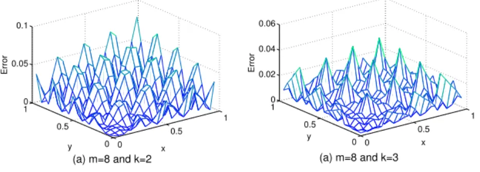
andf(x, y) is selected so that u(x, y) =cos(x+y) is the exact solution. Furthermore, Table 1 and Figures 1-2 illustrates the numerical results for this example.
0 0.5 1 0 0.5 1 0 0.02 0.04 0.06 x (a) m=8 and k=3 y Error 0 0.5 1 0 0.5 1 0 0.05 0.1 x (a) m=8 and k=2 y
Error
Figure 1. Absolute value of error, Example 1 withm= 8 andk= 2,3
0 0.5 1 0 0.5 1 0 0.01 0.02 0.03 0.04 x (a) m=16 and k= 2 y Error 0 0.5 1 0 0.5 1 0 0.01 0.02 0.03 x (b) m=16 and k= 3 y
Error
Figure 2. Absolute value of error, Example 1 withm= 16 andk= 2,3
Table 1: Numerical results of Example 1 with M2D-BFs
Nodes (x,y) Error for m=8 Error for m=16
(x,y)=2−l k=1(Ref.[10]) k=2 k=3 k=1(Ref.[10]) k=2 k=3
l= 1 0.085303 0.048609 0.035575 0.042396 0.023996 0.017469
l= 2 0.052873 0.029492 0.021487 0.025605 0.014216 0.010271
l= 3 0.045225 0.019710 0.012312 0.013869 0.007682 0.005582
l= 4 0.003428 0.007026 0.000477 0.011432 0.004991 0.003125
l= 5 0.002421 0.000779 0.000313 0.000863 0.001769 0.000118
l= 6 0.003886 0.002244 0.001778 0.000602 0.000193 0.000077
Example 2. Consider the following nonlinear two-dimensional Volterra integral equation [10]:
(5.2)
Z x
0
Z y
0
where
(5.3) f(x, y) = 1 45xy(9x
4+ 10x2y2+ 9y4).
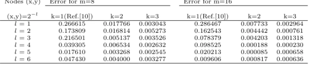
The exact solution is u(x, y) = x2 +y2. Furthermore, Table 2 and
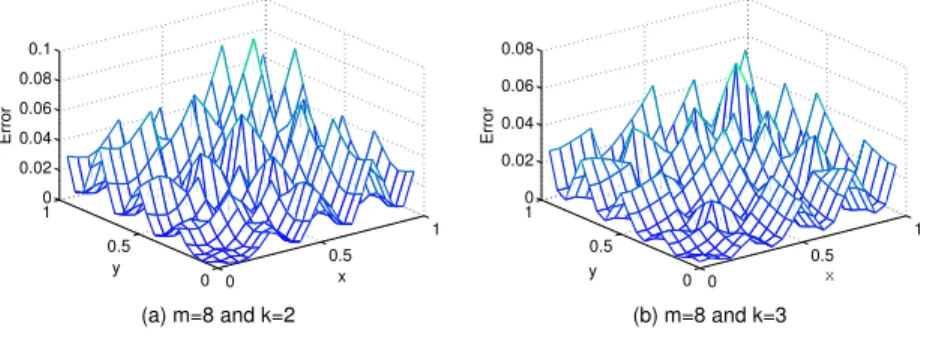
Figures 3-4 illustrates the numerical results for this example.
0
0.5 1 0
0.5 1 0 0.02 0.04 0.06 0.08 0.1
x
(a) m=8 and k=2
y
Error
0
0.5 1 0
0.5 1 0 0.02 0.04 0.06 0.08
x
(b) m=8 and k=3
y
Error
Figure 3. Absolute value of error, Example 2 withm= 8 andk= 2,3
0
0.5 1 0
0.5 1 0 0.01 0.02 0.03 0.04
x (b) m=16 and k= 3 y
Error
0
0.5 1 0
0.5 1 0 0.02 0.04 0.06
x (a) m=16 and k= 2 y
Error
Table 2: Numerical results of Example 2 with M2D-BFs
Nodes (x,y) Error for m=8 Error for m=16
(x,y)=2−l k=1(Ref.[10]) k=2 k=3 k=1(Ref.[10]) k=2 k=3
l= 1 0.266615 0.017766 0.003043 0.286467 0.007733 0.002964
l= 2 0.173809 0.016814 0.005273 0.162543 0.004442 0.000761
l= 3 0.216501 0.005137 0.003526 0.078379 0.004203 0.001318
l= 4 0.039305 0.006534 0.002632 0.098525 0.000188 0.000230
l= 5 0.017610 0.003268 0.002545 0.020213 0.000085 0.000658
l= 6 0.047430 0.004000 0.003277 0.009606 0.000817 0.000636
6. Conclusion
In this paper we have worked out a computational method for ap-proximate solution of nonlinear two-dimensional Volterra integral equa-tions of the first kind, based on the expansion of the solution as series of M2D-BFs. This method converts a nonlinear two-dimensional Volterra integral equation whose answer are the coefficients of M2D-BFs expan-sion of the solution of nonlinear two-dimenexpan-sional Volterra integral equa-tion. Note that the find system extracted from the nonlinear equations will be nonlinear and proper technique such Newton-Raphson method could be applied. This method can be easily extended and applied to nonlinear two-dimensional Volterra integral equations of the second kind and nonlinear two-dimensional Fredholm integral equations.
Acknowledgments
The authors wish to thank the referee for his (her) helpful comments
References
[1] E. Babolian, K. Maleknejad, M. Roodaki and H. Almasieh, Two-dimensional triangular functions and thire applications to nonlinear 2D Volterra-fredholm integral equations, Computers and Mathematics with Applications,60 (2010), 1711–1722.
[2] B. A. Bel’ tyukov and L. N. Kuznechikhina,A Rung-Kutta method for solution of two-dimensional nonlinear Volterra integral equations, Differential Equations,
12(1976) 1169–1173.
[3] H. Brunner and J.P. Kauthen, The numerical solution of two-dimensional Volterra integral equations by collocation and iterated collocation, IMA Journal of Numerical Analysis,9(1989) 47–59.
[4] H. Guoqiang, K. Hayami, K. Sugihara and W. Jiong, Extrapolation method of iterated collocation solution for two-dimensional nonlinear Volterra integral equa-tion, Applied Mathematics and Computation,112(2000) 49–61.
[5] M. Hadizadeh and N. Moatamedi,A new differential transformation approach for two-dimensional Volterra integral equations, International Journal of Computer Mathematics,84(2007) 515–529.
[6] G.Q. Han and L.Q. Zhang, Asymptotic error expansion of two-dimensional Volterra integral equation by iterated collocation, Applied Mathematics and Com-putation,61(1994) 269–285.
[7] R. Hanson and J. Phillips,Numerical solution of two-dimensional integral equa-tions using linear elements, SAIM Journal on Numerical Analysis, 15 (1978) 113–121.
[8] Z. H. Jiang and W. Schaufelberger,Block Pulse functions and their applications in control systems, Spriger-Verlag, Berlin (1992).
[9] K. Maleknejad and B. Rahimi, Modification of block pulse functions and their application to solve numericaliy Volterra integral equation of the first kind, Com-munications in Nonlinear Science and Numerical Simulation, 16 (2011) 2469– 2477.
[10] K. Maleknejad, S. Sohrabi and B. Baranji,Application of 2D-BPFs to nonlinear integral equations, Communications in Nonlinear Science and Numerical Simula-tion,15(2010) 527–535.
[11] S. Mckee, T. Tang and T. Diago, An Euler-type method for two-dimensional Volterra integral equations of the first kind, IMA Journal of Numerical Analysis,
20(2000) 423–440.
[12] F. Mirzaee and E. Hadadiyan, Approximate solutions for mixed nonlinear Volterra-Fredholm type integral equations via modified block-pulse functions, Journal of the Association of Arab Universities for Basic and Applied Sciences,
12(2012) 65–73.
[13] F. Mirzaee and Z. Rafei,The block by block method for the numerical solution of the nonlinear two-dimensional Volterra integral equations, Journal of King Saud University Science,23(2011) 191–195.
[14] W. Rudin,Principles of mathematical analysis, Singapore: McGraw-Hill, (1976). [15] P. Singh,A note on the solution of two-dimensional Volterra integral equations
by spline, Indian Journal of Mathematics,18(1979) 61–64.
Farshid Mirzaee
Department of Mathematics, Faculty of Science, University of Malayer, 65719-95863, Malayer, Iran
Email: [email protected]; f.mirzaee @iust.ac.ir.
Elham Hadadiyan
Department of Mathematics, Faculty of Science, University of Malayer, 65719-95863, Malayer, Iran