Sharif University of Technology
Scientia IranicaTransactions B: Mechanical Engineering www.scientiairanica.com
Research Note
Numerical solution of general boundary layer problems
by the method of dierential quadrature
S.A. Eftekhari
and A.A. Jafari
Department of Mechanical Engineering, K.N. Toosi University, Tehran, P.O. Box 19395-1999, Iran. Received 4 August 2011; received in revised form 18 August 2012; accepted 23 March 2013
KEYWORDS Dierential
Quadrature Method (DQM);
Blasius ow; Sakiadis ow; Falkner-Skan ow; MHD Falkner-Skan ow;
Jeery-Hamel ow; Unsteady two-dimensional ow; Unsteady three-dimensional MHD ow.
Abstract.Accurate numerical solutions to some boundary layer equations are presented for boundary layer ows of incompressible Newtonian uid over a semi-innite plate. The Dierential Quadrature Method (DQM) is rst used to reduce the governing nonlinear dierential equations to a set of nonlinear algebraic equations. The Newton-Raphson method is then employed to solve the resulting system of nonlinear algebraic equations. The proposed formulation is applied here to solve some boundary layer problems, including Blasius, Sakiadis, Falkner-Skan, magnetohydrodynamic (MHD) Falkner-Skan, Jeery-Hamel, unsteady two-dimensional and three-dimensional MHD ows. A simple scheme is also presented for solving the Blasius boundary layer equation. In this technique, the Blasius boundary value problem is rst converted to a pair of nonlinear initial-value problems and then solved by a step-by-step DQM. The accuracy and eciency of the proposed formulations are demonstrated by comparing the calculated results with those of other numerical and semi-analytical methods. Accurate numerical solutions are achieved using both formulations via a small number of grid points for all the cases considered.
c
2013 Sharif University of Technology. All rights reserved.
1. Introduction
Laminar boundary layers have long been the subject of numerous studies, since they play an important role in understanding the main physical features of boundary-layer phenomena. Generally, no closed-form solutions are available for laminar boundary value problems. Therefore, many researchers have resorted to various numerical or semi-analytical methods to solve such problems. However, it is not an easy task to solve, nu-merically, such types of problem. The main issue is how to model such problems (with innite or semi-innite domains) by a method of approximation with nite grid spacing. To tackle this issue in mathematical modeling *. Corresponding author. Tel.: +98-0919-4618599;
Fax: +98 21 88674748.
E-mail address: [email protected] (S.A. Eftekhari)
of the problem, one can apply the innite boundary condition at a nite boundary placed at a large distance from the object (i.e., truncated boundary). This, however, begs the question of what is a 'large distance' and, obviously, substantial errors may arise if the boundary is not placed far enough away. On the other hand, pushing this out excessively far necessitates the introduction of a large number of grids to model regions of relatively little interest to the analyst. Obviously, when a low-order numerical method is used for the solution of boundary layer problems, many calculations should be done to accurately predict the location of the truncated boundary. Therefore, to accurately predict the location of the truncated boundary and to reduce the computational time, higher-order numerical methods should be used to model the boundary layer problems.
The Blasius boundary layer is an example of two-dimensional boundary layer problems. The Blasius
problem models the behavior of a two-dimensional steady state laminar viscous ow of an incompressible uid over a semi-innite at plate. The governing dierential equation of the problem is (see [1] and Appendix A.1):
f000() +1
2f()f00() = 0; 0 1; (1)
where and f() are the dimensionless coordinate and stream function, respectively. The boundary conditions for Eq. (1) are:
f(0) = f0(0) = 0; f0(1) = 1: (2)
The problem was rst solved by Blasius using a series expansions method. But the proposed semi-analytic series solution does not converge at all. In fact, the obtained semi-analytic solution is valid only for small values of (i.e., the series solution converges only within a nite interval [0; 0], where 0 is an
unknown constant which can be determined numeri-cally or analytinumeri-cally). Howarth [2] solved the Blasius equation numerically and found 0 1:8894=0:33206.
Furthermore, Asaithambi [3] solved the Blasius equa-tion more accurately and obtained this number as 0 1:8894=0:332057336. Due to the limitation of the
Blasius power series solution, many attempts have been made to obtain solutions which are valid on the whole domain of the problem. Some researchers have solved the problem numerically and some semi-analytically. Applying the Homotopy Analysis Method (HAM) [4], Liao obtained an analytic solution for the Blasius equation which is valid in the whole region of the problem [5,6]. Using the Variational Iteration Method (VIM) [7], He constructed a ve-term approximate-analytic solution for the Blasius equation which is also valid for large values of [8]. However, the solutions obtained were not very accurate. The Adomian De-composition Method (ADM) has also been used by some researchers to nd semi-analytic solutions for the Blasius equation [9-11]. A homotopy perturbation solution to this problem was presented by He [12,13]. Kou [14], Fang et al. [15], Cortell [16], Ahmad [17], Parand and Taghavi [18], Ahmad and Al-Barakati [19] and Parand et al. [20] also solved the Blasius problem using various numerical and semi-analytical methods.
The Blasius boundary layer equation may be viewed as a special case of the Falkner-Skan equation, which has the form (see Appendix A.2):
f000() +
0f()f00() + 1 f0()2= 0;
0 1; (3)
where is constant. The Falkner-Skan equation arises in the study of laminar boundary layers exhibit-ing similarity. The solutions of the one-dimensional
third-order boundary-value problem described by the well-known Falkner-Skan equation are the similarity solutions of two-dimensional incompressible laminar boundary layer equations [3]. Physically, the Falkner-Skan equation describes two-dimensional ow over stationary impenetrable wedge surfaces of included angle , which limits to a at plate, and the Blasius solution, as approaches zero. The solutions of the Falkner-Skan equation corresponding to > 0 have become known as accelerating ows, those correspond-ing to = 0 are called constant ows, and those corresponding to < 0 are known as decelerating ows with separation. Physically relevant solutions exist only for 0:19884 < 2. The closed form solution for the behavior of the nonlinear two-point Falkner-Skan boundary value problem does not exist, so, such a problem has been studied by approxi-mate numerical and semi-analytical methods, such as the shooting method [21-23], the spline collocation procedure [24], the nite dierence method [25,26], the nite element method with linear interpolation functions [27], ADM [28,29], HAM [30,31], the coupling quasilinearization method and the spline method [32], the Fourier series method [33] and the collocation method [34].
When the Falkner-Skan boundary layer ow is subjected to a magnetic eld, the governing dierential equation for the boundary layer can be expressed as (see [35] and Appendix A.3):
f000()+f()f00()+(1 f0()2) M2(f0() 1)=0;
0 1; (4)
with the same boundary conditions as the Blasius equa-tion (see Eq. (2)), where and M are constants. The study of ows of this type is known as Magnetohydro-dynamics or MHD for short. Such ows are of strong interest in the design and analysis of power generators, pumps, accelerators, electrostatic lters, droplet lters, heat exchangers, reactors and the like. MHD boundary layer ows have been studied by several researchers. Yih [36] and Ishak et al. [37] transformed the partial dierential boundary layer equations into non-similar boundary layer equations and a system of ordinary dierential equations, respectively, and then used the Keller box method to solve them. Abbasbandy and Hayat [35,38] solved MHD boundary layer ow by modied HAM and Hankel-Pade methods, respectively. Most recently, Parand et al. [39] found a solution for the problem by the pseudospectral method.
On the other hand, dierent from Blasius, Falkner and Skan, Sakiadis [40] considered the boundary layer ow on a moving (or stretching) at surface in a quiescent ambient uid. He found the same Ordinary Dierential Equation (ODE) as Blasius, but the bound-ary conditions were dierent. The boundbound-ary conditions
for the Sakiadis at-plate ow problem are (see [40] and Appendix A.4):
f(0) = f0(1) = 0; f0(0) = 1: (5)
Tsou et al. [41] made an experimental and theoretical treatment of this problem to prove that such a ow is physically realizable. Based on the fact that a single ODE governs both Blasius and Sakiadis ow, some researchers discussed both two classical boundary-layer ows simultaneously in a single paper and provided an interesting comparison of the problems [42-44]. One of their conclusions was that the skin friction (f000 = )
is about 34% higher for the Sakiadis ow compared to the Blasius case. Later, Bataller [45] solved the Blasius and Sakiadis equations more accurately and obtained this value as 33.63%. Dierent eects, such as suction/blowing, and radiation, etc., on the above mentioned classes of ow are discussed in most recent papers by Ishak et al. [46], Fang [47] and Cortell [48]. Moreover, recent research into boundary layer ow and heat/mass transfer on a moving at plate in a parallel stream has also been carried out by Cortell [49] and Ishak et al. [50].
As pointed out by Sakiadis [40], the non-dimensional governing dierential equations for bound-ary layer ows on moving plates are exactly the same as those on xed plates. Following this idea, one can easily formulate and solve the Falkner-Skan boundary layer ow and MHD Falkner-Skan boundary layer ow on moving or stretching plates. It can be easily veried that the boundary conditions for Falkner-Skan ow and MHD Falkner-Skan ow on moving or stretching plates are the same as those given in Eq. (5). With this in mind, Elgazery [28], Liao [51,52], Rashidi [53], Bognar [54] and Fathizadeh et al. [55] solved the Skan boundary layer problem or MHD Falkner-Skan boundary layer problem using various approxi-mate (or semi-analytic) methods.
In all the above-mentioned studies, steady two dimensional boundary layer ows were considered. Compared to the large amount of research study into two dimensional boundary layer ows, the published work on three dimensional boundary layer ows is limited. Only few works based on the steady boundary layer theory have been carried out [56-58]. The governing non-dimensional dierential equations for an unsteady two dimensional boundary layer developed by an impulsively stretching plate in a constant pressure viscous ow is (see [59] and Appendix A.5):
f;+12(1 )f;+ [ff; f;2]=(1 )f;;
0 1; 0; (6)
subject to the boundary conditions:
f(0; ) = f;(1; ) = 0; f;(0; ) = 1; (7)
where a subscript comma denotes dierentiation. Liao [59] solved the above problem using the per-turbation method and HAM. The unsteady three-dimensional MHD boundary layer ow and heat trans-fer due to an impulsively stretched plane surface were studied using HAM by Xu et al. [60] and Kumari and Nath [61]. The boundary layer equations, based on the conservation of mass, momentum and energy, governing unsteady three-dimensional ow and heat transfer on a stretching surface in the presence of a magnetic eld, can be expressed in dimensionless form as (see [60,61] and Appendix A.6):
f;+12(1 )f;+ [(f + s)f; f;2 Mf;]
= (1 )f;;
0 1; 0; (8)
s;+12(1 )s;+ [(f + s)s; s2; Ms;]
= (1 )s;; (9)
g;+12Pr(1 )g;+Pr(f +s)g;=Pr(1 )g;;
(10) subject to the boundary conditions:
f(0; )=s(0; )=g(1; )=f;(1; )=s;(1; ) = 0;
g(0; ) = f;(0; ) = 1; s;(0; ) = c; (11)
where c is a positive constant, M is the magnetic parameter and Pr is the Prandtl number.
On the other hand, dierent from Blasius, Falkner, Skan and Sakiadis, Jeery and Hamel [62,63] introduced the problem of the uid ow through convergent-divergent channels. This problem has many applications in aero-space, chemical, civil, environmen-tal, mechanical and bio-mechanical engineering, as well as in understanding rivers and canals. Jeery-Hamel ows are interesting models of the phenomenon of the separation of boundary layers in divergent channels. These ows have revealed a multiplicity of solutions, richer perhaps than other similarity solutions of the Navier-Stokes equations, because of the dependence on two non-dimensional parameters i.e. the ow Reynolds number and channel angular widths [64]. The governing non-dimensional dierential equation for the Jeery-Hamel ow is (see Appendix A.7):
f000() + 2Ref()f0() + (4 Ha)2f0() = 0;
subject to the boundary conditions:
f(0) = 1; f0(0) = 0; f(1) = 0; (13)
where Re is the Reynolds number, Ha is the Hartmann number and is the angle of chan-nel [64]. Closed form solutions for Jeery-Hamel ow cannot be found in the literature, so, such boundary layer problems have to be mainly stud-ied by approximate (or semi-analytic) methods, such as the Hermite-Pade approximation method [64], ADM [65,66], He's semi-analytical methods [67], HAM [68,69], the Optimal Homotopy Asymptotic Method (OHAM) [70], HAM, the Homotopy Pertur-bation Method (HPM) and the Dierential Transfor-mation Method (DTM) [71].
From a review of existing literature [1-71], it is found that most researchers are interested in the anal-ysis of boundary layer problems using semi-analytical methods (although in some papers, the researchers call their approximate method an analytic one). Moreover, one cannot nd a single paper in the literature that includes all types of boundary layer problem. In spite of the enormous numerical eort, a truly simple, yet numerically accurate and robust algorithm is still missing. From the review of the schemes proposed in [4-71], two general limitations may be observed:
1. The proposed approximate-analytic methods can-not yield accurate solutions when a rather small number of solution terms are used;
2. Many calculations should be done to construct the resulting semi-analytic solutions, which increase the CPU time considerably, especially when a large number of solution terms are to be used.
The above-mentioned limitations can be elimi-nated using higher-order methods, such as the Dieren-tial Quadrature Method (DQM). The DQM, which was rst introduced by Bellman and his associates [72] in the early 1970s, is an alternative ecient discretization technique for solving directly the governing dieren-tial equations in engineering and mathematics. Its central idea is to approximate the derivative of a function, with respect to a space/time variable at a given discrete point, by a weighed linear summation of the function values at all of the discrete points in the domain of that variable. Compared to the low-order methods, such as the nite element and nite dierence methods, the DQM can generate numerical results with a higher-order of accuracy by using a considerably smaller number of discrete points and, therefore, requiring relatively little computational ef-fort. Another particular advantage of the DQM is its ease of use and implementation. Since its introduction, the DQM has been successfully applied to many areas in engineering and mathematics [73]. Details of this
method and references of application of the DQM to various problems may be found, for example, in the review paper by Bert and Malik [74]. More recently, the DQM has been successfully applied to initial-value problems in structural dynamics [75-80]. It has been found that the DQ time integration scheme is reliable, computationally ecient and also suitable for time integrations over a long time duration. Most recently, the DQM has been successfully combined with other approximate methods, such as the Ritz method [81-83] and nite element method [84], and applied to free and forced vibration, and buckling problems of rectangular plates.
The DQM has also been successfully applied to simple boundary layer problems such as the Blasius and Sakiadis equations [85,86]. Liu and Wu [85] proposed the use of Hermite functions as trial functions to determine the weighting coecients in the DQM and called their method the Generalized Dierential Quadrature Method (GDQM). They applied their method to Blasius and Onsager equations and reported accurate solutions. The emphasis on their study was placed on implementing multiple boundary conditions in the solution process. However, as we will show in this paper, the conventional DQM can also produce highly accurate solutions for general boundary layer problems without any diculty and, thus, there is no need to use any other scheme, such as one proposed by Liu and Wu [85], to implement boundary conditions in the DQ solution of boundary layer equations. On the other hand, Girgin [86] proposed an iterative DQM for solving Blasius and Sakiadis boundary layer problems and called their method the Generalized Iterative Dierential Quadrature Method (GIDQM). However, as we know, the proposed method (GIDQM) is, in fact, a direct application of the DQM to boundary layer problems. Moreover, the accuracy and capability of the GIDQM has not been challenged through the solution of general boundary layer problems.
It can be seen that a general formulation based on the DQM for solving general boundary layer problems is still missing. Therefore, the present investigation is devoted to presenting an iterative DQM for the solution of general boundary layer equations. At rst, we present a general formulation for solving Bla-sius, Sakiadis, Falkner-Skan, MHD Falkner-Skan and Jeery-Hamel boundary layer problems. An iterative DQM will then be presented for solving unsteady two-dimensional and three-dimensional boundary layer problems. Finally, a simple scheme is proposed for solving Blasius boundary layer equation. In this technique, the Blasius boundary value problem is rst converted to a pair of initial-value problems [87] and then solved by a step-by-step DQM. A comparison is also made with the conventional fourth-order Runge-Kutta method (RK4).
2. Dierential quadrature method
Let f(; ) be a solution of a partial dierential equa-tion, 1; 2; ; n be a set of sampling points in the
-direction and 1; 2; ; mbe that in the -direction.
According to the DQM, the rst-order derivatives, f;
and f;, at a sample point (i, j) can be expressed by
the quadrature rules as [72-74]: f;(i; j) =
n
X
k=1
A(1)ikfkj;
i = 1; 2; :::; n; (14)
f;(i; j) = m
X
l=1
Bjl(1)fil;
j = 1; 2; :::; m; (15)
where fij = f(i; j), A(1)ik are the rstorder
-derivative weighting coecients associated with the = i point, and, similarly, Bjl(1) are the rst-order
-derivative weighting coecients associated with the = j point. A(1)ik and Bjl(1) are given by [73]:
A(1)ik = 8 > > > > > > < > > > > > > :
M(1)( i)
(i k)M(1)(k) i 6= k;
i; k = 1; 2; ; n Pn
j=1;j6=iA(1)ij i = k;
i = 1; 2; ; n
(16)
Bjl(1)= 8 > > > > > > < > > > > > > :
M(1)( j)
(j l)M(1)(l) j 6= l;
j; l = 1; 2; ; m Pm
i=1;i6=jBji(1) j = l;
j = 1; 2; ; m
(17)
where M(1)() and M(1)() are dened as:
M(1)( i) =
n
Y
j=1;j6=i
(i j);
M(1)( i) =
m
Y
j=1;j6=i
(i j): (18)
The weighting coecients of the rth-order derivative (r 2) may be obtained through the following relationships:
A(r)ik = 8 > > > > > > > < > > > > > > > : r
A(r 1)ii A(1)ik A(r 1)ik
(i k)
i 6= k;
i; k =1; 2; ; n Pn
j=1;j6=iA(r)ij i = k;
i = 1; 2; ; n (19)
Bjl(r)= 8 > > > > > > > < > > > > > > > : r
Bjj(r 1)B(1)jl B(r 1)jl
(j l)
j 6= l;
j; l =1; 2; ; m Pm
i=1;i6=jBji(r) j = l;
j = 1; 2; ; m (20)
In this study, the sampling points are taken nonuni-formly spaced, and are given by the following equa-tions: i= 2 1 cos (i 1) n 1
; i = 1; 2; ; n; (21) i= 2 1 cos (i 1) m 1
; i = 1; 2; ; m; (22) where and are problem boundaries in and
-directions, respectively.
3. General formulation for steady
two-dimensional boundary layer problems The Blasius, Sakiadis, Skan, (MHD) Falkner-Skan and Jeery-Hamel boundary layer problems all can be described by the following general nonlinear third-order boundary value problem:
f000() + a
1f()f00() + a2f()f0() + a3f0()2
+ a4f0() + a5= 0; 0 ; (23)
subject to the boundary conditions:
f(0)=b1; f0(0)=b2; f()=b3; =1;
(24) for the Jeery-Hamel boundary layer problem, and:
f(0)=b1; f0(0)=b2; f0()=b3;
=1; (25)
for other boundary layer problems. where ai, bj (i =
1; ; 5; j = 1; 2; 3) are constants.
For the DQ solution of the system equations, Eqs. (23) though (25), rst, the requisite quadrature
rules for the rst, second and third-order derivatives are written from Eq. (14), as:
f0 i =
n
X
j=1
A(1)ij fj; fi00= n
X
j=1
A(2)ij fj;
f000 i =
n
X
j=1
A(3)ij fj; (26)
wherein: f0
i = f0(i); fi00= f00(i); fi000= f000(i);
fj = f(j); (27)
where n is the number of sampling points in the domain 0 .
Satisfying Eq. (23) at any sample point = i,
one has: f000(
i) + a1f(i)f00(i) + a2f(i)f0(i) + a3f0(i)2
+ a4f0(i) + a5= 0; i = 1; 2; ; n: (28)
Or: f000
i + a1fifi00+ a2fifi0+ a3(fi0)2+ a4fi0+ a5= 0;
i = 1; 2; ; n: (29)
Now, substituting the quadrature rules given in Eq. (26) into Eq. (29), the quadrature analog of the governing dierential equation is obtained as:
n
X
j=1
A(3)ij fj+ a1fi n
X
j=1
A(2)ij fj+ a2fi n
X
j=1
A(1)ij fj
+ a3
0 @Xn
j=1
A(1)ij fj
1 A
2
+ a4 n
X
j=1
A(1)ij fj
+ a5= 0; i = 1; 2; ; n: (30)
Eq. (30) can be written in matrix notation as: [A](3)ffg + a
1ffg
[A](2)ffg
+ a2ffg
[A](1)ffg
+ a3
[A](1)ffg[A](1)ffg
+ a4[A](1)ffg + a5frg = f0g; (31)
where:
ffg =f1 f2 fnT;
frg =1 1 1T: (32)
Using the quadrature rules, the quadrature analogs of boundary conditions for the Jeery-Hamel boundary layer equation are obtained as:
f1= f(1) = b1;
f0
1= f0(1) = n
X
j=1
A(1)1jfj = b2;
fn = f(n) = b3: (33)
Similarly, for other boundary layer equations, they are obtained as:
f1= f(1) = b1;
f0
1= f0(1) = n
X
j=1
A(1)1jfj = b2;
f0
n = f0(n) = n
X
j=1
A(1)njfj = b3: (34)
After applying the boundary conditions, one can solve the resulting nonlinear system of algebraic equations using various iterative methods for unknowns (function values at the sampling points). In this work, we use the Newton-Raphson method to solve the system (30). Our numerical experiments showed that only 3-5 iterations are sucient to achieve accurate solutions using the Newton-Raphson method.
Since the Jeery-Hamel boundary layer problem is dened on a bounded domain (0 1), the solu-tion to this equasolu-tion can be easily obtained by solving Eq. (30). However, the solutions to other boundary layer problems (Blasius, Sakiadis, Falkner-Skan and (MHD) Falkner-Skan) cannot be easily obtained, since these problems are dened on an unbounded domain (0 8) and the position of the far boundary ( = 1) is not known a priori. Thus, the location of
the far boundary must also be determined as part of the solutions. The addition of the new unknown, 1, to the
above-mentioned problems warrants the introduction of the asymptotic condition [3]:
f00() = 0; at; =
1: (35)
To obtain this unknown (1), one should apply an
iterative DQM on the problem domain (0 1). The procedure starts with an initial guess, =
1,
where is the location of the truncated boundary,
and iterates until a desired level of convergence and accuracy is achieved. At the rst step, the problem is
solved in the domain [0;
1] and, generally, at the pth
step in the interval [0;
p], where p= 1+ (p 1)
and =
p+1 p. The convergence measure (or
convergence criteria) is: f00(
p) < "; or; jf00(n)jp< "; (36)
where n is the number of sampling points in the -direction; p being the iteration number and " being a small preassigned tolerance value. It should be noted that the above procedure always converges to results larger than true ones (i.e., converges from above). Besides, when
1 > 1, the convergence measure
may be satised at the rst step. In this case, one should try to obtain minimum values for
pthat satisfy
Eq. (36).
The use of the above procedure (with a xed ) to determine
1 requires a large amount of
computational time and, unfortunately, is cumbersome. To overcome this diculty, one should employ a multi-stage iterative DQM with variable at each stage.
In this technique, the search domain in which the iterative scheme is applied becomes narrower and narrower until the desired accuracy is attained. In this technique, at the rst stage, the iterative DQM is applied on [0; 1], with = 1, and 1
1 is computed
(where 1
1is the magnitude of 1obtained at the rst
stage). At the second stage, iterative DQM is applied on [1
1 0:9; 11], with = 0:1, and 12 is calculated.
In general, at the Sth stage, the iterative DQM will be applied on [S 1
1 9101 S; S 11 ], with = 101 S,
and S
1 will be obtained. Clearly, the number of
iterations depends on the required level of accuracy for 1. Our numerical experiments showed that the
above procedure with 20-50 iterations can predict the
location of the truncated boundary accurately. In all computations presented in this paper, the starting value for the is assumed to be
1= 1.
3.1. Numerical results for Blasius boundary layer problem
Tables 1 and 2 show the convergence behavior of solutions with respect to the number of sampling points (n) for dierent values of ". Shown in Tables 1 and 2 are the shear wall stress (f000 = ) and the truncated
boundary (1), respectively. It can be seen that
the number of sampling points required to achieve accurate solutions depends on the value of ". For large values of ", a small number of sampling points can be used to obtain accurate converged solutions. For example, when " 10 3, the DQM can produce
accurate solutions using only 15 sampling points. But, for small values of ", a large number of sampling points should be used to ensure the accuracy and convergence of solutions. For instance, when " 10 5, accurate
results can be achieved by the proposed method, when n 25.
Table 3 shows the computed wall shear stress and truncated boundary obtained by the proposed method and those reported in [32,88]. The number of sampling points (n) and the number of iterations (N) are also shown in this table. It is noted that `N' is the number of iterations in the multi-stage DQM for calculation of the truncated boundary (say the number of outer iterations). As pointed out earlier, each outer iteration involves the solution of a system of nonlinear algebraic equations. Therefore, each outer iteration involves a number of inner iterations. Hence, the total number of iterations may become: number of outer iterations number of inner iterations. However,
Table 1. Convergence of solutions for the wall shear stress f00(0) = for the Blasius equation.
" n = 15 n = 20 n = 25 n = 30 n = 35 n = 40
10 2 0.334 0.334 0.334 0.334 0.334 0.334
10 3 0.3320 0.3322 0.3322 0.3322 0.3322 0.3322
10 4 0.33261 0.33207 0.33207 0.33207 0.33207 0.33207
10 5 0.334536 0.332091 0.332058 0.332059 0.332059 0.332059
10 6 | 0.3321936 0.3320596 0.3320575 0.3320575 0.3320575
Table 2. Convergence of solutions for the truncated boundary 1for the Blasius equation.
" n = 15 n = 20 n = 25 n = 30 n = 35 n = 40 10 2 5.26272 5.26271 5.26271 5.26271 5.26271 5.26271
10 3 6.39029 6.39061 6.39061 6.39061 6.39061 6.39061
10 4 7.27654 7.29095 7.29087 7.29087 7.29087 7.29087
10 5 7.98497 8.06655 8.06405 8.06407 8.06407 8.06407
Table 3. Computed results for the truncated boundary 1and the wall shear stress f00(0) = for the Blasius equation.
" Present Ref. [32] Ref. [88]
na Nb
1 1 1
10 2 15 29 0.334 5.2627 0.335 5.2627 | |
10 3 18 32 0.332 6.3906 0.332 6.4020 0.332 6.6798
10 4 21 40 0.33207 7.2909 0.33207 7.2909 | |
10 5 25 28 0.33206 8.0640 0.33206 8.0648 0.33205 8.1847
10 6 29 43 0.3320575 8.7527 0.3320575 8.7527 | |
10 7 33 44 0.3320573 9.3796 0.3320573 9.3786 0.3320573 9.3867
10 8 37 38 0.332057337 9.9590 0.332057337 9.9589 | |
10 9 40 40 0.332057336 10.5001 0.332057336 10.5001 0.332057336 10.5764 a: Number of DQM sampling points;
b: Number of iterations.
Table 4. Convergence of solutions for the wall shear stress f00(0) = for the Sakiadis equation.
" n = 20 n = 25 n = 30 n = 35 n = 40 n = 45
10 2 -0.447 -0.447 -0.447 -0.447 -0.447 -0.447
10 3 -0.444 -0.444 -0.444 -0.444 -0.444 -0.444
10 4 -0.4438 -0.4438 -0.4438 -0.4438 -0.4438 -0.4438
10 5 -0.44427 -0.44373 -0.44375 -0.44375 -0.44375 -0.44375
10 6 -0.444734 -0.443727 -0.443748 -0.443749 -0.443749 -0.443749
10 7 | -0.4438346 -0.4437360 -0.4437490 -0.4437483 -0.4437483
10 8 | -0.44393127 -0.44371205 -0.44374908 -0.44374838 -0.44374831
Table 5. Convergence of solutions for the truncated boundary 1for the Sakiadis equation.
" n = 20 n = 25 n = 30 n = 35 n = 40 n = 45 10 2 6.17361 6.17361 6.17361 6.17361 6.17361 6.17361
10 3 8.97449 8.97449 8.97449 8.97449 8.97449 8.97449
10 4 11.81115 11.81045 11.81043 11.81043 11.81043 11.81043
10 5 14.66658 14.65723 14.65716 14.65716 14.65716 14.65716
10 6 17.23117 17.48872 17.50560 17.50618 17.50619 17.50619
10 7 | 19.92242 20.34169 20.35558 20.35564 20.35562
10 8 | 20.93044 23.36400 23.22752 23.20622 23.20512
the number of inner iterations in an outer iteration are not equal. Our numerical experiments show that at the rst outer iteration, 3-5 inner iterations are required to achieve converged solutions. But, for higher outer iterations, only 2-3 inner iterations are required to obtain converged solutions. Therefore, the total number of iterations in the present method may be estimated as 2N < Ntot< 3N.
From Table 3, one sees that the present results agree well with those of [32,88]. The present results are found to have closer agreement with the results of [32] than those of [88].
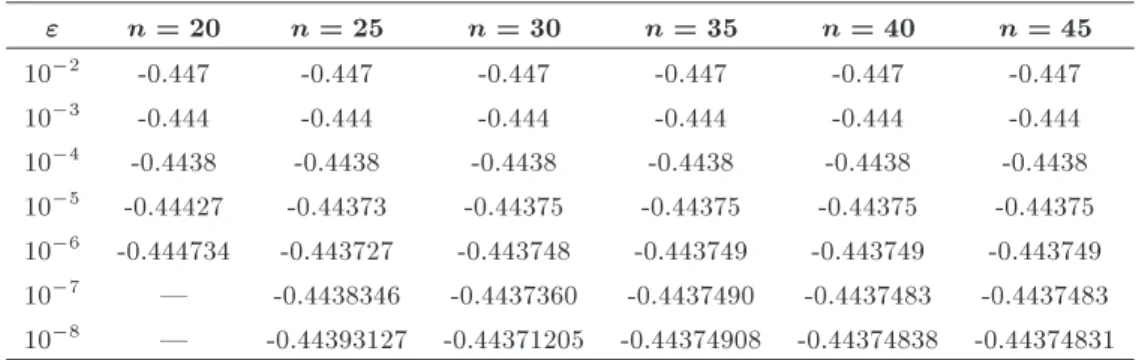
3.2. Numerical results for Sakiadis boundary layer problem
The convergence of solutions for the Sakiadis boundary layer problem is studied in Tables 4 and 5. It can be seen that when a small number of sampling points are used, the convergence and accuracy of the solutions are not very satisfactory for small values of ". For instance, when n = 20, accurate converged solutions can be achieved only for " 10 4. Note that the
solutions with n = 20 are not acceptable in accuracy when " 10 6. The convergence and accuracy of
the number of sampling points. In Table 6, the results are compared with the shooting results of Ref. [45]. A good agreement can be seen.
3.3. Numerical results for Falkner-Skan boundary layer problem
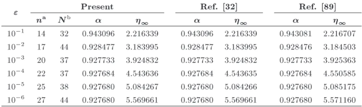
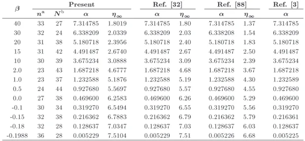
In Table 7, the results for wall shear stress and a truncated boundary are compared with those of [32,89]. The present results have closer agreement with the results of [32] than those of [89]. The results for dierent values of are given in Table 8. The results of [3,32,88] are also shown for comparison. An excellent agreement can be observed.
3.4. Numerical results for MHD Falkner-Skan boundary layer problem
The numerical results for dierent types of MHD Falkner-Skan boundary layer are tabulated in Tables 9-11. These results are calculated using n = 50 to
insure the stability, convergence and accuracy of the solutions.
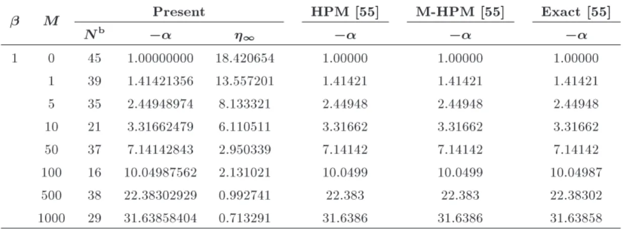
In Table 9, the present results are compared with the exact, shooting and AMD solution results of [28]. Comparing the results with those of analytical solutions, it is found that the present results are more accurate than the shooting and AMD solutions. It is interesting to note that the present results can match exact data up to 13 decimal digits. These results conrm the high accuracy and eciency of the proposed procedure for solving boundary layer problems dened on an innite domain. In Table 10, the present results are compared with those of [35]. It can be seen that the present results have closer agreement with the HAM solution results of [35] than those of other methods. In Table 11, some further comparisons are made with HPM solutions of [55]. A good agreement can be observed.
Table 6. Computed results for the Sakiadis equation (n = 45).
Present Shooting [45]
f() f0() f00() f() f0() f00()
0.0 0.00000000 1.00000000 0.44374831 0.00000000 1.0000000 0.44374733 0.5 0.44507728 0.78241753 0.41878277 0.44507720 0.7824172 0.41878160 1.0 0.78620198 0.58715319 0.35831281 0.78620150 0.5871525 0.35831140 5.0 1.57884695 0.02994984 0.02392277 1.57884400 0.0299497 0.02392260
6.17361 1.60163334 0.01168424 0.00939931 | | |
8.97449 1.61461504 0.00122014 0.00098550 | | |
10 1.61546582 0.00053288 0.00043052 1.61546300 0.0005329 0.00043052
11.81043 1.61597260 0.00012340 0.00009972 | | |
14.65716 1.61610999 0.00001236 0.00000999 | | |
15 1.61611369 0.00000936 0.00000758 1.61611200 0.0000094 0.00000758
17.50619 1.61612373 0.00000123 0.00000100 | | |
20 1.61612503 0.00000015 0.00000013 1.61611200 0.0000001 0.00000013
20.35562 1.61612508 0.00000011 0.00000010 | | |
23.20512 1.61612518 0.00000000 0.00000001 | | |
Table 7. Computed results for the truncated boundary 1 and the wall shear stress f00(0) = for the Falkner-Skan
equation (0= 1, = 1=2).
" Present Ref. [32] Ref. [89]
na Nb
1 1 1
10 1 14 32 0.943096 2.216339 0.943096 2.216339 0.943081 2.216707
10 2 17 44 0.928477 3.183995 0.928477 3.183995 0.928476 3.184503
10 3 20 37 0.927733 3.924832 0.927733 3.924832 0.927733 3.925363
10 4 22 37 0.927684 4.543636 0.927684 4.543635 0.927684 4.550585
10 5 25 38 0.927680 5.084267 0.927680 5.084266 0.927680 5.085175
10 6 27 44 0.927680 5.569661 0.927680 5.569661 0.927680 5.571160 a: Number of DQM sampling points;
Table 8. Computed results for the truncated boundary 1and the wall shear stress f00(0) = for the Falkner-Skan
equation (0= 1, " = 10 6).
Present Ref. [32] Ref. [88] Ref. [3]
na Nb
1 1 1
40 33 27 7.314785 1.8019 7.314785 1.80 7.314785 1.37 7.314785 30 32 24 6.338209 2.0339 6.338209 2.03 6.338208 1.54 6.338209 20 31 38 5.180718 2.3956 5.180718 2.40 5.180718 1.83 5.180718 15 31 42 4.491487 2.6740 4.491487 2.67 4.491487 2.50 4.491487 10 30 39 3.675234 3.0888 3.675234 3.09 3.675234 2.39 3.675234 2.0 23 43 1.687218 4.6777 1.687218 4.68 1.687218 3.67 1.687218 1.0 23 37 1.232588 5.1876 1.232588 5.19 1.232588 4.30 1.232589 0.5 24 44 0.927680 5.5697 0.927680 5.57 0.927680 4.55 0.927680 0.0 27 38 0.469600 6.2583 0.469600 6.26 0.469600 5.29 0.469600 -0.1 30 34 0.319270 6.5494 0.319270 6.55 0.319270 5.56 0.319270 -0.15 32 38 0.216362 6.7883 0.216362 6.79 0.216362 5.79 0.216361 -0.18 32 28 0.128637 7.0347 0.128637 7.03 0.128637 6.03 0.128637 -0.1988 36 28 0.005229 7.5104 0.005229 7.51 0.005226 6.68 0.005225
a: Number of DQM sampling points;b: Number of iterations.
Table 9. Computed results for the truncated boundary 1and f0(1) for the MHD Falkner-Skan equationa (n = 50,
" = 10 12).
fw M kp Present Exact [28] Shooting [28] AMD [28]
Nb f0(1)
1 f0(1) f0(1) f0(1)
0.1 0.5 5 35 0.2579991896208 20.601002 0.2579991896208 0.2580018814864 0.2579991264067 0.4 0.5 5 35 0.2189108749214 18.500132 0.2189108749214 0.2189120624529 0.2189108467711 0.7 0.5 5 49 0.1826835240527 16.036028 0.1826835240527 0.1826846008492 0.1826835145613 0.1 1.0 5 31 0.2156535254584 18.500101 0.2156535254584 0.2156547493061 0.2156535231532 0.1 1.5 5 59 0.1837961120799 16.410206 0.1837961120799 0.1837972387054 0.1837961119397 0.1 0.5 1 59 0.1955519507823 17.064271 0.1955519507823 0.1955532080746 0.1955519503997 0.1 0.5 1.5 28 0.2180983639145 19.011001 0.2180983639145 0.2180996387404 0.2180983610746 0.1 0.5 2 33 0.2310555387640 19.300032 0.2310555387640 0.2310569393893 0.2310555305671
a: f000() + f()f00() f0()2 (M + 1=kp)f0() = 0, f(0) = fw, f0(0) = 1, f0(1) = 1;b: Number of iterations.
Table 10. Computed results for the truncated boundary 1and the wall shear stress f00(0) = for the MHD
Falkner-Skan equationa (n = 50, " = 10 8).
M Present HAM [35] Crocco [35] Shooting [35]
Nb
1
4/3
1 37 1.71946568 5.590004 1.71947219 1.71076376 1.71946540 2 23 2.43949896 5.027111 2.43949870 2.43348047 2.43949833 5 30 5.19095980 3.391341 5.19095980 5.18824018 5.19095945 10 18 10.09677575 2.017002 10.09677575 10.09539387 10.09677545 50 25 50.01944084 0.458002 50.01944084 50.01916312 50.01944071 100 24 100.00972177 0.236502 100.00972177 100.00958289 100.00972170
-3
3 21 2.27338480 5.630001 2.27338419 2.26555724 2.27338836 4 24 3.48814584 4.561011 3.48814572 3.48374014 3.48814857 5 31 4.60075228 3.826141 4.60075228 4.59755490 4.60075494 10 22 9.80646300 2.094001 9.80646300 9.80502889 9.80646420 15 27 14.87167401 1.439103 14.87167401 14.87073502 14.87167484 20 10 19.90393626 1.100002 19.90393626 19.90323635 19.90393701 50 28 49.96165198 0.459013 49.96165198 49.96137386 49.96165233
Table 11. Computed results for the truncated boundary 1 and the wall shear stress f00(0) = for the MHD
Falkner-Skan equationa (n = 50, " = 10 8).
M Present HPM [55] M-HPM [55] Exact [55]
Nb
1
1 0 45 1.00000000 18.420654 1.00000 1.00000 1.00000
1 39 1.41421356 13.557201 1.41421 1.41421 1.41421
5 35 2.44948974 8.133321 2.44948 2.44948 2.44948
10 21 3.31662479 6.110511 3.31662 3.31662 3.31662
50 37 7.14142843 2.950339 7.14142 7.14142 7.14142
100 16 10.04987562 2.131021 10.0499 10.0499 10.04987
500 38 22.38302929 0.992741 22.383 22.383 22.38302
1000 29 31.63858404 0.713291 31.6386 31.6386 31.63858
a: f000() + f()f00() f0()2 Mf0() = 0, f(0) = 0, f0(0) = 1, f0(1) = 0; b: Number of iterations.
Table 12. Computed results for the function f() for the Jeery-Hamel equationa (Ha = 0, Re = 110, = 3).
Present HAM [71] Runge-Kutta [71]
n = 20 n = 25 n = 30
0.0 1.000000000000 1.000000000000 1.000000000000 1.0000000000 1.0000000000 0.1 0.979235706518 0.979235706523 0.979235706523 0.9792357062 0.9792357085 0.2 0.919265885575 0.919265885585 0.919265885585 0.9192658842 0.9192658898 0.3 0.826533612270 0.826533612283 0.826533612283 0.8265336102 0.8265336182 0.4 0.710221183224 0.710221183238 0.710221183238 0.7102211838 0.7102211890 0.5 0.580499458790 0.580499458804 0.580499458804 0.5804994700 0.5804994634 0.6 0.446935067029 0.446935067042 0.446935067042 0.4469350941 0.4469350697 0.7 0.317408427566 0.317408427577 0.317408427577 0.3174084545 0.3174084270 0.8 0.197641094520 0.197641094528 0.197641094528 0.1976410661 0.1976410889 0.9 0.091230421094 0.091230421098 0.091230421098 0.09123022879 0.0912304211 1.0 0.000000000000 0.000000000000 0.000000000000 -0.00000047 0.0000000000
a: See Eq. (12)
3.5. Numerical results for Jeery-Hamel boundary layer problem
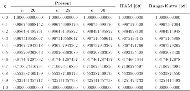
The numerical results for the Jeery-Hamel boundary layer problem with dierent values of , Re and Ha (dened in Eq. (12)) are shown in Tables 12-14. Tables 12 and 13 show the converging trend of the solutions, with respect to the number of sampling points. It is interesting to note that the present results may converge to 13 signicant gures for a small grid size of n = 25. From Tables 12 and 13, one also sees that the present results have closer agreement with Runge-Kutta solutions than the HAM solutions. In Table 14, the results are compared with VIM and Runge-Kutta solutions of [67]. It can be seen that the present results are in closer agreement with Runge-Kutta solutions than VIM solutions.
4. Formulation for unsteady two-dimensional boundary layer problems
Consider the unsteady two-dimensional boundary layer ow on a xed or moving at surface. The governing non-dimensional equation for boundary layer ow is given in Eq. (6). The boundary conditions are:
f(0; ) = c1;
f;(0; ) = c2;
f;(; ) = c3; (37)
where ci(i = 1; 2; 3) are constants. For the dierential
quadrature solution of Eq. (6), consider a grid of nm sampling points obtained by taking n and m points in
Table 13. Computed results for the function f() for the Jeery-Hamel equationa (Ha = 1000, Re = 50, = 5).
Present HAM [69] Runge-Kutta [69]
n = 20 n = 25 n = 30
0.0 1.000000000000 1.000000000000 1.000000000000 1.0000000000 1.0000000000 0.1 0.996756698152 0.996756698170 0.996756698170 0.9967570409 0.9967567004 0.2 0.986491485791 0.986491485822 0.986491485822 0.9864928100 0.9864914948 0.3 0.967516559607 0.967516559647 0.967516559647 0.9675193145 0.9675165808 0.4 0.936737943318 0.936737943362 0.936737943362 0.9367421766 0.9367379265 0.5 0.889208363043 0.889208363089 0.889208363089 0.8892135408 0.8892083429 0.6 0.817461287392 0.817461287437 0.817461287437 0.8174664644 0.8174612678 0.7 0.710623416794 0.710623416836 0.710623416836 0.7106275597 0.7106233991 0.8 0.553387469139 0.553387469173 0.553387469173 0.5533900638 0.5533874550 0.9 0.325141357717 0.325141357738 0.325141357738 0.3251423732 0.3251413493 1.0 0.000000000000 0.000000000000 0.000000000000 0.0000000000 0.0000000000
a: See Eq. (12).
Table 14. Computed results for the Jeery-Hamel equationa(Ha = 0, Re = 50, = 5, n = 25).
n Present VIM [67] Runge-Kutta [67]
f() f00() f() f00() f() f00()
0.0 1.00000000 -3.53941563 1.000000 -3.539369 1.000000 -3.539416 0.1 0.98243124 -3.38691089 0.982431 -3.386866 0.982431 -3.386911 0.2 0.93122596 -2.95779189 0.931227 -2.957753 0.931226 -2.957792 0.3 0.85061062 -2.32857378 0.850613 -2.328542 0.850611 -2.328574 0.4 0.74679080 -1.60178937 0.746794 -1.601767 0.746791 -1.601789 0.5 0.62694817 -0.87979398 0.626953 -0.879791 0.626948 -0.879794 0.6 0.49823445 -0.24394857 0.498241 -0.243994 0.498234 -0.243949 0.7 0.36696634 0.25560697 0.366974 0.255470 0.366966 0.255607 0.8 0.23812375 0.59970242 0.238131 0.599464 0.238124 0.599702 0.9 0.11515193 0.79300399 0.115157 0.792767 0.115152 0.793004 1.0 0.00000000 0.85436924 0.000000 0.854401 0.000000 0.854369
a: See Eq. (12).
0 and 0 , respectively. Satisfying
Eq. (6) at any sample point (i; j), one has:
f;(i; j) +12(1 j)if;(i; j)
+ jf(i; j)f;(i; j) f;2(i; j)
= j(1 j)f;(i; j);
i = 1; 2; ; n; j = 1; 2; ; m: (38) Now, using the quadrature rules, the quadrature analog of Eq. (38) is obtained as:
n
X
k=1
A(3)ikfkj+12(1 j) i n
X
k=1
A(2)ik fkj
+ j
2 4fij
n
X
k=1
A(2)ik fkj n
X
k=1
A(1)ikfkj
!23 5
= j(1 j) n
X
k=1 m
X
l=1
A(1)ikB(1)jl fkl;;
i = 1; 2; ; n; j = 1; 2; ; m: (39) Similarly, the quadrature analogs of boundary condi-tions are written as:
f1j= f(1; j) = c1; j = 1; 2; ; m;
(40) f;(1; j) =
n
X
k=1
A(1)1kfkj= c2; j = 1; 2; ; m;
(41) f;(n; j) =
n
X
k=1
A(1)nkfkj= c3; j = 1; 2; ; m:
(42) Using Eqs. (40)-(42) in Eq. (39), the boundary condi-tions can be invoked into the quadrature analog of the dierential equation. Then, an iterative scheme similar to that described in Section 3 can be used to obtain the truncated boundary and the solution of the unsteady two-dimensional boundary layer problem. Note that the unsteady two-dimensional boundary layer ow is also subjected to the following asymptotic boundary condition:
f;(; ) = 0 at (; ) = (1; ): (43)
Therefore, the convergence criteria for this case be-come:
f;(p; ) < " or jf;(n; )jp< "; (44)
where p is the iteration number, while n is the total number of sampling points in the -direction. The above criteria should be satised at 1; 2; ; m.
Therefore, to check the accuracy and convergence of the solutions, it is sucient to satisfy the following criteria:
max
1jmf;(
p; j) < " or
max
1jmjf;(n; j)jp< ": (45)
4.1. Numerical results
To demonstrate the eciency and accuracy of the proposed algorithm, application is made to a numerical
Table 15. Convergence of solutions for the wall shear stress f;(0; 0) = for the unsteady two-diensional
boundary layer problema(" = 10 3).
mb nc= 12 n = 15 n = 19 n = 24 n = 27 n = 30
2 -0.566 -0.564 -0.564 -0.564 -0.564 -0.564 3 -0.566 -0.564 -0.564 -0.564 -0.564 -0.564 4 -0.566 -0.564 -0.564 -0.564 -0.564 -0.564 5 -0.566 -0.564 -0.564 -0.564 -0.564 -0.564 6 -0.566 -0.564 -0.564 -0.564 -0.564 -0.564 7 -0.566 -0.564 -0.564 -0.564 -0.564 -0.564
a: See Eq. (6);
b: Number of DQM sampling points in -direction; c: Number of DQM sampling points in -direction.
example given by Liao [59]. A convergence study is rst made to determine proper values of n (number of sampling points in the -direction) and m (number of sampling points in the -direction) for discretization of the problem domain and for accurate solution of the boundary layer problem. The results for wall shear stresses (f;(0; 0) = ), with " = 10 3, are given
in Table 15. It can be seen that accurate converged results are achieved by the present method with n = 15 and m = 2. Note that m = 2 is the smallest number of sampling points that can be used in the proposed method for solving the present problem.
In Table 16, the results for wall shear stress and truncated boundary are given for various values of ". The analytic solutions of [59] are also shown for comparison purposes. It can be seen that the present results are matching with exact solutions to an excellent extent. These results conrm the high accuracy and eciency of the proposed procedure for solving unsteady boundary layer problems dened on an innite domain.
5. Formulation for unsteady three-dimensional boundary layer problems
Consider the unsteady three-dimensional boundary layer ow on a xed or moving at surface. The governing non-dimensional equation for boundary layer ow is given in Eqs. (8)-(10). The boundary conditions are:
f(0; ) = d1; f;(0; ) = d2; f;(; ) = d3;
(46)
Table 16. Computed results for the truncated boundary 1and the wall shear stress f;(0; 0) = for the
unsteady two-diensional boundary layer problema (m = 4).
" Present Exactd [59]
nb Nc
1
10 1 10 27 0.6 2.676 0.6
10 2 14 27 0.566 4.186 0.564
10 3 15 33 0.564 5.393 0.564
10 4 16 30 0.5642 6.393 0.5642
10 5 19 33 0.56419 7.265 0.56419
10 6 23 30 0.564190 8.048 0.564190
10 7 28 39 0.5641896 8.765 0.5641896
10 8 31 30 0.56418958 9.431 0.56418958
10 9 32 24 0.564189584 10.054 0.564189584
10 10 38 33 0.56418958355 10.631 0.56418958355 a: See Eq. (6);
b: Number of DQM sampling points in -direction; c: Number of iterations;
s(0; ) = d4; s;(0; ) = d5; s;(; ) = d6;
(47)
g(0; ) = d7; g(; ) = d8; (48)
where di(i = 1; ; 8) are constants. Satisfying
Eqs. (8)-(10) at any sample point (i; j), one has
(i = 1; 2; ; n, j = 1; 2; ; m):
f;(i; j) +12(1 j)if;(i; j) + j[(f(i; j)
+ s(i; j))f;(i; j) f;2(i; j)
Mf;(i; j)]=j(1 j) f;(i; j);
(49) s;(i; j) +12(1 j)is;(i; j) + j[(f(i; j)
+ s(i; j))s;(i; j) s2;(i; j)
Ms;(i; j)] = j(1 j)s;(i; j);
(50) g;(i; j) +12Pr(1 j)ig;(i; j)
+ Prj(f(i; j) + s(i; j))g;(i; j)
= Prj(1 j)g;(i; j): (51)
Now, using the quadrature rules, the quadrature analogs of Eqs. (49)-(51) are obtained as (i = 1; 2; ; n, j = 1; 2; ; m):
n
X
k=1
A(3)ikfkj+12(1 j)i n
X
k=1
A(2)ikfkj
+ j
"
(fij+ sij) n
X
k=1
A(2)ikfkj
n
X
k=1
A(1)ikfkj
!2
MXn
k=1
A(1)ikfkj
#
= j(1 j) n X k=1 m X l=1
A(1)ikBjl(1)fkl; (52)
n
X
k=1
A(3)ikskj+12(1 j)i n
X
k=1
A(2)ikskj
+ j
"
(fij+ sij) n
X
k=1
A(2)ikskj
n
X
k=1
A(1)ikskj
!2
MXn
k=1
A(1)ikskj
#
= j(1 j) n X k=1 m X l=1
A(1)ikB(1)jl skl; (53)
n
X
k=1
A(2)ikgkj+12Pr(1 j)i n
X
k=1
A(1)ikgkj
+ Prj(fij+ sij) n
X
k=1
A(1)ikgkj
= Prj(1 j) m
X
l=1
Bjl(1)gil: (54)
Similarly, the quadrature analogs of boundary condi-tions are written as (j = 1; 2; ; m).
f1j = f(1; j) = d1;
s1j= s(1; j) = d4;
g1j = g(1; j) = d7; (55)
f;(1; j) = n
X
k=1
A(1)1kfkj= d2;
s;(1; j) = n
X
k=1
A(1)1kskj = d5; (56)
f;(n; j) = n
X
k=1
A(1)nkfkj = d3;
s;(n; j) = n
X
k=1
A(1)nkskj= d6;
g;(n; j) = n
X
k=1
A(1)nkgkj= d8: (57)
Using Eqs. (55)-(57) in Eqs. (52)-(54), the boundary conditions can be invoked into the quadrature analog of the dierential equation. Then, a similar iterative scheme to that described in Section 4 can be used to obtain the truncated boundary and the solution of the unsteady three-dimensional boundary layer problem. 5.1. Numerical results
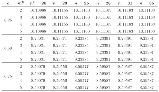
To demonstrate the eciency of the proposed algo-rithm, application is made to a numerical example given by Kumari and Nath [61]. Tables 17 and 18 present the convergence of solutions for the truncated boundary (1 ) and wall shear stress (f;(0; 1) = ),
Table 17. Convergence of solutions for the truncated boundary 1for the unsteady three-dimensional boundary layer
problema (M = 0, " = 10 5).
c mb nc= 20 n = 23 n = 25 n = 28 n = 31 n = 35
0.25
2 10.10968 10.11155 10.11160 10.11163 10.11163 10.11163 3 10.10968 10.11155 10.11160 10.11163 10.11163 10.11163 4 10.10968 10.11155 10.11160 10.11163 10.11163 10.11163 5 10.10968 10.11155 10.11160 10.11163 10.11163 10.11163
0.50
2 9.23031 9.23371 9.23384 9.23391 9.23391 9.23391 3 9.23031 9.23371 9.23384 9.23391 9.23391 9.23391 4 9.23031 9.23371 9.23384 9.23391 9.23391 9.23391 5 9.23031 9.23371 9.23384 9.23391 9.23391 9.23391
0.75
2 8.59079 8.59556 8.59577 8.59587 8.59587 8.59587 3 8.59079 8.59556 8.59577 8.59587 8.59587 8.59587 4 8.59079 8.59556 8.59577 8.59587 8.59587 8.59587 5 8.59079 8.59556 8.59577 8.59587 8.59587 8.59587
a: See Eqs. (8-11);
b: Number of DQM sampling points in -direction; c: Number of DQM sampling points in -direction.
Table 18. Convergence and comparison of solutions for the wall shear stress f;(0; 1) = for the unsteady
three-dimensional boundary layer problema (M = 0, " = 10 5).
c mb nc= 20 n = 23 n = 25 n = 28 n = 31 n = 35 HAM [61]
0.25
2 -1.04881 -1.04882 -1.04881 -1.04881 -1.04881 -1.04881
-1.04901 3 -1.04881 -1.04882 -1.04881 -1.04881 -1.04881 -1.04881
4 -1.04881 -1.04882 -1.04881 -1.04881 -1.04881 -1.04881 5 -1.04881 -1.04882 -1.04881 -1.04881 -1.04881 -1.04881
0.50
2 -1.09310 -1.09311 -1.09310 -1.09310 -1.09310 -1.09310
-1.09346 3 -1.09310 -1.09311 -1.09310 -1.09310 -1.09310 -1.09310
4 -1.09310 -1.09311 -1.09310 -1.09310 -1.09310 -1.09310 5 -1.09310 -1.09311 -1.09310 -1.09310 -1.09310 -1.09310
0.75
2 -1.13451 -1.13451 -1.13449 -1.13449 -1.13449 -1.13449
-1.13491 3 -1.13451 -1.13451 -1.13449 -1.13449 -1.13449 -1.13449
4 -1.13451 -1.13451 -1.13449 -1.13449 -1.13449 -1.13449 5 -1.13451 -1.13451 -1.13449 -1.13449 -1.13449 -1.13449
a: See Eqs. (8-11);
b: Number of DQM sampling points in -direction; c: Number of DQM sampling points in -direction.
with n and m, for three dierent values of c (see Eq. (11) for details). The HAM solutions of [61] are also included for comparison. It can be seen from Tables 17 and 18 that the present method can produce accurate converged solutions with n = 28 and m = 2.
In Table 19, the results for the truncated bound-ary, 1, and the wall shear stresses, f;(0; 1) = and
s;(0; 1) = , are compared with those of [61,90]. The
agreement between the results of the present method
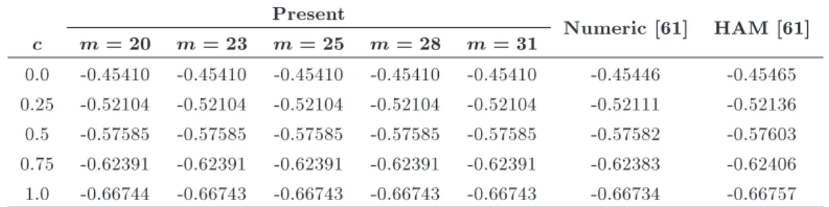
and those of [61,90] is excellent. In Table 20, the convergence and accuracy of solutions for g;(0; 1) =
are studied. The results are compared with numerical and HAM solutions of [61]. It can be seen that the results of the proposed formulation converge very quickly and agree well with those of [61]. These results conrm the correctness of the proposed procedure for solving unsteady three-dimensional boundary layer problems.
Table 19. Computed results for the truncated boundary 1and the wall shear stresses f;(0; 1) = , s;(0; 1) = for
the unsteady three-dimensional boundary layer problema (M = 0, " = 10 5, n = 31, m = 2).
Present Ref. [90] Ref. [61]
c Nb
1
0.0 41 1.00000 0.00000 11.51352 1.00000 0.00000 1.00000 0.00000 0.1 52 1.02026 0.06685 10.85150 1.02025 0.06684 1.02026 0.06685 0.2 42 1.03950 0.14874 10.33381 1.03949 0.14873 1.03950 0.14874 0.3 43 1.05796 0.24336 9.90832 1.05795 0.24335 1.05796 0.24336 0.4 48 1.07579 0.34921 9.54726 1.07578 0.34920 1.07580 0.34922 0.5 38 1.09310 0.46521 9.23391 1.09309 0.46520 1.09311 0.46521 0.6 55 1.10995 0.59053 8.95739 1.10994 0.59052 1.10995 0.59053 0.7 31 1.12640 0.72453 8.71021 1.12639 0.72453 1.12640 0.72455 0.8 54 1.14249 0.86669 8.48696 1.14248 0.86668 1.14250 0.86670 0.9 37 1.15826 1.01654 8.28361 1.15825 1.01653 1.15827 1.01655 1.0 46 1.17372 1.17372 8.09709 1.17372 1.17372 1.17374 1.17374
a: See Eqs. (8-11); b: Number of iterations.
Table 20. Convergence and comparison of solutions for g;(0; 1) = for the unsteady three-dimensional boundary layer
problema (M = 0, Pr = 0:7, " = 10 5, m = 2).
Present
Numeric [61] HAM [61] c m = 20 m = 23 m = 25 m = 28 m = 31
0.0 -0.45410 -0.45410 -0.45410 -0.45410 -0.45410 -0.45446 -0.45465 0.25 -0.52104 -0.52104 -0.52104 -0.52104 -0.52104 -0.52111 -0.52136 0.5 -0.57585 -0.57585 -0.57585 -0.57585 -0.57585 -0.57582 -0.57603 0.75 -0.62391 -0.62391 -0.62391 -0.62391 -0.62391 -0.62383 -0.62406 1.0 -0.66744 -0.66743 -0.66743 -0.66743 -0.66743 -0.66734 -0.66757
a: See Eqs. (8)-(11).
6. Solution of the Blasius boundary layer equation by reducing Blasius boundary value problem to a pair of initial-value problems
The Blasius boundary value problem can be reduced to a pair of initial value problems by means of a group of transformations [87]. The initial value problems are given by:
g000() +1
2g()g00() = 0; (58)
with initial conditions:
g(0) = g0(0) = 0; g00(0) = 1: (59)
And: f000() +1
2f()f00() = 0; (60)
with initial conditions:
f(0) = f0(0) = 0; f00(0) = [g0(1)] 3=2: (61)
These equations suggest a transformation of the form [87]:
g()= 1=3f(); =1=3;
=[g0(1)] 3=2: (62)
It is noted that g() is a bounded continuous function and, thus, g0(1) does exist. Let:
g0(1) = lim
!1g0() = L: (63)
It can be seen that if we solve Eq. (58) for g() and determine the magnitude of L, then we can obtain the solution of the Blasius equation from Eq. (60). 6.1. DQ analogs of resulting initial value
problems
The initial value problems given in Eqs. (58) and (60) can both be described by the following general initial
value problem: ...
F (t) +12F (t) F (t) = 0; (64)
with initial conditions:
F (0) = F0; _F(0) = _F0; F (0) = F0; (65)
where F0, _F0 and F0 are constants.
The third-order initial-value problem (Eq. (64)) can be converted into a set of rst-order initial-value problems as in the following:
8 > < > :
_x = y _y = z _z = 1
2xz
(66) with initial conditions:
x(0) = F0; y(0) = _F0; z(0) = F0: (67)
From the quadrature rule, Eq. (14), the rst-order derivative of functions x, y, and z can be expressed as:
_xi= m
X
j=1
A(1)ij xj; _yi= m
X
j=1
A(1)ij yj;
_zi= m
X
j=1
A(1)ij zj; i = 1; 2; ; m: (68)
Satisfying Eq. (66) at any sample time point, t = ti,
and substituting the quadrature rules given in Eq. (68) into results, gives:
8 > > > > > > > > > > > < > > > > > > > > > > > : m P j=1A (1) ij xj= yi
m
P
j=1A (1)
ij yj= zi i = 1; 2; ; m
m
P
j=1A (1)
ij zj = 12xizi
(69)
Applying the initial conditions (given in Eq. (67)) in Eq. (69) yields:
8 > > > > > > > > > > > < > > > > > > > > > > > : m P j=2A (1)
ij xj+ A(1)i1 F0= yi
m
P
j=2A (1)
ij yj+ A(1)i1 _F0= zi i = 2; 3; ; m m
P
j=2A (1)
ij zj+ A(1)i1 F0= 12xizi
(70)
Clearly, Eq. (70) is a nonlinear system of algebraic equations which can be solved using various iterative methods. In this study, we used the Newton-Raphson method to solve the system (70). Again we observed that only 3-5 iterations are sucient to achieve accu-rate solutions using the Newton-Raphson method. 6.2. A step-by-step DQ in time
For initial value problems, if the while time domain of interest is discretized simultaneously, many unknowns have to be solved simultaneously. As a result, it is more convenient to apply the DQM as a step-by-step time integration scheme to advance the solutions progressively over the time domain of interest [75-80]. In this technique, the time domain of interest is rst divided into a number of time elements. The DQM is then applied to each time element independently. The results at the end of each time element will then be used as initial conditions for the next time element (for more details, see [75-80]).
6.3. Numerical results and discussion
As mentioned earlier, we should rst determine the magnitude of L (dened in Eq. (63)). This parameter can be obtained using the solution of Eq. (58). To solve Eq. (58) using the scheme described in Section 6.2, we divide the time domain into nT equal length DQM time
elements with m sample time points (per DQM time element). The total number of sample time points and the average time step can be obtained as [75-79]:
Mtot= nT(m 1) + 1; (71)
t = T=(Mtot 1) = T=(nT(m 1)); (72)
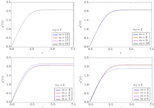
where T is the length of the time span. Figure 1 presents the variations of g0(t), with respect to t, for
dierent values of nT and m. It can be seen that
the DQM solutions converge rapidly by increasing nT
and/or m. It is clear that by increasing the number of time elements, a smaller number of sampling time points is required to achieve accurate solutions. Note that the DQM solution results at m time points are utilized to obtain the solutions at all the time domains via the Lagrange interpolation scheme. Thus, we are able to nd a continuous representation for function g0(t) using the Lagrange interpolation scheme.
It is interesting to note that the DQM yields converged and rather accurate solutions using only m = 3 time points. From Figure 1, it can also be seen that as t increases, g0(t) approaches a constant
value. This constant value is actually the magnitude of L. Note that in cases shown in Figure 1, the value of t is in the range 0 t 7:5. It is clear that in order to determine the magnitude of L(= g0(1)), it
is not necessary to solve the initial-value problem (58) in all the time domains, 0 t 1. For instance,
Figure 1. Convergence of DQM solutions with respect to the number of sample time points, m, and number of time elements, nT.
Table 21. Convergence of solutions for L = g0(t
1) (nT = 100).
m t1= 4:5 t1= 5:5 t1= 7:0 t1= 8:0 t1= 9:0 t1= 9:25 t1= 9:75 t1= 10:0
3 2.085 2.0854 2.0854 2.0854 2.0853 2.0853 2.0853 2.0853
4 2.085 2.0854 2.08541 2.08541 2.08541 2.08541 2.08541 2.08541
5 2.085 2.0854 2.08540917 2.08540917 2.08540917 2.08540917 2.08540917 2.08540917 6 2.085 2.0854 2.08540917 2.0854091764 2.0854091764 2.0854091764 2.0854091764 2.0854091764 7 2.085 2.0854 2.08540917 2.0854091764 2.085409176438 2.085409176438 2.085409176438 2.085409176438
as seen from Figure 1, one can solve the problem at the interval 0 t 7:5 to nd an approximation for L. In general, one can solve the problem in the time interval 0 t t1, where the magnitude of
t1 depends on the desired level of convergence and
accuracy. This can be clearly seen from the results shown in Table 21. These results are obtained using nT = 100 and dierent values of m. From Table 21,
one also sees that the accuracy of solutions for L will be improved by increasing the magnitude of t1. The best
results with shown tolerance values can be achieved when t1= 9. On the other hand, from Table 21, one
sees that the DQM cannot produce highly accurate solutions when the number of sampling points is too small.
The convergence of solutions for L = g0(9) is
studied in Table 22. It can be seen that the DQM results converge quickly without instability for an increase in nT and m. It can also be observed that
by increasing the number of sample time points (i.e.,
m), a smaller number of time elements (i.e., nT) are
required to obtain solutions with identical accuracies. Besides, when m is too small, the rate of convergence is too slow and very large values of nT are required
to achieve accurate solutions. In other words, the rate of convergence of the solutions is more sensitive to m than to nT. Thus, to obtain accurate solutions with
a reasonable time step size, one should rst choose the correct value of m and then increase nT to reach
the required level of accuracy. From Table 22, it is also observed that the magnitude of L is found to be converged up to 13 signicant gures for a small grid size of m = 8.
In Table 23, the DQM solutions are compared with those of the Runge-Kutta scheme for xed time step sizes. By comparing the DQM results with those of the Runge-Kutta scheme, one can conclude that the DQM can produce much better accuracy than the Runge-Kutta scheme using larger time step sizes. This illustrates the superiority of the DQM time
Table 22. Convergence of solutions for L = g0(9).
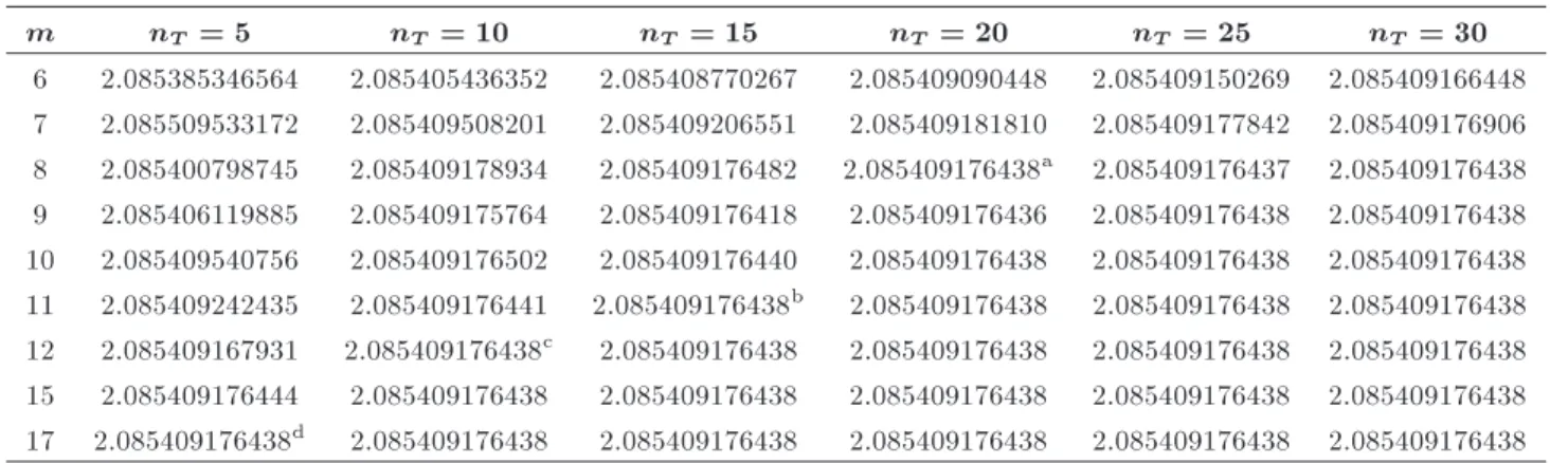
m nT = 5 nT = 10 nT = 15 nT = 20 nT = 25 nT = 30
6 2.085385346564 2.085405436352 2.085408770267 2.085409090448 2.085409150269 2.085409166448 7 2.085509533172 2.085409508201 2.085409206551 2.085409181810 2.085409177842 2.085409176906 8 2.085400798745 2.085409178934 2.085409176482 2.085409176438a 2.085409176437 2.085409176438
9 2.085406119885 2.085409175764 2.085409176418 2.085409176436 2.085409176438 2.085409176438 10 2.085409540756 2.085409176502 2.085409176440 2.085409176438 2.085409176438 2.085409176438 11 2.085409242435 2.085409176441 2.085409176438b 2.085409176438 2.085409176438 2.085409176438
12 2.085409167931 2.085409176438c 2.085409176438 2.085409176438 2.085409176438 2.085409176438
15 2.085409176444 2.085409176438 2.085409176438 2.085409176438 2.085409176438 2.085409176438 17 2.085409176438d 2.085409176438 2.085409176438 2.085409176438 2.085409176438 2.085409176438 a: t = 0:0642857;b: t = 0:06;c: t = 0:081818;d: t = 0:1125.
Table 23. Comparison of DQM solutions for L = g0(9) with those of Runge-Kutta scheme for a xed time step size.
Method t = 0:1125 t = 0:081818 t = 0:0642857 t = 0:06 t = 0:003 Present 2.085409176438 2.085409176438 2.085409176438 2.085409176438 2.085409176438 Runge-Kutta 2.085408947590 2.085409109185 2.085409150100 2.085409156321 2.085409176438
Table 24. Convergence of solutions for the wall shear stress f00(0) = for the Blasius equation (n T= 1).
m = 2 m = 3 m = 4 m = 5 m = 6 m = 7
0.3320573362152 0.3320573362152 0.3320573362152 0.3320573362152 0.3320573362152 0.3320573362152
integration method over the classical Runge-Kutta scheme.
Now, using the value of L = g0(1) = g0(9), we are
able to solve Eq. (60) with the boundary conditions given in Eq. (61). Note that Eq. (60) can be solved in any arbitrary domain of interest. Since we are interested in determining the wall shear stress, f00(0) =
, for the Blasius equation by the proposed method, we solved Eq. (60) in the interval [0; 0:1]. Table 24 demonstrates the convergence of solutions with respect to the number of sampling points. Only one DQM time element is used. An excellent convergence rate can be observed. It is interesting to note that the DQM can yield highly accurate solutions for the present problem using only m = 2 time points. Note that m = 2 is the smallest number of sample time points that can be used in the DQM for the solution of the present problem. The reason for this is that the present problem is a third-order nonlinear dierential equation and has three initial conditions at the initial time point. 7. Conclusion
In this paper, a general formulation based on the DQM is proposed for solving general boundary layer problems. At rst, a general formulation is pre-sented for solving Blasius, Sakiadis, Falkner-Skan, MHD Falkner-Skan and Jeery-Hamel boundary layer
problems. An iterative DQM is also presented for solv-ing unsteady, two-dimensional and three-dimensional, boundary layer problems. Finally, a simple scheme is proposed for solving the Blasius boundary layer equation. The eciency, accuracy and convergence of the proposed formulation for solving general boundary layer problems are investigated and analyzed. It is shown that the proposed iterative DQM can predict the behavior of the general boundary layer accurately. References
1. Schiliching, H., Boundary Layer Theory, 8th Ed., McGraw-Hill Inc (2004).
2. Howarth, L. \On the solution of the laminar boundary layer equations", Proc. Royal Soc. London, 164, pp. 547-579 (1938).
3. Asaithambi, A. \Solution of the Falkner-Skan equa-tion by recursive evaluaequa-tion of Taylor coecients", J. Comput. Appl. Math., 176, pp. 203-214 (2005). 4. Liao, S.J. \A kind of approximate solution technique
which does not depend upon small parameters, Part 2: an application in uid mechanics", Int. J. Non-Linear Mech., 32(5), pp. 815-822 (1997).
5. Liao, S.J. \An explicit, totally analytic solution of laminar viscous ow over a semi-innite at plate", Commun. Nonlinear Sci. Numer. Simulat., 3(2), pp. 53-57 (1998).
![Table 3 shows the computed wall shear stress and truncated boundary obtained by the proposed method and those reported in [32,88]](https://thumb-us.123doks.com/thumbv2/123dok_us/8394248.2230266/7.892.175.693.822.970/table-computed-stress-truncated-boundary-obtained-proposed-reported.webp)