Sharif University of Technology
Scientia IranicaTransactions E: Industrial Engineering www.scientiairanica.com
A multi-objective multi-state degraded system to
optimize maintenance/repair costs and system
availability
A. Salmasnia
a;, E. Ameri
b, A. Ghorbanian
b;1and H. Mokhtari
ca. Department of Industrial Engineering, Faculty of Engineering and Technology, University of Qom, Qom, Iran. b. Department of Industrial Engineering, Faculty of Engineering, Tarbiat Modares University, Tehran, Iran. c. Department of Industrial Engineering, Faculty of Engineering, University of Kashan, Kashan, Iran. Received 17 May 2015; received in revised form 12 December 2015; accepted 9 April 2016
KEYWORDS Multi-state system; Markov process; Multi-objective optimization; Preventive maintenance; Minimal repair; Desirability function.
Abstract.In this study, a multi-state degraded system is studied, where status of system is continuously degrading over time. As time progresses, system may either deteriorate gradually and go to lower performance state, or it may fail suddenly. If the system fails, some repairs are carried out to restore the system to the previous state. When the inspections reveal that the system has reached its last acceptable state, a PM is carried out to restore the system to the higher performance states. The goal is to nd the optimal PM level, so that the mean availability of the system is maximized and the total cost of the system is minimized. In this regard, Markov process is employed to represent dierent states of system. An integrated optimization approach is also suggested based on the desirability function of statistical approach. The suggested aggregation method is robust to the potential dependency between the total cost and the mean availability. It also ensures that both objective functions fall in decision-maker's acceptable region. In order to show the eciency of the proposed approach, a numerical example is presented and analyzed. © 2017 Sharif University of Technology. All rights reserved.
1. Introduction
A degraded system is an operating one whose status is degrading over time, and this degradation may aect its performance [1,2]. This phenomenon occurs in many real-world applications like transmission line networks, chemical processes, manufacturing industries, etc. In recent years, system availability has received extensive interest in many real-world systems such as com-puter [3] and communication systems [4],
transporta-1. Present address: Department of Industrial Engineering, Esfarayen University of Technology, North Khorasan, Iran. *. Corresponding author. Tel.: 02532103585;
E-mail addresses: [email protected] (A. Salmasnia); [email protected] (E. Ameri);
[email protected] (A. Ghorbanian); mokhtari [email protected] (H. Mokhtari)
tion systems [5], oil/gas production systems [6], etc. Most of studies considered two states for each system, so that the system was either working, or it com-pletely failed. This is called a binary-state system [7]. However, in many real-world cases, this binary-state assumption may not be sucient [8]. System may have more than two levels of performance varying from perfect functioning to complete failure. In other words, system may perform at various intermediate states between working perfectly and total failure [9,10]. The presence of degradation is a common situation in which a system should be considered to be a Multi-State Sys-tem (MSS). The gradual deterioration of sysSys-tem may be due to several reasons including the operating hours, the environmental conditions of the equipment, the failures of non-essential components, and the number of random shocks on the system. Basic concepts of
multi-stage systems have been introduced in [11-14]. Also, two pieces in literature review on multi-state systems can be found in [15,16]. A variety of approaches used in multi-state systems follow dierent perspectives which include:
1. The structure function approach in which Boolean models have been used for the multi-valued cases (e.g., in [12-14]);
2. The MonteCarlo simulation technique(e.g., in [17]);
3. The Markov process approach (e.g., in [18,19]);
4. The method of Universal Moment Generating Func-tion (UMGF) (e.g., see [20,21]).
One of the possible ways to improve a multi-state degraded system and to increase its availability is the use of Preventive Maintenance (PM). This will dra-matically reduce the costs of stopping the system [9]. Perfect PM aims to make the system as good as before starting to work, while imperfect PM may bring the system back to an intermediate state between the current state and the perfect functioning state [22]. In some papers like [23,24], a multi-state system with the state-dependent cost was investigated. In [25], a deteriorating repairable multi-state system with an imperfect policy was oered based on the number of system failures. In [26], a monotone process mainte-nance model for a multi-state system was developed. An analytical approach based on the failure number of the system was used to determine the optimal replacement policy. Soro et al. [27] suggested that if the system reaches the last acceptable degraded state, it is brought back to one of the states with higher ef-ciency employing preventive maintenance. Nourelfath et al. [28] formulated a joint redundancy and imperfect preventive maintenance planning optimization model for series-parallel multi-state degraded systems.
The majority of solution approaches used in the literature are single-objective approaches. In other words, most of the existing approaches concentrated only on maximizing system availability, and assumed
that there is no cost limitation [29-37], or consid-ered the cost limitation only as a constraint [38-40]. However, it is usually impossible for a single-objective approach to represent a practical problem truly. More-over, we can nd several reliability/availability ap-proaches to address dierent problems [41-46].
In this paper, a multi-state degraded system is considered. Even if the system deteriorates continu-ously, it is assumed that this process is done in a nite number of discrete states, and Markov chain is used to show the dierent states. It is also assumed that preventive maintenance can be performed in several dierent levels, varying from minor maintenance to major maintenance. A minor PM restores the system to the previous degraded state, while a major PM restores it to the \as good as new" state. The goal is to nd the optimal PM level, so that the mean availability of the system is maximized, and the total cost of the system is minimized during the useful lifetime of the system. The suggested integration approach includes the following features:
1. It is robust to the potential dependences between the total cost and the mean availability;
2. It aims to identify the settings of the decision vari-ables to maximize the degree of overall satisfaction with respect to total cost and mean availability. The remainder of the paper is organized as follows. In Section 2, the assumptions are presented and the multi-state degraded system under study is described. In Section 3, the availability and cost functions are repre-sented and a \minimum" operator for aggregating them is employed. In Section 4, an illustrative example is presented. Conclusions and some remarks are provided in Section 5.
2. Model description
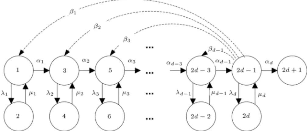
Initially, there is a system which is in its perfect functioning state (state 1). Over time as shown in Figure 1, two things may happen: the system may
either deteriorate gradually and go to the rst degraded state, or it may suddenly and randomly fail according to a Poisson process and go to a failed state. If the system fails, minimal repairs are carried out on it that restore the system to the previous state. When the system reaches the rst degraded state, it may either go to the second degraded state upon degradation, or may go to a failed state from which a minimal repair is performed. The same process will continue for all acceptable degraded states. When the system reaches an unacceptable state, it cannot satisfy the customers' demand in a required performance level and must be treated as a failure. If the inspection nds the system in its last acceptable state (state d), a PM is carried out to restore the system to one of the higher performance states. The described process is considered as a Markov process; the system-state transition diagram is shown in Figure 1.
2.1. Assumptions
The considered assumptions in the proposed model are as follows:
1. System can have dierent levels of degradation corresponding to discrete performance rates, which vary from perfect state to completely failed state;
2. System can randomly fail from any operational state, and then a minimal repair is done on it;
3. The repair time is negligible compared to the system's useful life. Therefore, it does not enter into the calculations;
4. All transition rates are constant with the exponen-tial distribution;
5. The current state of the system can be observed, and the time required for inspection is negligible. In other words, the inspection is carried out imme-diately.
2.2. System description
System-state transition can be described by the follow-ing notations and is illustrated in Figure 1:
: State (i), i = 1; ; n and n = 2d + m State (1): Perfect functioning;
State (2j 1), j = 2; ; d: The system satises the customer demand with an acceptable performance level;
State (2d+1): The system cannot satisfy the required demand after a degradation process and is in an unacceptable performance level;
State (2j), j = 1; ; d: The system encounters failure from an operational state and minimal repair must be carried out on it.
j: Failure rate or the transition rate
from state (2j 1) to the state (2j); j = 1; ; d;
j: Minimal repair rate or transition rate
from state (2j) to state (2j 1); j = 1; ; d;
j : Degradation rate or transition rate
from state (2j 1) to state (2j + 1); j = 1; ; d;
j : The preventive maintenance transition
rate from state (2d 1) to state (2j 1); j = 1; ; d 1.
3. The formulation of the problem
As mentioned before, the proposed method aims to simultaneously optimize the total cost and the mean availability of the system throughout its useful lifetime. Next, the method of calculating the total cost function and the mean availability function are described. 3.1. The total cost function
The total cost is the sum of the costs of preventive maintenance and repair during the system life cycle. The variable j is dened as a binary variable, so
that it is 1 if preventive maintenance is carried out from state (2d 1) to state (2j 1; j = 1; ; d 1); otherwise, it is zero. CPMj is the cost per unit time
incurred if a PM is performed from state (2d 1) to (2j 1; j = 1; ; d 1). pi is the probability of being
in the state i. It is assumed that the study period is given by the system life cycle T . Considering that T is large enough, there exists a steady-state distribution of state probabilities. In this case, the expected PM cost of system is a function of the decision variable, j, and
it is written as:
E(CPM) = T:p2d 1 d 1
X
j=1
(CPMj j): (1)
Since in state (2d 1), a PM is certainly performed. Also, we have Pd 1j=1 j = 1. In addition, CRj is the
cost per unit time incurred to repair system when it is in failed state (2j); j = 1; ; d. Therefore, the expected repair cost can be dened as follows:
E(CR) = TXd
j=1
CRj:p2j: (2)
Consequently, over the time interval [0; T ], the total cost of PM and repair is:
T C =T 2 4p2d 1
d 1
X
j=1
(CPMj j)+ d
X
j=1
CRj:p2j
3 5 : (3)
3.2. The availability function
In Figure 1, each state (2j 1; j = 1; ; d 1) is characterized by a performance rate (or capacity) explained by G2j 1, ranging from the best performance
rate G1 to the lowest one G2d 1 (G1 G2
G2d 1). It should be noted that the performance rate of
the failed states is zero (i.e., G2j = 0, j = 1; 2; ; d).
Finally, the performance rate of the unacceptable state (2d + 1) is less than customer demand. Since the performance rate at any time is a random variable, for the time interval [0; T ], the performance rate is a stochastic process. The probabilities associated with the various states at any time t 0 are given by the set P (t) = fp1(t); ; p2d+1(t)g, where:
pi(t) = Pr(G(t) = Gi); i = 1; ; 2d + 1: (4)
The system state acceptability depends on the relation between the system performance and the customer demand. This demand W (t) is usually a random variable that changes over time and can take a discrete value of the set W = fW1; ; W2d+1g. It is assumed
that demand is constant over time (W (t) = W ). As the system performance should exceed demand W , the acceptability function is dened as F (G(t); W ) = G(t) W [46]. According to our notations, it is assumed that G2d+1 < W G2d 1. Instantaneous availability,
A(t), is the probability that the system performance level at the moment t is greater than the customers' demand. In other word, system availability is the probability that the system is in one of acceptable states at time t.
A(t) = Pr(G(t) W ) =
d
X
j=1
p2j 1(t): (5)
Since every system enters the absorbing state as t becomes extremely large, the nal state probabilities are as follows:
lim
t!1p2d+1= 1; (6)
lim
t!1pj= 0 j = 1; ; 2d: (7)
According to the proposed Markov model in Figure 1, Chapman-Kolmogorov equations [27] are used to cal-culate pi(t). These equations are as follows:
dP1(t)
dt = (1+1)P1(t)+1P2(t)+1P2d 1(t) (8.1)1;
dP2j 1(t)
dt = (j+ j)P2j 1(t) + jP2j(t) + j 1P2j 3(t) + jP2d 1(t) j
for j = 2; ; d 1; (8.2)
dP2d 1(t)
dt = (j j+ d+ d)P2d 1(t) + dP2d(t) + d 1P2d 3(t)
for j corresponding to j= 1; (8.3)
dP2j(t)
dt = jP2j(t) + jP2j 1(t)
j = 1; 2; ; d; (8.4) dP2d+1(t)
dt = dP2d 1(t); (8.5) with the following initial values:
p1(t) = 1; p2(t) = p3(t) = = p2d+1(t) = 0: (9)
Also, for each t, 0 t T , we have:
2d+1X i=1
pi(t) = 1: (10)
Thus, Eqs. (8)-(10) are the constraints of optimization problem for a particular time of t. The objective function is maximizing the mean availability over the useful life of the system. The mean availability function of the system during the useful lifetime of the system is written as follows:
A =
T
R
t=0A(t)
T : (11)
3.3. The integration method
In order to do simultaneous optimization of the sys-tem cost and availability, an integrated optimization approach is suggested based on the desirability func-tion. The desirability function approach systematically transforms the objective function into a scale-free value called desirability. It assigns values between 0 and 1 to the possible values of objective function, in which desirability function gets 1 as the objective function gets its target value, and it will be zero when objective function lies outside its corresponding acceptable levels. Desirability function for system availability is shown in Eq. (12):
d A= 8 > < > :
A LA
UA LA LA A UA
0; A LA
(12)
where A is the obtained value for the system availability from Eq. (11), and UA can be set at the extreme value
of the system availability: UA= max A;
S.t. (Eqs. (8) to (10)): (13) UA, determined by Eq. (13), represents the maximum
region. LA is the lowest acceptable limit of system
availability which can be determined on the basis of the decision-maker's subjective judgment. In other words, the degree of satisfaction of a decision-maker with respect to system availability is maximized when
A equals its target value (UA) and decreases as A moves
away from UA. Finally, it will be zero when system
availability is less than LA.
Similarly, the desirability function of system cost is obtained from Eq. (14):
d(T C) = 8 > < > :
T C UT C
LT C UT C LT C T C UT C
0 T C UT C
(14)
where T C is the value obtained for the total cost function from Eq. (3), LT C is acquired by minimizing
the total cost function in a feasible region, and UT C is
asked from the decision-maker.
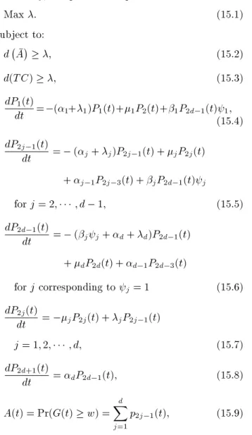
If a minimum operator is employed for aggre-gating the desirability functions of system cost and availability, an optimization problem can be stated as:
Max : (15.1)
Subject to:
d A ; (15.2)
d(T C) ; (15.3)
dP1(t)
dt = (1+1)P1(t)+1P2(t)+1P2d 1(t) (15.4)1;
dP2j 1(t)
dt = (j+ j)P2j 1(t) + jP2j(t) + j 1P2j 3(t) + jP2d 1(t) j
for j = 2; ; d 1; (15.5) dP2d 1(t)
dt = (j j+ d+ d)P2d 1(t) + dP2d(t) + d 1P2d 3(t)
for j corresponding to j= 1 (15.6)
dP2j(t)
dt = jP2j(t) + jP2j 1(t)
j = 1; 2; ; d; (15.7) dP2d+1(t)
dt = dP2d 1(t); (15.8)
A(t) = Pr(G(t) w) =Xd
j=1
p2j 1(t); (15.9)
2d+1X i=1
pi(t) = 1; (15.10)
pi(t) 0: (15.11)
This formulation aims to maximize the minimum sat-isfaction level of the decision-maker with respect to the system cost and the availability. It has several advantages over the existing methods.
Firstly, the majority of solution approaches in the literature assumed that there is no cost limitation or considered the cost limitation only as a constraint, whereas the proposed method optimizes total cost and system availability simultaneously.
Secondly, in contrast to other existing multi-objective approaches in literature, the suggested max-imin approach is robust to the potential dependency between the total cost and availability of the system. In other words, the correlation between the objective functions will not aect the optimization process. As a result, existing aggregation approaches used can lead to misleading results for this problem.
Thirdly, the suggested maximin approach creates a better balance between the objective functions in comparison with other existing aggregation methods. In other words, many aggregation methods may lead to a decision variable vector that the value of some of the objective functions may not be incredible in the decision-makers' view. In the proposed approach, rst, the acceptable range for each objective function is determined separately, and then it maximizes the overall satisfaction level within the ranges, such that the share of each objective function is properly reected in the optimization process.
4. Numerical example
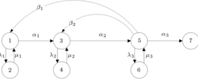
Consider a production system that has seven perfor-mance levels measured by hourly production rate, Gi.
These production rates are presented in Table 1. The customer demand, W , to be satised is 500 parts per hour. The Markov model of this multi-state system is illustrated in Figure 2.
According to the Markov model, there are two possible preventive maintenance actions. It is assumed that the transition rate of perfect PM (1) is equal
to 0.08, and the transition rate of imperfect PM (2)
is 0.02. The other used parameters are presented in Table 2.
The solution space of this problem has two cases which are:
Table 1. Hourly production rate for each state.
State i 1 2 3 4 5 6 7
Figure 2. System state transition diagram in a numerical example.
Table 2. Transition rates for the numerical example.
1 2 3 1 2 3 1 2 3
0.03 0.05 0.07 0.005 0.008 0.01 0.01 0.02 0.04 Table 3. The cost per hour incurred to repair system.
j 1 2 3
CRj 5.3 3.8 4.5
Table 4. Preventive maintenance cost incurred per hour.
j 1 2
CPMj 2.3 1.4 1= 1, 2= 0,
1= 0, 2= 1.
In order to evaluate the system availability, rst, Chapman-Kolmogorov equations are solved for the mentioned Markov model to obtain the probabilities Pi(t); (i = 1; ; 7) separately in both cases. Then,
the system availability at time t is calculated using A(t) = P1(t) + P3(t) + P5(t). Finally, assuming that
the useful life of the system is determined 80 hours, system availability ( A) and its corresponding desir-ability (d( A)) can be obtained by Eqs. (11) and (12), respectively.
The repair costs and the preventive maintenance costs are presented in Tables 3 and 4, respectively.
The expected repair and PM costs and the total cost will be calculated using Eqs. (1), (2), and (3), respectively. Then, the desirability function of the total cost and system availability will be achieved by assuming that the lower bound of acceptability for the system availability (LA) and the upper bound of
acceptability for the total cost (UT C) are 0.5 and 80,
respectively. After this step, the nal model can be written as follows:
Max ;
Subject to : d(A) ; d(T C) ; dP1(t)
dt = (1+ 1)P1(t) + 1P2(t) + 1P5(t) 1;
dP3(t)
dt = (2+ 2)P3(t) + 2P4(t) + 1P1(t) + 2P5(t) 2;
dP5(t)
dt = (j j+ 3+ 3)P5(t) + 3P6(t) + 2P5(t)
for j corresponding to j= 1;
dP2(t)
dt = 1P2(t) + 1P1(t); dP4(t)
dt = 2P4(t) + 2P3(t); dP6(t)
dt = 3P6(t) + 3P5(t); dP7(t)
dt = 3P5(t);
A(t) = P1(t) + P3(t) + P5(t); 7
X
i=1
pi(t) = 1;
pi(t) 0:
After solving the above mathematical programming us-ing MATLAB software package, the optimum solution is achieved as 1= 1, 2= 0.
Subsequently, this 1 = 0; 2 = 0 means that
during its useful life, whenever this system reaches the state 3, the perfect preventive maintenance is carried out; the system is restored to the perfect functioning state in this way.
5. Conclusion
This paper considered a multi-state degraded system in which status of system is considered to degrade over time, and this degradation may aect system performance. In other words, as time progresses, system may either deteriorate gradually and go to lower performance state, or it may suddenly and randomly fail according to a Poisson process called Poisson failure. If the system fails, minimal repairs are carried out to restore the system to its previous state. When the inspections showed that the system has reached its last acceptable state, a PM is carried out to restore the system to one of the higher performance states, varying from minor maintenance to major maintenance. A minor PM restores the system to the previous degraded state, while a major PM restores it to the \as good as new" state. To nd the optimal PM level, such that the mean availability of the system is maximized and
the total cost of the system is minimized, an integrated optimization approach is suggested based on the desir-ability function approach. The suggested aggregation method is robust to the potential dependency between the total cost and the mean availability. It also ensures that both objective functions fall in decision-maker's acceptable region.
As a direction for future research, the proposed model can be extended for a joint redundancy and imperfect preventive maintenance planning optimiza-tion problem for series-parallel multi-state degraded systems.
References
1. Jiang, Y., Chen, M. and Zhou, D. \Joint optimization of preventive maintenance and inventory policies for multi-unit systems subject to deteriorating spare part inventory", Journal of Manufacturing Systems, 35(1), pp. 191-205 (2015).
2. Yuan, W.Z. and Xu, G.Q. \Modelling of a deteriorat-ing system with repair satisfydeteriorat-ing general distribution", Applied Mathematics and Computation, 218(11), pp. 6340-6350 (2012).
3. Kumar, A., Saini, M., and Malik, S.C. \Performance analysis of a computer system with imperfect fault detection ofhHardware", Procedia Computer Science, 45(0), pp. 602-610 (2015).
4. Samad, M. \An ecient algorithm for simultaneously deducing MPs as well as cuts of a communication network", Microelectronics Reliability, 27(1), pp. 437-441 (1987).
5. Doulliez, P. and Jalnoulle, E. \Transportation network with random arc capacities", RAIRO, 3(1), pp. 45-60 (1972).
6. Aven, T. \Availability evaluation of oil/gas production and transportation systems", Reliability Engineering, 18(1), pp. 35-44 (1987).
7. Billinton, R. and Allan, R., Reliability of Power Systems, London, Pitman (1984).
8. Faghih-Roohi, S., Xie, M., Ming Ng, K. and Yam, R.C.M. \Dynamic availability assessment and optimal component design of multi-state weighted k-out-of-n systems", Reliability Ek-out-of-ngik-out-of-neerik-out-of-ng & System Safety, 123(0), pp. 57-62 (2014).
9. Sheu, S.-H., Chang, C.C., Chen, Y.L. and Zhang, Z.G. \Optimal preventive maintenance and repair policies for multi-state systems", Reliability Engineering & System Safety, 140(0), pp. 78-87 (2015)
10. Li, Y.F. and Peng, R. \Availability modeling and opti-mization of dynamic multi-state series-parallel systems with random reconguration", Reliability Engineering & System Safety, 127(0), pp. 47-57 (2014).
11. Murchland, J. \Fundamental concepts and relations for reliability analysis of multistate systems, reliability
and fault tree analysis", Theoretical and Applied As-pects of System Reliability, Philadelphia: SIAM, 3(1), pp. 581-618 (1975).
12. Barlow, S. and Wu, A. \Coherent systems with multi-state components", Mathematics of Operations Re-search, 3(1), pp. 275-281 (1978).
13. El-Neweihi, E., Proschan, F. and Sethuraman, J. \Multistate coherent systems", Journal of Applied Probability, 15(12), pp. 675-688 (1978).
14. Ross, S.M. \Multi valued state component systems", Annals of Probability, 7(2), pp. 379-83 (1979).
15. Lisnianski, A. and Levitin, G., Multi-State System Re-liability, Assessment, Optimization and Applications, Singapore, World Scientic Publishing Co. Pte. Ltd (2003).
16. Yingkui, G. and Jing, L. \Multi-state system re-liability: A new and systematic review", Procedia Engineering, 29(1), pp. 531-536 (2012).
17. Zio, E. and Podollini, L. \A Monte Carlo approach to the estimation of importance measures of multi-state components", Reliability and Maintainability Annual Symposium (RAMS), pp. 129-34 (2004).
18. Xue, J. and Yang, K. \Dynamic reliability analysis of coherent multi-state systems", IEEE Transactions on Reliability, 44(1), pp. 683-688 (1995).
19. Pham, H., Suprasad, A. and Misra, R. \Availability and mean life time prediction of multistage degraded system with partial repairs", Reliability Engineering & System Safety, 56(1), pp. 169-73 (1997).
20. Ushakov, I. \Universal generating function", Soviet Journal of Computing and System Science, 24(5), pp. 118-29 (1986).
21. Levitin, G., Universal Generating Functionin Reli-ability Analysis and Optimization, Berlin (Heidel-berg/New York): Springer-Verlag (2003).
22. Peng, R., Mo, H., Xie, M. and Levitin, G. \Optimal structure of multi-state systems with multi-fault cover-age", Reliability Engineering & System Safety, 119(2), pp. 18-25 (2013).
23. SU, C.-T. and Chang, C. \Minimization of the life cycle cost for a multi state system under periodic main-tenance", International Journal of Systems Science, 31(2), pp. 217-27 (2000).
24. Zhou, Y., Zhang, Z., Lin, T.R. and Ma, L. \Main-tenance optimisation of a multi-state series-parallel system considering economic dependence and state-dependent inspection intervals", Reliability Engineer-ing & System Safety, 111(1), pp. 248-259 (2013).
25. Zhang, Y., Yam, R. and Zuo, J. \Optimal replacement policy for a multistate repairable system", Journal of the Operational Research Society, 53(1), pp. 336-41 (2002).
26. Lam, Y. \A monotone process maintenance model for multistate system", Journal of Applied Probability, 42(1), pp. 1-14 (2005).
27. Soro, I., Nourelfath, M. and Ait-Kadi, D. \Per-formance evaluation of multi-state degraded systems with minimal repairs and imperfect preventive main-tenance", Reliability Engineering & System Safety, 95(2), pp. 65-69 (2010).
28. Nourelfath, M., Chatelet, E. and Nahas, N. \Joint redundancy and imperfect preventive maintenance optimization for series-parallel multi-state degraded systems", Reliability Engineering and System Safety, 103(1), pp. 51-60 (2012).
29. Aggarwal, K. \A simple method for reliability evalua-tion of a communicaevalua-tion system", IEEE Transacevalua-tions on Communications, 23(1), pp. 563-565 (1975).
30. Ke, W. and Wang, S. \Reliability evaluation for dis-tributed computing networks with imperfect nodes", IEEE Transactions on Reliability, 46(1), pp. 342-349 (1997).
31. Aven, T. \Some considerations on reliability theory and its applications", Reliabiality Engingineering & System Safety, 21(3), pp. 215-223 (1988).
32. Colbourn, C., The Combinatorics of Network Reliabil-ity, New York, Oxford University Press (1987).
33. Hoyland, A. and Rausand, M., System Reliability Theory: Models and Statistical Methods, New York, Wiley (1994).
34. Yeh, W. \A revised layered-network algorithm to search for all d-minpaths of a limited-ow acyclic network", IEEE Transactions on Reliability, 47(3), pp. 436-442 (1998).
35. Yeh, W. \Search for MC in modied networks", Computers & Operations Reseasrch, 28(2), pp. 177-184 (2001).
36. Yeh, W. \A simple algorithm to search for alld-MPs with unreliable nodes", Reliab. Engin. Sys. Safe, 73(1), pp. 49-54 (2001).
37. Yeh, W. \Search for all d-mincuts of a limited-ow network", Computers & Operations Reseasrch, 29(13), pp. 1843-1858 (2002).
38. Huang, H. \Fuzzy multi-objective optimization deci-sionmaking of reliability of series system", Microelec-tronics Reliability, 37(3), pp. 447-449 (1997).
39. Lin, J. \Evaluating the reliability of limited-ow net-works under the cost constraint", IIE Trans, 30(3), pp. 1175-1180 (1998).
40. Majety, S., Dawande, M. and Rajgopal, J. \Optimal reliability allocation with discrete cost-reliability data for components", Operations Research, 47(6), pp. 899-906 (1999).
41. Jahromi, E., Salmani. M.H. and Ghasemi, F. \A four-phase algorithm to improve reliability in series-parallel systems with redundancy allocation", Scientia Iranica, 21(3), pp. 1072-1082 (2014).
42. Amiri, M. and Ghasemi F. \A methodology for ana-lyzing the transient reliability of systems with identical comp onents and identical repairmen", Scientia Iran-ica, 14(2), pp. 72-77 (2007).
43. Fazlollahtabar, F. and Jalali, S.G. \Adapted Marko-vian model to control reliability assessment in multiple AGV", Scientia Iranica, 20(6), pp. 224-227 (2013).
44. Kianfar, F. \Optimal planning of equipment mainte-nance and replacement on a variable horizon", Scientia Iranica, 11(3), pp. 185-192 (2004).
45. Aven, T. \On performance measures for multistate monotone systems", Reliability Engineering & System Safety, 41(2), 259-266 (1993).
46. Mokhtari, H., Mozdgir, A. and Nakhai Kamal Abadi, I. \A reliability/availability approach to joint production and maintenance scheduling with multiple preventive maintenance services", International Journal of Pro-duction Research, 50(20), pp. 5906-5925 (2012).
Biographies
Ali Salmasnia is currently an Assistant Professor in University of Qom, Qom, Iran. His research interests include quality engineering, multi-response optimiza-tion, applied multivariate statistics, and multi-criterion decision making. He is the author or co-author of various papers published in Applied Soft Computing, Neurocomputing, IEEE Transactions on Engineering Management, International Journal of Advanced Man-ufacturing Technology, Applied Mathematical Mod-elling, Expert Systems with Applications, International Journal of Information Technology and Decision Mak-ing, and TOP.
Ehsan Ameri received his BS degree from the Islamic Azad University and his MS degree in Industrial Engineering from the Tarbiat Modares University in Iran. His current research interests include reliability, healthcare, and multi-criteria decision making. Ali Ghorbanian is a Lecturer in the department of Industrial Engineering in the Esfarayen University of Technology, North Khorasan, Iran. He holds master's degree of Industrial Engineering from the Tarbiat Modares University (TMU). His research interests are decision support systems, simulation, RSM, knowledge management, and process management.
Hadi Mokhtari is currently an Assistant Professor of Industrial Engineering in University of Kashan, Iran. His current research interests include the applications of operations research and articial intelligence tech-niques to the areas of project scheduling, production
scheduling, and supply chain management. He also published several papers in international journals such as Computers and Operations Research, International Journal of Production Research, Applied Soft
Com-puting, NeurocomCom-puting, International Journal of Ad-vanced Manufacturing Technology, IEEE Transactions on Engineering Management, and Expert Systems with Applications.