Vol. 9, No. 1, 2016, 64-83
ISSN 1307-5543 – www.ejpam.com
Application of Meshless Methods for Solving an Inverse Heat
Conduction Problem
Malihe Rostamian, Alimardan Shahrezaee
∗Department of Mathematics, Alzahra university, Vanak, Post Code 19834, Tehran, Iran.
Abstract. In this paper, we consider the inverse problem of determining the unknown temperature at
x=0 and section of initial condition att=0 in an inverse heat conduction problem (IHCP). Two new numerical methods are developed by using the solution of an auxiliary problem and heat polynomials as basis functions in presence of noisy data. Due to ill-posed IHCP, we use the Tikhonov regularization technique with the GCV scheme to solve the resulting matrix system of the basis function methods (BFM). Some numerical examples are presented to illustrate the strength of the methods.
2010 Mathematics Subject Classifications: 35R30, 35K05
Key Words and Phrases: IHCP, Basis function method, Tikhonov regularization method, meshless
method, GCV, Ill-conditioned, Heat polynomials, Auxiliary problem
1. Introduction
Inverse heat conduction problems (IHCPs) arise in many industrial and engineering appli-cations where heat transfer occurs. In remote sensing, oil exploration, nondestructive evalu-ation of material and determinevalu-ation of the earth’s interior structure. One of the applicevalu-ations may be the determination of the surface heat flux histories of reentering heat shield[32]. In some problems because of the physical situation at the surface that may be unsuitable for at-taching a sensor, some boundary conditions are unknown. For example, in a shuttle or missile reentering the earth’s atmosphere from space, the heat flux at the heated surface is needed [3].
Inverse problems are in nature ’unstable’ because the unknown solutions and parameters have to be determined from indirect observable data which contain measurement error. The major difficulty in establishing any numerical algorithm for approximating the solution is the ill-posedness of the problem and the ill-conditioning of the resulting discretized matrix. So far many different methods have been applied to solve IHCPs[2, 3, 6–8, 15, 18–20, 22, 24, 26, 28, 29, 31, 36, 37].
∗Corresponding author.
Email addresses:[email protected](M. Rostamian),[email protected](A.
Shahrezaee)
1.1. A Brief Review of Meshless Methods
The finite element method (FEM) and finite difference method (FDM) have been the dom-inant numerical methods in the solution of partial differential equations (PDEs) for several decades. Nevertheless, FEM and FDM possess some limitations in the solution of certain en-gineering problems:
(1) the generation of a well behaved mesh may be extremely time consuming procedure for complex geometry,
(2) large deformations produce highly distorted meshes,
(3) repeated remeshing with a moving discontinuity problem such as flame propagation is required,
(4) very slow convergence in high gradient regions is observed, etc.
In order to avoid these problems, an alternative approach, called mesh-less method, has been developed[17].
Meshless methods for the solution of PDEs can be grouped into two broad categories. One, as already mentioned, includes methods based on RBF interpolation. The second is based on the least squares technique. To this second class of methods belong element-free Galerkin methods[4], local Petrov-Galerkin technique[1], the finite point method[23]and the general finite difference method[21].
Radial basis functions (RBFs) were first applied to solve the partial differential equations in 1999 by Kansa[16]. This Kansa’s method is a technique based on direct collocation method. RBF performs[13, 27, 33]very well in interpolating highly irregular scattered data compared to many interpolating methods. These functions have been used in the boundary element method formulation such as the dual reciprocity method DRM[11], the method of fundamen-tal solution (MFS), the analog equation method (AEM) and the boundary knot method (BKM). These methods have been successfully applied to solve several non-linear problems[12].
In this paper two meshless approaches based on the use of the solution of an auxiliary problem and heat polynomials as radial basis functions (RBF) for determining the unknown temperature at x =0 and section of initial condition at t = 0 in an inverse heat conduction problem (IHCP), are devised. Since the basis functions are the general solution of considered heat equation, the approximation to the temperature distribution only needs to satisfy the boundary condition and the given measurement data. The proposed methods in this paper are based on the collocation method. Because of the collocation technique, these methods do not need to evaluate any integral. These approaches are different from most existing numerical algorithms in solving dynamical problems where the finite difference quotient will be used to discretize the time variable. Our methods are also feasible to handle various informal boundary conditions.
2. Mathematical Formulation of the Problem
In this work, we consider the following inverse problem:
Ut(x,t)−α2Ux x(x,t) =0; 0<x <1, 0<t<tma x, (1)
U(x, 0) =
¨
p(x); 0≤x <x∗,
f(x); x∗≤x≤1, (2)
U(0,t) =g(t); 0≤t≤tma x, (3)
U(1,t) =k(t); 0≤t≤tma x, (4) where 0<x∗<1,tma x is final time,αis the thermal diffusivity,pandkare known piecewise-continuous functions in their domain, while g and f are unknown functions. In order to determine f and glet us consider additional temperature measurements and heat flux given at a pointx =x∗, 0<x∗<1, as overspecified data:
U(x∗,t) =q(t); 0≤t≤tma x, (5)
Ux(x∗,t) =h(t); 0≤t≤tma x. (6) Some methods for determination of heat flux atx∗are discussed in[9, 10].
Problem (1)-(6) may be divided into two separate problems as shown in Figure 1.
←− ←− →
←− ←− →
←− ←− Known q(t) Known k(t) →
←− Unknown g(t) ←− Known h(t) →
←− ←− →
↓Known p(x) ↓Unknown f(x) →
x =0 x =x∗ x =1
Figure 1: Inverse heat conduction problem (1)-(6).
The first problem is:
Ut(x,t)−α2Ux x(x,t) =0; 0<x <x∗, 0<t<tma x, (7)
U(x, 0) =p(x); 0≤x ≤x∗, (8)
U(0,t) =g(t); 0≤t≤tma x, (9)
U(x∗,t) =q(t); 0≤t ≤tma x, (10)
Ux(x∗,t) =h(t); 0≤t≤tma x, (11) and the second problem is:
Ut(x,t)−α2Ux x(x,t) =0; 0<x∗<x <1, 0<t<tma x, (12)
U(1,t) =k(t); 0≤t≤tma x, (14)
U(x∗,t) =q(t); 0≤t≤tma x, (15)
Ux(x∗,t) =h(t); 0≤t≤tma x, (16) where gand f are unknowns.
Remark 1. For the problem (1)-(6), we can consider a conducting material that have 2 different layers and be described by the interval[0, 1]with the layers[0,x∗]and[x∗, 1]as following:
U(x,t) =
¨
U1(x,t); 0≤ x<x∗,
U2(x,t); x∗≤x ≤1.
In this case, we additionally require the continuity of the temperature and heat flux across two layers; i.e:
U1(x∗,t) =U2(x∗,t),
∂U1
∂x (x
∗,t) =∂U2
∂x (x
∗,t).
To solve the inverse problems (7)-(11) and (12)-(16), let us consider the following auxiliary problem
Ut(x,t)−α2Ux x(x,t) =0; 0<x <1, 0<t<tma x, (17)
U(x∗,t) =q(t); 0≤t ≤tma x, (18)
Ux(x∗,t) =h(t); 0≤t≤tma x, (19)
where q and h are known functions. Following the same method as in[30], we assume that a solution of (17)-(19) is represented as a power series[5],
U(x,t) = ∞
X
j=0
cj(t)(x−x∗)j,
where the coefficient cj(t)are to be determined. By substituting U into Ut−α2Ux x=0, we get:
cj+2=
c′j(t)
α2(j+1)(j+2), (j=0, 1, 2, . . .). (20)
Consequently, we obtain the following formal expression for U(x,t):
U(x,t) = ∞
X
j=0
[d jq(t)
d tj
(x−x∗)2j
α2j(2j)! +
djh(t)
d tj
(x−x∗)2j+1
The series in (21), however, may not be uniformly convergent. But, according to[5], if q and h are infinitely differentiable functions that are of the Holmgren class[5], i.e. they are infinitely differentiable functions defined on[0,tma x]that satisfy:
|q(j)(t)| ≤C1(2j)!x∗(−2j), |h(j)(t)| ≤C1(2j)!x∗(−2j), ∀j≥0,∀t ∈(0,tma x),
where C1>0is some constant. We should recall from[5]that the power series in (21) is uniformly convergent and U in (21) is a solution to (17)-(19).
The solution (21) exists and is unique but not always stable[5].
3. Heat Polynomials
We consider a solutionU of (1) in the form[5]:
U(x,t) =φ(x)ψ(t). (22)
Substituting (22) into (1) results:
U(x,t) =eλx+λ2α2t. (23) By expanding equation (23) into a Taylor’s series with respect toλ, we obtain:
U(x,t) = ∞
X
n=0
χn(x,t)λ
n
n!, (24)
whereχn are the heat polynomials which hold in equation (1). To computeχn, setting
eλx = ∞
X
n=0
anλn,
and
eλ2αt= ∞
X
n=0
bnλn,
where
an= x n
n!, n=0, 1, 2, . . . , and
bn=
(
α2dtd
d! ; n=2d,
0; n=2d+1, d=0, 1, . . . , it follows that:
eλx+λ2α2t= ∞
X
n=0
where
cn= n
X
j=0
bjan−j = [2n] X
d=0
α2dtd
d!
xn−2d
(n−2d)!. (26)
Here,[n2]denotes the largest integer less than or equal to n2. From equations (24), (25) and (26), it is clear that:
χn(x,t) =n!
[2n] X
d=0
α2dtd
d!
xn−2d
(n−2d)!. (27)
4. Numerical Procedures
Let∆ ={(xj,tj),j=1, . . . ,n+m+l}be a set of scattered nodes such that∆ = ∆1∪∆2∪∆3, where
∆1={(xj,tj), 0≤xj≤1, tj=0, j=1, . . . ,n},
∆2={(xj,tj), xj=x∗, 0≤tj≤1, j=n+1, . . . ,n+m},
∆3={(xj,tj), xj=x∗, 0≤tj≤1, j=n+m+1, . . . ,n+m+l},
and suppose thatΓ ={(xj,tj), j=1, . . . ,n+m+l}be also a set of scattered nodes such that Γ = Γ1∪∆2∪∆3, where
Γ1={(xj,tj), xj=1, 0≤tj≤1, j=1, . . . ,n}.
Then, discretizing of the boundary conditions (8), (10) and (11) in problem (7)-(11) at points ∆and boundary conditions (14)-(16) in problem (12)-(16) at pointsΓmay be considered as following:
U(xj, 0) =pj, j=1, 2, . . . ,n, (28)
U(x∗,tj−n) =qj−n, j=n+1,n+2, . . . ,n+m, (29)
Ux(x∗,tj−n−m) =hj−n−m, j=n+m+1, . . . ,n+m+l, (30) and
U(1,tj) =kj, j=1, 2, . . . ,n, (31)
U(x∗,tj−n) =qj−n, j=n+1,n+2, . . . ,n+m, (32)
Ux(x∗,tj−n−m) =hj−n−m, j=n+m+1, . . . ,n+m+l. (33) An approximate solution of problems (7)-(11) and (12)-(16) can be expressed as the following form[25]:
U∗(x,t) = n+Xm+l
j=1
λjϕ(x−xj,t−tj), (34)
where
T> tma x is a constant,λj are unknown constants which remain to be determined separately in problem (7)-(11) and (12)-(16) andUeis selected by the following two cases:
(BFM1) Ueis given by (21)[25].
(BFM2) Ue =Pny=1χn(x,t)where χn is given by (27), y is the number of heat polynomials and may be chosen arbitrary.
Using conditions (28)-(30) and (31)-(33), the values of theλj can be obtained by solving the following matrix equation:
Aλ=b, (36)
where
A=
ϕ(xr−xj,tr−tj)
ϕ(x∗−xj,ti−tj)
∂ ϕ
∂x(x
∗−x
j,ts−tj)
(n+m+l)×(n+m+l)
, (37)
bis an+m+l×1 vector which in problem (7)-(11) is:
b= pr qi hs
(n+m+l)×(1)
, (38)
and in problem (12)-(16) is
b= kr qi hs
(n+m+l)×(1)
, (39)
where r =1, 2, . . . ,n, i=n+1,n+2, . . . ,n+m,s=n+m+1,n+m+2, . . . ,n+m+l and
j=1, 2, . . . ,n+m+l.
Since the IHCP is ill-posed, matrix Ain equation (36) is ill-conditioned. Here, we use Tikhonov regularization method to solve equation (36)[14, 34]. The Tikhonov regularized solutionλµ for equation (36) is defined to be the solution to the following least square prob-lem:
min
λ {kAλ−bk
2+µ2kλk2}, (40)
where k · kdenotes the usual Euclidean norm and µ is called the regularization parameter. We use the GCV method to determine a suitable value ofµ.
Denote the regularized solution of equation (36) by λµ∗. The approximated solution Uµ∗
for problems (7)-(11) and (12)-(16) my be given as:
Uµ∗(x,t) = n+Xm+l
j=1
λµj∗ϕ(x−xj,t−tj), (41)
Finally the heat temperature at surfacex =0 and initial condition inx ∈[0,x∗]are given, respectively, by:
g(t) = n+Xm+l
j=1
and
f(x) = n+Xm+l
j=1
λµj∗ϕ(x−xj, 0−tj); 0<x∗≤x ≤1. (43)
5. Numerical Results and Discussion
In this section, we present and discuss the numerical results by employing BFM1 and BFM2 and compare them with each other. To test the accuracy of the approximate solution, we use the root mean square error (RMS) defined as[35]:
RM S(ψ(x)) =
v u u t 1
Nt
Nt
X
i=0
(ψE x ac t(xi)−ψAppr o x imat e(xi))2,
whereNt is total number of testing points in the domain of functionψ(x).
We apply the noisy data gei =gi+σ×r and(1)wheregiis the exact data and r and(1)is a random number between(0, 1)and the magnitudeσindicates the noise level of measurement data. The results are brought in tables and figures. All the computations are performed on the PC (pentium(R) 4 CPU 3.20 GHz).
Example 1. Consider the following problem:
Ut=αUx x; 0<x<1, 0<t <1, (44)
U(x, 0) =
¨1
2(x−
1
2)2; 0≤x<
1
2,
f(x); 12 ≤x ≤1, (45)
U(1,t) =1
4+2t; 0≤t≤1, (46)
U(1
2,t) =2t; 0≤t≤1, (47)
Ux(1
2,t) =2t; 0≤t≤1, (48)
whereα=2in0<x <12 andα=1in 12 <x <1. The exact solution of this problem is:
U(x,t) =
¨
U1(x,t) =12(x− 1
2)2+2t; 0≤x <
1
2,
U2(x,t) = (x−12)2+2t; 12 ≤x ≤1,
g(t) =1 8+2t,
f(x) =(x−1
2)
2.
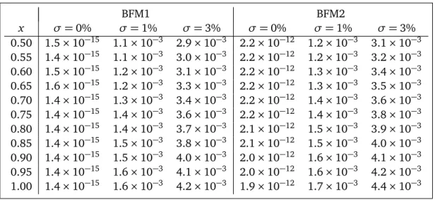
Tables 1 and 2 present the absolute errors|gN umer ic−gE x ac t|and|fN umer ic− fE x ac t|for various
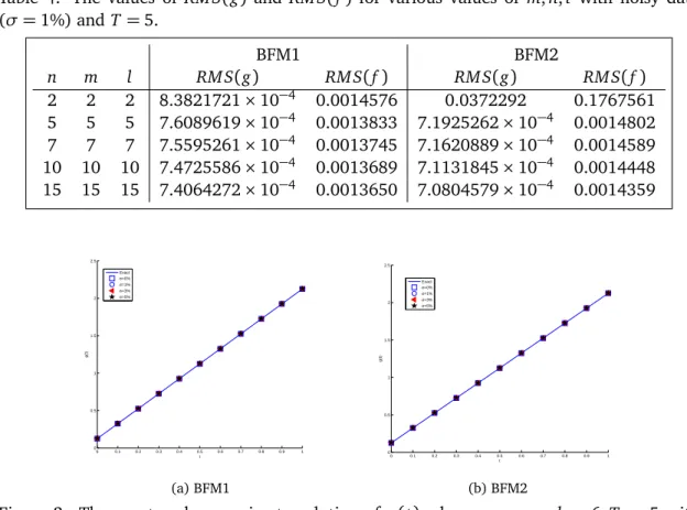
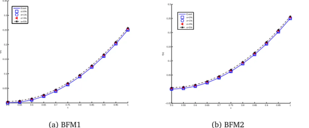
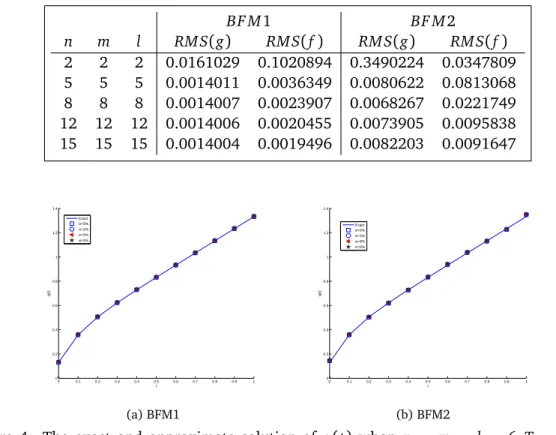
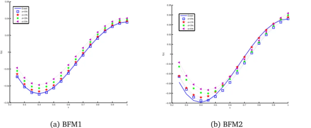
values of g(t) and f(x) for noiseless and noisy data (σ = 0%, 1%, 3%, 5%). From these Tables and these Figures, the numerical results are quite satisfactory. In Table 3 we present the errors RMS as a function of the parameter T with noisy data (σ = 1%). It can be seen from this Table that numerical results are not only stable with respect to parameter T , but also almost they maintain at the same level of accuracy over a wide rage of values T . Similar conclusions can be drawn from the results for Example 2 which are shown in Table 7. To see the effectiveness of the collocation points, we present the RM S(g)and RM S(f)with varying number of collocation points in Table 4. It is noted that the increase of the number of nodal points improve the accuracy of the numerical results. From all tables and figures we conclude that the approximate results of BFM1 for noiseless data are more accurate than BFM2.
Table 1: The absolute errors ofg(t)whenn=m=l =6,T=5 with noiseless and noisy data.
BFM1 BFM2
t σ=0% σ=1% σ=3% σ=0% σ=1% σ=3%
0.0 1.4×10⁻¹⁴ 9.3×10⁻⁴ 2.4×10⁻³ 1.7×10⁻⁹ 1.0×10⁻³ 2.6×10⁻³ 0.1 1.4×10⁻¹⁴ 8.9×10⁻⁴ 2.3×10⁻³ 1.9×10⁻⁹ 9.0×10⁻⁴ 2.3×10⁻³ 0.2 1.4×10⁻¹⁴ 8.5×10⁻⁴ 2.1×10⁻³ 1.6×10⁻⁹ 7.9×10⁻⁴ 2.0×10⁻³ 0.3 1.4×10⁻¹⁴ 8.1×10⁻⁴ 2.0×10⁻³ 1.8×10⁻⁹ 7.0×10⁻⁴ 1.8×10⁻³ 0.4 1.4×10⁻¹⁴ 7.7×10⁻⁴ 1.9×10⁻³ 1.5×10⁻⁹ 6.3×10⁻⁴ 1.6×10⁻³ 0.5 1.4×10⁻¹⁴ 7.3×10⁻⁴ 1.8×10⁻³ 8.4×10⁻¹⁰ 5.6×10⁻⁴ 1.5×10⁻³ 0.6 1.4×10⁻¹⁴ 6.9×10⁻⁴ 1.7×10⁻³ 1.4×10⁻⁹ 5.8×10⁻⁴ 1.4×10⁻³ 0.7 1.3×10⁻¹⁴ 6.5×10⁻⁴ 1.6×10⁻³ 7.5×10⁻¹⁰ 5.8×10⁻⁴ 1.4×10⁻³ 0.8 1.3×10⁻¹⁴ 6.1×10⁻⁴ 1.5×10⁻³ 0.9×10⁻¹¹ 5.9×10⁻⁴ 1.5×10⁻³ 0.9 1.3×10⁻¹⁴ 5.6×10⁻⁴ 1.4×10⁻³ 2.6×10⁻¹⁰ 6.4×10⁻⁴ 1.6×10⁻³ 1.0 1.3×10⁻¹⁴ 5.2×10⁻⁴ 1.3×10⁻³ 3.8×10⁻¹⁰ 7.1×10⁻⁴ 1.8×10⁻³
Table 2: The absolute errors of f(x)whenn=m=l=5,T=5 with noiseless and noisy data.
BFM1 BFM2
x σ=0% σ=1% σ=3% σ=0% σ=1% σ=3%
Table 3: The values ofRM S(g)andRM S(f)for various values ofT with noisy data (σ=1%) andn=m=l=5.
BFM1 BFM2
T RM S(g) RM S(f) RM S(g) RM S(f)
1.01 7.6084689×10⁻⁴ 0.0013829 7.1926508×10⁻⁴ 0.0014809 3.01 7.6060300×10⁻⁴ 0.0013832 7.1925926×10⁻⁴ 0.0014802 5 7.6089619×10⁻⁴ 0.0013833 7.1925262×10⁻⁴ 0.0014802 7 7.6095451×10⁻⁴ 0.0013828 7.1923964×10⁻⁴ 0.0014802 10 7.6081813×10⁻⁴ 0.0013829 7.1925280×10⁻⁴ 0.0014802 20 7.6078507×10⁻⁴ 0.0013834 7.1914739×10⁻⁴ 0.0014803
Table 4: The values of RM S(g) and RM S(f) for various values of m,n,l with noisy data (σ=1%) andT =5.
BFM1 BFM2
n m l RM S(g) RM S(f) RM S(g) RM S(f)
2 2 2 8.3821721×10⁻⁴ 0.0014576 0.0372292 0.1767561 5 5 5 7.6089619×10⁻⁴ 0.0013833 7.1925262×10⁻⁴ 0.0014802 7 7 7 7.5595261×10⁻⁴ 0.0013745 7.1620889×10⁻⁴ 0.0014589 10 10 10 7.4725586×10⁻⁴ 0.0013689 7.1131845×10⁻⁴ 0.0014448 15 15 15 7.4064272×10⁻⁴ 0.0013650 7.0804579×10⁻⁴ 0.0014359
0 0.1 0.2 0.3 0.4 0.5 0.6 0.7 0.8 0.9 1 0
0.5 1 1.5 2 2.5
t
g(t)
Exact σ=0% σ=1% σ=3% σ=5%
(a) BFM1
0 0.1 0.2 0.3 0.4 0.5 0.6 0.7 0.8 0.9 1 0
0.5 1 1.5 2 2.5
t
g(t)
Exact σ=0% σ=1% σ=3% σ=5%
(b) BFM2
0.5 0.55 0.6 0.65 0.7 0.75 0.8 0.85 0.9 0.95 1 0 0.05 0.1 0.15 0.2 0.25 0.3 0.35 x f(x) Exact σ=0% σ=1% σ=3% σ=5% (a) BFM1
0.5 0.55 0.6 0.65 0.7 0.75 0.8 0.85 0.9 0.95 1 −0.05 0 0.05 0.1 0.15 0.2 0.25 0.3 x f(x) Exact σ=0% σ=1% σ=3% σ=5% (b) BFM2
Figure 3: The exact and approximate solution of f(x) when n = m = l = 5,T = 5 with noiseless and noisy data.
Example 2. Let us consider the following problem:
Ut=Ux x; 0<x <1, 0<t<1, (49)
U(x, 0) =
(
3(1−x)2−1
6 +
2
π2cos(π(1−x)); 0≤x <
1
5,
f(x); 15 ≤x ≤1, (50)
U(1,t) =−1 6+t+
2
π2exp(−π
2t); 0≤t≤1, (51)
U(1 5,t) =
23 150+t+
2
π2cos(
4
5π)exp(−π
2t); 0≤t≤1, (52)
Ux(1
5,t) =− 4 5+
2
πsin(
4
5π)exp(−π
2t); 0≤t≤1, (53)
The exact solution of this problem is
U(x,t) =3(1−x)
2−1
6 +t+
2
π2cos(π(1−x))exp(−π
2t),
g(t) =1 3+t−
2
π2 exp(−π
2t),
f(x) =3(1−x)
2−1
6 +
2
π2 cos(π(1−x)).
Table 5: The absolute errors ofg(t)whenn=m=l =12,T=1.01 with noiseless and noisy data.
BFM1 BFM2
t σ=0% σ=1% σ=3% σ=0% σ=1% σ=3%
0.0 1.9×10⁻⁸ 1.7×10⁻³ 3.7×10⁻³ 1.3×10⁻² 1.4×10⁻² 1.6×10⁻² 0.1 6.7×10⁻⁹ 1.4×10⁻³ 3.1×10⁻³ 1.9×10⁻⁴ 1.5×10⁻³ 3.1×10⁻³ 0.2 2.1×10⁻⁹ 1.3×10⁻³ 2.9×10⁻³ 2.4×10⁻³ 1.0×10⁻³ 4.6×10⁻⁴ 0.3 5.4×10⁻¹⁰ 1.3×10⁻³ 2.8×10⁻³ 4.2×10⁻³ 2.8×10⁻³ 1.3×10⁻³ 0.4 2.7×10⁻¹¹ 1.3×10⁻³ 2.8×10⁻³ 2.9×10⁻³ 1.5×10⁻³ 9.6×10⁻⁵ 0.5 8.2×10⁻¹¹ 1.3×10⁻³ 2.8×10⁻³ 1.4×10⁻³ 2.7×10⁻³ 4.2×10⁻³ 0.6 4.1×10⁻¹¹ 1.3×10⁻³ 2.8×10⁻³ 5.2×10⁻³ 6.5×10⁻³ 8.0×10⁻³ 0.7 5.6×10⁻¹¹ 1.3×10⁻³ 2.8×10⁻³ 3.7×10⁻³ 5.1×10⁻³ 6.5×10⁻³ 0.8 1.7×10⁻¹⁰ 1.3×10⁻³ 2.8×10⁻³ 3.3×10⁻³ 2.0×10⁻³ 5.0×10⁻⁴ 0.9 3.0×10⁻¹⁰ 1.3×10⁻³ 2.8×10⁻³ 7.4×10⁻³ 6.0×10⁻³ 4.5×10⁻³ 1.0 4.1×10⁻¹⁰ 1.3×10⁻³ 2.8×10⁻³ 1.5×10⁻² 1.6×10⁻² 1.8×10⁻²
Table 6: The absolute errors of f(x)whenn=m=l=12,T=1.01 with noiseless and noisy data.
BFM1 BFM2
x σ=0% σ=1% σ=3% σ=0% σ=1% σ=3%
Table 7: The values ofRM S(g)andRM S(f)for various values ofT with noisy data (σ=1%) andn=m=l=12.
BFM1 BFM2
T RM S(g) RM S(f) RM S(g) RM S(f) 1.01 0.0014006 0.0020455 0.0075399 0.0095838
3 0.0087923 0.0187542 0.0059202 0.0087923 5 0.0526107 0.1159522 0.0111424 0.0096519 7 0.0526152 0.1159473 0.0108588 0.0122928 10 0.0526188 0.1159588 0.0103002 0.0129093 20 0.0526188 0.1159509 0.0082595 0.0217635
Table 8: The values of RM S(g) and RM S(f) for various values of m,n,l with noisy data (σ=1%) andT =1.01.
BF M1 BF M2
n m l RM S(g) RM S(f) RM S(g) RM S(f) 2 2 2 0.0161029 0.1020894 0.3490224 0.0347809 5 5 5 0.0014011 0.0036349 0.0080622 0.0813068 8 8 8 0.0014007 0.0023907 0.0068267 0.0221749 12 12 12 0.0014006 0.0020455 0.0073905 0.0095838 15 15 15 0.0014004 0.0019496 0.0082203 0.0091647
0 0.1 0.2 0.3 0.4 0.5 0.6 0.7 0.8 0.9 1 0
0.2 0.4 0.6 0.8 1 1.2 1.4
t
g(t)
Exact σ=0% σ=1% σ=3% σ=5%
(a) BFM1
0 0.1 0.2 0.3 0.4 0.5 0.6 0.7 0.8 0.9 1 0
0.2 0.4 0.6 0.8 1 1.2 1.4
t
g(t)
Exact σ=0% σ=1% σ=3% σ=5%
(b) BFM2
0.2 0.3 0.4 0.5 0.6 0.7 0.8 0.9 1 −0.06
−0.04 −0.02 0 0.02 0.04 0.06
x
f(x)
Exact σ=0% σ=1% σ=3% σ=5%
(a) BFM1
0.2 0.3 0.4 0.5 0.6 0.7 0.8 0.9 1 −0.05
−0.04 −0.03 −0.02 −0.01 0 0.01 0.02 0.03 0.04 0.05
x
f(x)
Exact σ=0% σ=1% σ=3% σ=5%
(b) BFM2
Figure 5: The exact and approximate solution of f(x) when n = m = l = 5,T = 5 with noiseless and noisy data.
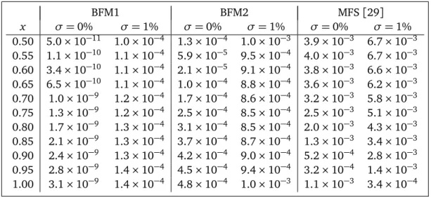
Example 3. Consider the following problem[29]:
Ut=Ux x; 0<x <1, 0<t<1, (54)
U(x, 0) =
¨
x2+sinx; 0≤x < 12,
f(x); 12 ≤x ≤1, (55)
U(1,t) =1+2t+exp(−t)sin 1; 0≤t ≤1, (56)
U(1 2,t) =
1
4+2t+exp(−t)sin( 1
2); 0≤t≤1, (57)
Ux( 1
2,t) =1+exp(−t)cos( 1
2); 0≤t≤1. (58)
The exact solution of this problem is
U(x,t) =x2+2t+exp(−t)sinx,
g(t) =2t,
f(x) =x2+sinx.
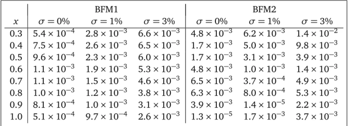
Table 9: The absolute error of g(t) whenn= m= l =5,T =1.01 with noiseless and noisy data.
BFM1 BFM2 MFS[29]
t σ=0% σ=1% σ=0% σ=1% σ=0% σ=1%
0.0 2.7×10⁻¹³ 8.0×10⁻⁴ 2.3×10⁻⁵ 1.0×10⁻³ 3.1×10⁻³ 2.0×10⁻³ 0.1 2.4×10⁻¹³ 7.4×10⁻⁴ 1.2×10⁻⁴ 6.4×10⁻⁴ 1.6×10⁻² 1.6×10⁻² 0.2 2.3×10⁻¹³ 6.8×10⁻⁴ 8.4×10⁻⁵ 4.9×10⁻⁴ 4.1×10⁻⁵ 4.2×10⁻⁴ 0.3 2.3×10⁻¹³ 6.4×10⁻⁴ 2.4×10⁻⁵ 4.8×10⁻⁴ 1.1×10⁻³ 1.6×10⁻³ 0.4 2.3×10⁻¹³ 5.9×10⁻⁴ 1.0×10⁻⁴ 5.2×10⁻⁴ 1.5×10⁻³ 1.0×10⁻³ 0.5 2.4×10⁻¹³ 5.6×10⁻⁴ 1.1×10⁻⁴ 5.5×10⁻⁴ 2.5×10⁻³ 2.0×10⁻³ 0.6 2.7×10⁻¹³ 5.3×10⁻⁴ 4.3×10⁻⁵ 5.6×10⁻⁴ 1.2×10⁻³ 6.7×10⁻⁴ 0.7 3.0×10⁻¹³ 5.0×10⁻⁴ 7.2×10⁻⁵ 5.2×10⁻⁴ 9.9×10⁻⁴ 1.5×10⁻³ 0.8 3.4×10⁻¹³ 4.9×10⁻⁴ 1.5×10⁻⁴ 4.8×10⁻⁴ 1.9×10⁻³ 2.4×10⁻³ 0.9 3.8×10⁻¹³ 4.7×10⁻⁴ 7.7×10⁻⁵ 4.8×10⁻⁴ 3.7×10⁻⁴ 1.4×10⁻⁴ 1.0 4.3×10⁻¹³ 4.6×10⁻⁴ 3.1×10⁻⁴ 6.0×10⁻⁴ 7.6×10⁻³ 7.1×10⁻³
Table 10: The absolute error of f(x)when n= m = l =5,T = 3 with noiseless and noisy data.
BFM1 BFM2 MFS[29]
x σ=0% σ=1% σ=0% σ=1% σ=0% σ=1%
0 1 2 3 4 5 6 7 0
1 2 3 4 5 6x 10
−3
σ
RMS(g)
BFM1 BFM2 MFS [17]
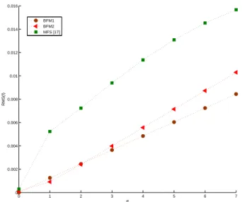
Figure 6: The values ofRM S(g)with various noise level andn=m=l=5,T=1.01.
0 1 2 3 4 5 6 7
0 0.002 0.004 0.006 0.008 0.01 0.012 0.014 0.016
σ
RMS(f)
BFM1 BFM2 MFS [17]
Figure 7: The values ofRM S(f)with various noise level andn=m=l=5,T =3.
6. Conclusion
by expanding the required approximate solutions using collocation based on basis function interpolation methods. Three numerical examples in the presence of various noise levels added in the input boundary data, have been solved. On the other hand, for all given examples the issue of numerical stability is discussed. It is shown that applying Tikhonov regularization method with GCV criterion for solving the final systems of equation (36), resulted in quite satisfactory findings that compare well with exact solutions.
References
[1] S. N. Atluri and T. Zhu. New meshless local petrov-galerkin (mlpg) approach in compu-tational mechanics. Computational Mechanics, 22:117–127, 1998.
[2] H. Azari, W. Allegretto, Y. Lin, and S. Zhang. Numerical procedures for recovering a time dependent coefficient in a parabolic differential equation. Dynamics of Continuous, Discrete and Impulsive Systems, Series B, Applications and Algorithms, 11:181–199, 2004. [3] J. V. Beck, B. Blackwell, and Ch. R. St. Clair Jr. Inverse Heat Conduction. John Wiley and Sons, A Wiley-Interscience Publication, Printed in the United States of America, 1985. [4] T. Belystchko, Y. Y. Liu, and L. Gu. Element-free galerkin methods. International Journal
for Numerical Methods in Engineering, 37:229–256, 1994.
[5] J. R. Cannon. The One Dimensional Heat Equation. Addison Wesley, Reading, MA, 1984. [6] C. L. Chang and M. Chang. Non-iteration estimation of thermal conductivity using finite volume method. International Communications in Heat and Mass Transfer, 33:1013– 1020, 2006.
[7] C. L. Chang and M. Chang. Inverse determination of thermal conductivity using semi-discretization method. Applied Mathematical modeling, 33:1644–1655, 2009.
[8] H. T. Chen and J. Y. Lin. Simultaneous estimations of temperature-dependent thermal conductivity and heat capacity.International Journal of Heat and Mass Transfer, 41:2237– 2244, 1998.
[9] P. Childs. Practical temperature measuremant. Butterworth-Heinemann, Linacre House, Jordan Hill, Oxford OX2 8DP 225 Wildwood Avenue, Woburn, MA 01801-2041 A Divi-sion of Read Educational and ProfesDivi-sional Publishing Ltd., 2001.
[10] P. Childs, J. Greenwood, and C. Long. Heat flux measurment techniques. Journal of mechanical engineering science, 213(7):655–677, 1999.
[12] M. Dehghan and R. Salehi. A meshless based numerical technique for traveling solitary wave solution of boussinesq equation. Applied Mathematical Modelling, 36:1939–1956, 2012.
[13] M. Dehghan and A. Shokri. A numerical method for solution of the two-dimensional sine-gordon equation using the radial basis functions. Mathematics and Computers in Simulation, 79:700–715, 2008.
[14] P. C. Hansen. Analysis of discrete ill-posed problems by means of the l-curve. SIAM Review, 34:561–580, 1992.
[15] C. H. Huang and C. Y. Huang. An inverse problem in estimating simultaneously the effective thermal conductivity and volumetric heat capacity of biological tissue. Applied mathematical modelling, 31:1785–1797, 2007.
[16] E. J. Kansa. Multiquadrics - a scattered data approximation scheme with applications to computational fluid-dynamics.Computers & Mathematics with Applications, 19:127–145, 1990.
[17] E. J. Kansa, R. C. Aldredge, and L. Ling. Numerical simulation of two-dimensional com-bustion using mesh-free methods.Engineering Analysis with Boundary Elements, 33:940– 950, 2009.
[18] S. Kim, M. C. Kim, and K. Y. Kim. Non-iterative estimation of temperature-dependent thermal conductivity without internal measurements. International Communications in Heat and Mass Transfer, 46:1801–1810, 2003.
[19] M. Lakestani and M. Dehghan. The use of chebyshev cardinal functions for the solution of a partial differential equation with an unknown time-dependent coefficient subject to an extra measurment.Journal of Computational and Applied Mathematics, 235:669–678, 2010.
[20] W. Liao, M. Dehghan, and A. Mohebbi. Direct numerical method for an inverse prob-lem of a parabolic partial differential equation. Journal of Computational and Applied Mathematics, 232:351–360, 2009.
[21] T. Liszka. An interpolation method for an irregular net of nodes. International Journal for Numerical Methods in Engineering, 20:1599–1612, 1984.
[22] C. S. Liu. One-step gps for the estimation of temperature-dependent thermal conductivity.
International Journal of Heat and Mass Transfer, 49:3084–3093, 2006.
[24] K. Parand and J. A. Rad. Kansa method for the solution of a parabolic equation with an unknown spacewise-dependent coefficient subject to an extra measurement. Computer Physics Communications, 184:582–595, 2013.
[25] R. Pourgholi and M. Rostamian. A numerical technique for solving ihcps using tikhonov regularization method. Applied Mathematical Modelling, 34:2102–2110, 2010.
[26] R. Pourgholi, M. Rostamian, and M. Emamjome. A numerical method for solving a non-linear inverse parabolic problem. Inverse problems in science and engineering, 18:1151– 1164, 2010.
[27] M. D. J. Powell. Radial basis functions for multivariable interpolation: a review, in: D.F. Griffiths, G.A. Watson (Eds.). Numerical Analysis. Longman scientific and Technical, Har-low, 1987.
[28] M. Shamsi and M. Dehghan. Recovering a time-dependent coefficient in a parabolic equation from overspecified boundary data using the pseudospectral legendre method.
Numerical Methods for Partial Differential Equations, 23:196–210, 2007.
[29] A. Shidfar, Z. Darooghehgimofrad, and M. Garshasbi. Note on using radial basis func-tion and tikhonov regularizafunc-tion method to solve an inverse heat conducfunc-tion problem.
Engineering Analysis with Boundary Elements, 33:1236–1238, 2009.
[30] A. Shidfar and R. Pougholi. Numerical approximation of solution of an inverse heat con-duction problem based on legendre polynomials. Applied Mathematics and Computation, 175:1366–1374, 2006.
[31] A. Shidfar, R. Pourgholi, and M. Ebrahimi. A numerical method for solving of a nonlinear inverse diffusion problem.Computers and Mathematics with Applications, 52:1021–1030, 2006.
[32] A. Shidfar and A. M. Shahrezaee. Existence, uniqueness and unstability results for an inverse heat conduction problem. International Journal of Applied Mathematics, 9:253– 258, 2002.
[33] M. Tatari and M. Dehghan. On the solution of the non-local parabolic partial differential equations via radial basis functions. Applied Mathematical Modelling, 33:1729–1738, 2009.
[34] A. N. Tikhonov and V. Y. Arsenin. On the Solution of Ill-Posed Problems. Wiley, New York, 1977.
[35] L. Yan, F. L. Yang, and C. L. Fu. A meshless method for solving an inverse spacewise-dependent heat source problem. Journal of computational physics, 228:123–136, 2009. [36] C. Y. Yang. Estimation of the temperature-dependent thermal conductivity in inverse