SYSPOINT: Unit of Measure for IT
Infrastructure Project Sizing
Srinivasa Raghavan
1and Veeraswamy Achanta
21President, Krea Corporation, IL, USA 2President, Rangasoft, IL, USA
What can be done to improve the success rate of IT infrastructure projects? The Standish group considers an IT project successful when it is completed on time and on budget, with all the features and functions originally specified. Thus, time, cost, and scope – the triple con-straint of project management is measured for success. The initial project estimation directly results in construct-ing the baseline for the two success parameters – time and cost. The traditional software estimation models uses lines of code and function points as sizing unit of measure. The IT infrastructure projects are significantly different from software development projects to use the software sizing techniques. This paper defines the con-cept of size for IT infrastructure projects. Specifically, the project size for IT infrastructure projects is measured in terms of the eight factors(server, workstation, printer, LAN, WAN, handheld, server applications, and client ap-plications), infrastructure related software components, and the complexities defined based on the physical and functional categories of those factors.
Keywords: information technology, project sizing,
in-frastructure, infrastructure project sizing, syspoint.
1. Introduction
In this competitive market environment, compa-nies try to differentiate their offerings through their IT infrastructure(Liu, 2002). For the
pur-pose of this study, IT infrastructure is defined as the hardware used to interconnect comput-ers and uscomput-ers and the software used to man-age the infrastructure. The advancement in the technology and the availability of cost effective hardware and networking options have encour-aged companies to expand and enrich their IT infrastructure. Liu (2002) suggest that the IT
infrastructure even though important, remains one of the poorly defined areas. The impor-tance is given more to IT software development
projects compared to that of the IT infrastructure projects. IT infrastructure projects are gener-ally considered subsets of large software devel-opment or package implementation initiatives. While this was true 15 years ago, the reduc-tion in the costs of hardware, innovareduc-tion of new devices, fast and affordable telecommunication medium has led to the increase in IT infrastruc-ture projects. The need for a reliable, consistent, and quantitative model to size and estimate ef-fort for infrastructure projects is evident. It is important to perform project sizing prior to es-timating the effort of a project(Peters, 1999).
The project estimation for these IT infrastruc-ture projects is performed primarily from a cost perspective. The size and effort of the IT infras-tructure projects are primarily estimated using qualitative techniques like expert judgment or analogy approach.
In the remainder of this paper, the literature of project sizing is discussed first. Next, the pa-per presents the methodology used to define a project size for IT infrastructure projects. The subsequent sections discuss the method to cal-culate IT infrastructure project size and the ad-vantages of such measure.
2. Concept of Project Sizing
It is important to perform project sizing prior to estimating the effort of a project(Peters, 1999).
The Standish group CHOAS report identifies inaccurate estimates as one of the key reasons of project failure(Johnson, Boucher, Connors,
and Robinson, 2001). Sizing is the key input
for all effort and costing models. Hence, de-termining the accurate size of a project is the requirement for precise cost and schedule esti-mation. The calculation of the project size can be extremely challenging at the early stages of the project. Project sizing determines how big a project is, based on some unit of measure. Prior to the mid 1970’s, qualitative techniques like expert judgment were used in determining the size of a project(Ferens, 1999). There was
no commonly accepted unit of measure to de-termine project size. The primary focus was given to software development projects. The programming languages used at that period of time influenced the development of sizing mod-els. The prevalent use of third generation lan-guages like COBOL during the 1970’s resulted in use of a sizing technique called “Lines of Code”. As the name indicates, the “lines of code” is based on the number of lines of code that will be written for a software project. This technique is still used as a sizing measure for various software costing models. The key ad-vantage of this method is its ease of use and understanding.
Even though this sizing technique is popular, it has a lot of drawbacks too. There is not a single standard definition on how to count the lines of code. As long as the counting tech-nique is consistent within an organization, it can be used to compare between projects and for other benchmarking purposes. However, comparing two projects between organizations using “Lines of Code” sizing technique requires several assumptions to be made. The major dis-advantage of this technique is its dependence
on the lines of code. Coding is just a phase of the software development life cycle. It does not account for the program complexity, vague requirements, bad design, and the choice of the life cycle model. It is also difficult to estimate the lines of code at the early stages of the project life cycle. If the requirement of the project is not detailed enough, sizing that project using this technique would be difficult and is as good as a speculation.
There are several variations of the technique like counting only the executable lines, counting executable lines plus data definitions, counting executable lines plus data definitions and com-ments(Jones, 1986). More variations are
possi-ble based on the type of the project. If a project is an enhancement of an existing project, the calculation of the lines of code can take vari-ations like, counting only new lines, counting new lines and changed lines, counting new lines, changed lines and reused lines. The “lines of code” technique depends on the programming language. If a project uses multiple program-ming languages, then the counting gets compli-cated. In spite of these drawbacks, “lines of code” is a widely used sizing technique even today!
The drawbacks of “lines of code” technique and its dependence on the programming language gave rise to another sizing technique called the “function point” technique. The concept of “function point” technique is to focus on the function requirements of the project to deter-mine the project size as against the lines of code. This idea was developed by Albrecht, an engineer at IBM (Dreger, 1989). The current
counting practices are published in a manual maintained by the organization called Interna-tional Function Point Users Group (IFPUG).
This manual defines “function point” technique as “measurement of software by quantifying the functionality the software provides to the user based primarily on the logical design” (
Func-tion point counting practices manual, 2000, p. 3). The basis of function point analysis is to
count function points that can be classified into five broad categories – External Input, External Output, Internal Logical File, External Interface File, and External Inquiry(Dreger, 1989).
the requirements stage of the project even with vague requirements. The “function point” tech-nique also has disadvantages. The rationale for the assigned weights in calculating unadjusted function points is not documented. Hence some organizations assign their own weights or some-times ignore the weights while calculating the unadjusted function points. It has been proved that not all of the five functional types are re-quired to be counted in calculating the unad-justed function points(Function point counting
practices manual, 2000). This technique is also
oriented towards the traditional data processing applications and cannot be applied to real time systems or scientific software (Abran, Maya,
and Desharnais, 1997).
Several extensions to the function point mea-sure were proposed in the past two decades. The most popular of these extensions is the fea-ture point analysis. It enables the function point measure to be applied to systems software and real-time applications. “Feature point” analy-sis includes a function type called algorithms in addition to the five function types identified by function point (Jones, 1986). Thus
appli-cations that have high algorithmic complexity such as real-time systems, process control ap-plications, embedded software applications etc, can be estimated using feature point analysis.
The object-oriented development methodology is significantly different such that traditional sizing measurements appear meaningless when applied. The popularity of the object-oriented design and development tools have resulted in a significant amount of research on estimating object-oriented projects.
One of the significant researches on estimat-ing object-oriented projects was performed by Chidamber and Kemerer. They have identified six different sizing metrics for object-oriented projects – Weighted methods per class, depth of inheritance tree, number of children, coupling between object classes, response for a class, and lack of cohesion in methods (Chidamber
and Kemerer, 1994).
The review of the software development sizing models highlights the fact that sizing is per-formed by counting the deliverables that can be quantified by the end users or the developers. In the case of “lines of code” technique, it was the size recognized by the developers. Function
point and feature point analyses focused pri-marily on the deliverables to the end user. The object point analysis focused on the number of objects that are recognized by the developers.
Extending this approach, the sizing of IT infras-tructure projects could be performed by count-ing the tangible hardware and network compo-nents of the projects that are recognized both by the end users and infrastructure technicians. The sizing technique for IT infrastructure pro-jects can be constructed similar to that of the function point analysis to include both the func-tion and the complexity of the project.
In this section, the concept of project sizing and the software development sizing models were discussed. The next section discusses the re-search methodology used to construct a sizing model for IT infrastructure projects.
3. Research Methodology
Qualitative research methodology was used to develop a sizing model for IT infrastructure projects. As a pilot, an expert interview was used to identify the factors that have an impact on the sizing of an infrastructure project. Fur-ther, a focus group of IT infrastructure experts were gathered to verify the sizing factors, de-velop a complexity matrix and the sizing model for IT infrastructure projects. The key research questions were:
What are the factors that affect the sizing of IT infrastructure projects?
What are the functional and physical char-acteristics of the factors identified?
What are the quantitative weights catego-rized by complexity for the characteristics of the factors identified?
The selection criteria for the expert interview was 10 years of IT infrastructure project man-agement (including project effort and cost
es-timation)experience and a minimum of 25 IT
infrastructure project management experience. The selection criterion was relaxed for the fo-cus group experts – 3 years of IT infrastructure project management experience and a minimum of 5 IT infrastructure project management ex-perience.
The need for participants was advertised using professional contacts, and the network of pro-fessional organizations. Each participant was required to submit their resume and participants were screened based on their willingness to participate, commitment to provide timely and active feedback and experience in the research topic. A total of eight experts provided their willingness to participate in the survey and six of them were selected to participate in the focus group. Two of them did not meet the time commitments required to participate in the focus group.
Expert A is a Senior Principal for an IT con-sulting firm with twelve years of IT infrastruc-ture project management experience and has managed $30 million worth of IT infrastruc-ture projects. This expert also is Cisco, Mi-crosoft, Novell, Comptia, and Citrix certified systems engineer. Expert B is a Principal for an IT consulting firm with seven years of IT infras-tructure project management experience and has managed about $20 million worth of IT infras-tructure projects. This expert is Cisco, UNIX, and Apple certified systems engineer. Expert C is a President of a consulting firm with 13 years of IT infrastructure project management experience. This expert has managed more than 75 network installation projects utilizing Mi-crosoft, Apple and Citrix technologies. Expert D is an IT Director for a Federal Government Agency. This expert has managed more than 10 government IT infrastructure projects utilizing mainframes, Microsoft and UNIX technologies. Expert E is a network architect in an IT con-sulting firm with ten years of IT infrastructure project management experience. This expert is Cisco, IBM, and Microsoft certified systems engineer. Expert F is an Engagement Mana-ger with 15 years of IT infrastructure project management experience. This expert has exten-sive experience in qualitative IT infrastructure project estimating.
Clear and open ended questions were presented to promote brain storming and also to chal-lenge the arguments in order to draw out the differences between the opinions and experi-ence. Proper analysis was performed to check if the data gathered are relevant to the topic of discussion. As mentioned earlier, one the big challenges of this technique was to main-tain the focus of the discussion. Conversations
easily tend to go in tangents and it was impor-tant to shift the focus to the objective. Good interpersonal skills, good analytical skills, non-judgmental approach, and flexibility of the re-searcher were key leadership traits that came in handy during the focus group research. These qualities resulted in the participants’ trust and increased the likelihood of open and interactive brain storming discussions.
The objective of the focus group was to find the answers to the three key research questions. An initial conference call was held to provide orien-tation to the experts about the research topic, the research questions, the concept of sizing, and the sizing methods used in the software deve-lopment area, the results of the pilot interview, and the timeframe. A PowerPoint presentation was developed for the purposes of this call, the research questions, and the results of the expert interview were sent to the focus group experts in advance. This helped to keep the discussion focused and work towards the common goal.
The focus group was conducted using an online method. An online discussion group system called “intranets.com” was used as the vehicle to launch this study. The focus group was con-ducted for a period of four weeks. The results of the research were validated by the experts during the fifth week.
The findings of the focus group research are presented in the following section. The experts identified the factors that impact the sizing of IT infrastructure projects, the functional and physical characteristics of those factors, cate-gorized them according to their complexity, and assigned weights by complexity. This structure was synonymous to that of the function point model. This research identified a new sizing unit of measure called syspoint.
4. Research Findings
use Low, Average, and High as the qualitative complexity grouping. Initially, the experts de-cided to keep both options open and try to cate-gorize the factors by very low, low, nominal, high, and very high categories. However, after preliminary categorizations, it was evident that the differences between the categories are neg-ligible and it made sense to use low, aver-age, and high as the categories. The experts identified eight key factors – server, server ap-plication, workstation, workstation apap-plication, printer, local area network, wide area network, and handheld application as factors that have an impact on IT infrastructure project sizing. There certainly can be several other general project-related factors that may have an impact on project sizing. Since this is one of the first researches carried out in this area of knowledge, it was decided to keep the scope simple and fo-cused.
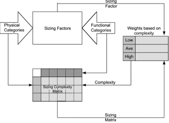
4.1. Sizing Process
The sizing process used by the focus group re-search is depicted in Figure 1. Each factor is defined and categorized by complexities using a matrix structure. The rows of the complexity matrix represent the physical categorization and
the columns of the complexity matrix represent logical or functional categorization.
After the complexity matrix was established for each factor, the experts then defined the sizing unit for each of the complexity within each fac-tor. The sizing unit for IT infrastructure projects was aptly named SYSPOINT. The experts de-cided to use the installation of a hub(
unman-aged switch)as one syspoint. Using the
instal-lation of one hub(or one syspoint)as the base,
the other complexities within and between the sizing factors were identified. Thus, the sys-point weights were carefully assigned by mak-ing sure that the weights assigned within and between the categories were proper and agreed to by all the experts.
The number of factors under each complexity is counted and multiplied by their corresponding syspoint weight to arrive at the total unadjusted syspoint for that factor. The total unadjusted syspoint for each factor is then summed to arrive at the total unadjusted syspoint for the project. An adjustment for the operating system is per-formed finally to arrive at an adjusted syspoint for the project. The server factor is explained in detail and to keep the paper focused and sim-ple, the sizing for other factors are grouped into tables.
4.2. Server Factors
For the purpose of this study, the experts defined servers as “A computer system in a network that is shared by multiple users. Servers come in all sizes from x86-based PCs to IBM mainframes”
(Techweb, 2003). The physical and functional
categories of the server factor are presented as rows and columns respectively in the following complexity matrix.
The single server represents categories where only one server is installed. The network load balancing servers implement a software scal-ing technology that spreads the client requests among servers that are connected to support a particular application (Techweb, 2003). In
defining the Cluster, one of the experts, re-ferred to the following definition from Tech-web(2003)“Using two or more computer
sys-tems that work together. It generally refers to multiple servers that are linked together in order to handle variable workloads or to pro-vide continued operation in the event one fails. Each computer may be a multiprocessor system itself. For example, a cluster of four computers, each with four CPUs, would provide a total of 16 CPUs processing simultaneously”.
The functional categories include new installa-tion, upgrade, and migration. New installation covers those projects when the installation of the server is performed from the scratch. Server up-grade refers to the upup-grade of different versions of the same operating system. For example, an upgrade of Windows 2000 from Windows NT is considered a server upgrade. Patch upgrades like Windows Service Packs are not covered by this sizing. They are considered normal main-tenance features and not installation projects. Server migration refers to the migration from one operating system to another operating sys-tem. For example, a migration from an UNIX Server to a LINUX Server or a migration from a Novell Server to a Windows 2000 Server is covered by this classification.
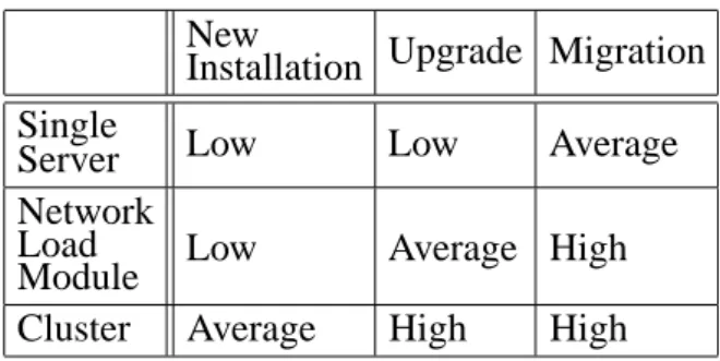
Table 1 represents the complexity matrix for the server factors. Using the physical tion as the row and the functional categoriza-tion as the column, the cells of the matrix are filled with Low, Average, or High values. For example, a single server migration is considered an average complex factor and a cluster server upgrade is considered a high complex factor.
New
Installation Upgrade Migration Single
Server Low Low Average
Network Load
Module Low Average High
Cluster Average High High
Table 1. Server Complexity Matrix.
Table 2 represents the weights (syspoint)
as-signed to each complexity of the server fac-tors. The weights are determined by the experts, based on their past experience. The weights are carefully assigned by taking into consideration their relationship within each sizing factor and between sizing factors. For example, the aver-age complexity server is considered about 1.7 times bigger than the low complexity server. Similarly, a low complexity server is consid-ered 3 times bigger than that of the average complexity workstation.
Unadjusted Syspoint Low complexity
servers 15
Average complexity
servers 25
High complexity
servers 40
Table 2. Server unadjusted Syspoint.
Based on the above definition of the low, aver-age, and high complexity servers, it is impor-tant that the total count of low, average, and high complexity servers is determined. Using the unadjusted syspoint from the table above, a total server unadjusted syspoint(λS) is then
calculated by multiplying the count of low, average, and high complexity servers with the corresponding unadjusted syspoint multiplier.
4.3. Workstation Factors
or stand alone to be used by a single user. Work-stations come in all sizes from dumb terminals to thin clients, to personal desktop computers, to Midrange and Mainframe Workstations”
(Techweb, 2003). The physical categories of
the workstation component were identified as dumb terminals, thin client-based terminals, and desktops or laptops. The functional categories were identified as new installation, cloned image, upgrade, and migration.
A dumb terminal was defined by an expert as a “display terminal without any processing abi-lity”. Dumb terminals are entirely dependent on the main server for processing functions. Even though the mainframe and mini computer ter-minals have some independent capabilities, they are still categorized as dumb terminals.
Thin clients are similar to dumb terminals, but with some capabilities. Thin clients do not per-form any application processing. They process only keyboard input and screen output and func-tion like an input/output terminal. The
applica-tion and funcapplica-tional processing are performed at the server level. However, the presentation and input mechanisms are performed at the terminal level(Techweb, 2003). Windows terminals and
the X-Window system are examples of this type of thin client. The focus group experts referred desktops as a personal computer or a Macintosh or a UNIX workstation that has individual pro-cessing capabilities and is able support multiple devices that could be shared or used as local devices.
The functional categories include new instal-lation, cloned image, upgrade, and migration. New installation covers those projects when the installation of the workstation is performed from the scratch. These categories are very si-milar to those of the server factors.
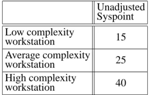
Table 3 represents the complexity matrix for the workstation factors. Using the physical catego-rization as the row and the functional categoriza-tion as the column, the cells of the matrix are
filled with Low, Average, or High values. The table below (Table 4) represents the weights
(syspoint) assigned to each complexity of the
workstation factors.
Unadjusted Syspoint Low complexity
workstation 15
Average complexity
workstation 25
High complexity
workstation 40
Table 4. Workstation unadjusted Syspoint.
Based on the above definition of the low, avera-ge, and high complexity workstations, it is im-portant that the total count of low, average, and high complexity workstations are determined. Using the unadjusted syspoint from the above table, a total workstation unadjusted syspoint
(λW)is then calculated by multiplying the count
of low, average, and high complexity worksta-tions with the corresponding unadjusted sys-point multiplier.
4.4. Printer Factors
The installation and configuration of the printer hardware is discussed in this section. The phy-sical categories of the printer component were identified as local printer, and network printer. The functional categories were identified as standard, duplex, and multi-function.
The local printer represents categories where the printers are connected directly to a port of a workstation. A local printer can also be shared with other computers through the workstation’s share capabilities. A network printer was de-fined by a focus group expert as follows: “When a printer is installed to be a network printer that can be shared with multiple workstations, it is
New installation Cloned Image Upgrade Migration
Dumb Terminal Low NA NA NA
Thin client Low Low Average Average
Desktops/Laptops Average Avg High High
called a network printer”. If a local printer is set up to be shared with other users, it should not be counted as network printer; it is still a local printer.
The functional categories include standard in-stallation, duplex, and multi-function. Stan-dard installation covers those projects with the installation of the printer with the default basic features that arrive with the printer. The duplex function refers to the back to back printing capa-bility of a printer. This requires additional con-figuration and installation of additional units. The multi-function capability refers to the in-stallation and configuration of devices that pro-vide features like copier, fax, and/or scanner in
the printer unit.
Standard Duplex Multifunction
Local Low Low Average
Network Low Average High
Table 5. Printer Complexity Matrix.
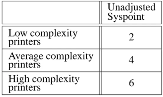
Table 5 represents the complexity matrix for the printer factors. Using the physical categoriza-tion as the row and the funccategoriza-tional categorizacategoriza-tion as the column, the cells of the matrix are filled with Low, Average, or High values. The table below (Table 6) represents the weights (
sys-point)assigned to each complexity of the server
factors.
Unadjusted Syspoint
Low complexity
printers 2
Average complexity
printers 4
High complexity
printers 6
Table 6. Printer unadjusted Syspoint.
Based on the above definition of the low, ave-rage, and high complexity printers, it is im-portant that the total count of low, average, and high complexity printers are determined. Using the unadjusted syspoint from the table above, a total printer unadjusted syspoint(λP)is
then calculated by multiplying the count of low, average, and high complexity printers with the corresponding unadjusted syspoint multiplier.
4.5. Local Area Network Factors
Local area network(LAN)is a data
communi-cation network that serves users within a con-fined area – mostly a building or even a small area within the building. The network would generally encompass servers, workstations, prin-ters, a network operating system and a commu-nication link (Techweb, 2003). The physical
categories of the local area network compo-nent were identified as “hubs” or unmanaged switches, managed switch without a VLAN, wireless VLAN, and managed switches with a VLAN. The functional categories were identi-fied as new direct connection, routing, limited access, and firewall.
Techweb (2003) defines a hub as, “a central
connecting device in a network that joins com-munication lines together in a star configura-tion”. There are two types of hubs – active and passive. Passive hubs are just connecting hubs and add nothing to the data that are passed through them. Active hubs are multi-port re-generators that can regenerate the data bits to maintain the strong signal and can include some intelligence. An unmanaged switch is a net-work switch that does not support any statistics or management-related queries.
Managed Switch is a network switch that has the intelligence built into the firmware. These switches can respond to statistical and manage-ment queries and typically would require addi-tional configuration for management and moni-toring purposes.
Wireless local area networks transmit the data through unlicensed frequency such as 2.4 GHz band. The wireless local area network does not require lining up of devices like the infra red transmission. This typically requires installa-tion of an access point(or a base station)that
is physically connected to the network. This base unit can transmit signals to multiple wire-less network cards using the radio frequency over a limited area, penetrating walls and other non-metal barriers.
Virtual local area network (VLAN) is a
cables. One of the focus group experts defined its function as – “It combines user stations and network devices into a single unit regardless of the physical LAN segment they are attached to and allows traffic to flow more efficiently within populations of mutual interest” (
Tech-web, 2003).
The functional categories include direct con-nection, router, limited access and firewall. The direct connection refers to the simple plug-in connectivity to the router or the modem. The router refers to the presence of a device in the network to forward data packets from one local area network to another. The routing functional category represents simple routing entries with-out any customization.
The limited access function represents the cus-tomization of the routing tables and routing pro-tocols that are read by the routers to translate the network address in each transmitted frame and make a decision on how to send it based on the most expedient route – based on parameters like traffic load, line costs, speed, and bad lines
(Techweb, 2003).
The firewall is a mechanism for implementing security policies designed to keep a network secure from intruders. Firewalls installed to protect entire networks are typically implemen-ted in hardware; however, software firewalls are also available to protect networks from attack
(Techweb, 2003).
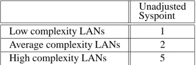
Table 7 represents the complexity matrix for the LAN factors. Using the physical categorization as the row and the functional categorization as the column, the cells of the matrix are filled with Low, Average, or High values. Table 8 repre-sents the weights (syspoint) assigned to each
complexity of the local area network factors.
Based on the above definition of the low, ave-rage, and high complexity LANs, it is impor-tant that the total count of low, average, and high complexity servers is determined. Using
Unadjusted Syspoint
Low complexity LANs 1
Average complexity LANs 2
High complexity LANs 5
Table 8. LAN unadjusted Syspoint.
the unadjusted syspoint from the table above, a total LAN unadjusted syspoint(λLAN) is then
calculated by multiplying the count of low, ave-rage, and high complexity printers with the cor-responding unadjusted syspoint multiplier.
4.6. Wide Area Network Factors
For the purpose of this study, the experts defined Wide area networks as “a communications net-work that covers a wide geographic area, such as state or country. A wide area network(WAN)
generally covers a wide geographic area”(
Tech-web, 2003). Physical categories of the WAN
component were identified as cable modems, ISDN/Frame relay, DS3/OC and wireless wide
area networks. The functional categories were identified as direct connectivity, router, limited access and firewall.
A cable modem is a hardware used to con-nect a computer to a cable television service that provides internet access. Cable modems have become a popular choice of wide area net-work at small companies and for home netnet-work setups. They provide high bandwidth network connectivity between the user’s computer and the internet service provider. Cable modems link to the computer via Ethernet, which makes the service online all the time.
Integrated services digital network (ISDN) is
an international telecommunication standard for providing a digital service from the customer’s premises to the dial-up network (Techweb,
2003). Frame relay is a high speed packet
Direct Routing Limited Access Fire-wall
Hubs/Unmanaged Switch Low N/A N/A N/A
Managed Switch without VLAN Low Average High High
Wireless LAN Avg Average High High
switching protocol and it has become a popu-lar choice for LAN to LAN connections across remote distances.
A focus group expert defined DS3/OC as
fol-lows: “Digital Signal (DS3)is a classification
of digital circuits. The DS technically refers to the rate and format of the signal, while the T designation refers to the equipment provid-ing the signals. In practice, “DS” and “T” are used synonymously; for example, DS1 and T1, DS3 and T3. Optical carrier (OC) refers to
the transmission speeds defined in the SONET specification. OC defines transmission by opti-cal devices, and STS is the electriopti-cal equivalent”
(Techweb, 2003).
Wireless wide area networks are very similar the wireless local area networks. In the case of wireless wide area network, the communica-tion is carried out between buildings without any wiring. This technology is expected to explode and provide more options in the future.
The functional categories include direct con-nection, router, limited access and firewall. The descriptions of these functional categories are similar to those of the local area network fac-tors.
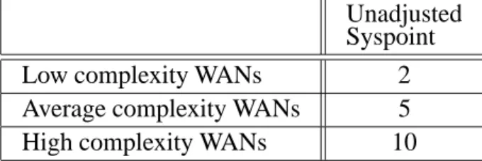
Table 9 represents the complexity matrix for the wide area network factors. Using the physi-cal categorization as the row and the functional categorization as the column, the cells of the matrix are filled with Low, Average, or High values. Table 10 represents the weights (
sys-point)assigned to each complexity of the wide
area network factors.
Based on the definition above of the low, ave-rage, and high complexity wide area networks, it is important that the total count of low, ave-rage, and high complexity wide area networks is determined. Using the unadjusted syspoint from the above table, a total wide area network unadjusted syspoint(λWAN) is then calculated
Unadjusted Syspoint
Low complexity WANs 2
Average complexity WANs 5
High complexity WANs 10
Table 10. WAN unadjusted Syspoint.
by multiplying the count of low, average, and high complexity printers with the corresponding unadjusted syspoint multiplier.
4.7. Server Application Factors
For the purpose of this study, the experts defined server applications as “the applications that are installed at the server to support tasks like Web, database, email and security”. The physical ca-tegories of the server component were identified as file and print, web, database, email, and secu-rity. The functional categories were identified as new installation, upgrade, and migration.
The file and print server was defined by an expert as follows: “A file server is a high-speed computer in a network that stores the programs and data files shared by users. It acts like a remote disk drive. A print server is a computer in a network that controls one or more printers. It is either part of the network operating system or an add-on utility that stores the print-image output from users’ machines and feeds it to the printer, one job at a time. The computer and its printers are known as a print server or a file server with print services”(Techweb, 2003).
The web server is a computer that provides World Wide Web services on the internet. A da-tabase server is a computer in a LAN dedicated to database storage and retrieval. The database server is a key component in a client/server
en-vironment. It holds the database management
Direct Routing Limited Access Fire-wall
Cable Modems Low Low Average High
ISDN/Frame relay Average Average High High
DS3/OC Average High High High
Wireless WAN Average High High High
system (DBMS) and the databases. Upon
re-quests from the client machines, it searches the database for selected records and passes them back over the network. For example – installa-tion and configurainstalla-tion of Oracle database on a LINUX Operating System.
An email server is a computer in a network that provides post office facilities. It stores incom-ing mail for distribution to users and forwards outgoing mail through the appropriate channel. The term may refer to just the software that performs this service, which can reside on a machine with other services. Example includes installation of Microsoft Exchange Server.
A security application that performs protection of the data against unauthorized access is gene-rally termed as security program. The instal-lation and configuration of such security appli-cations like the Firewall, and Access Control applications fall into this category.
The functional categories include new installa-tion, upgrade, and migration. New installation covers those projects where the installation and configuration of the application is performed from the scratch. Server application upgrade in-volves upgrade of different versions of the same application System. For example, an upgrade of Microsoft SQL Server 6 to SQL Server 7 is an upgrade installation. However, installations of patches or service packs are not covered by this sizing. They are considered normal main-tenance features and not installation projects.
The migration function involves migration from one application system to another application system. For example, a migration from a Mi-crosoft Exchange Server to a Lotus Notes Group-ware is covered by this classification.
Table 11 represents the complexity matrix for the server application factors. Using the physi-cal categorization as the row and the functional
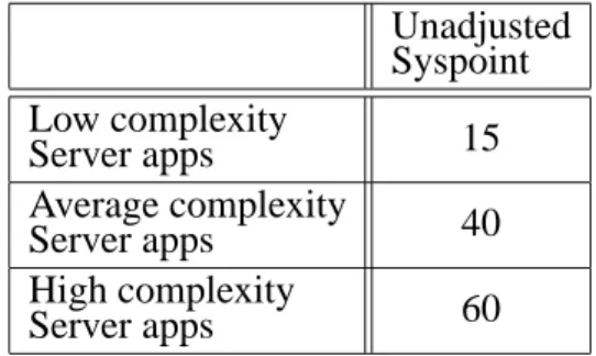
categorization as the column, the cells of the matrix are filled with Low, Average, or High values. Table 12 represents the weights (
sys-point)assigned to each complexity of the server
application factors.
Unadjusted Syspoint
Low complexity
Server apps 15
Average complexity
Server apps 40
High complexity
Server apps 60
Table 12. Server Application unadjusted Syspoint.
Based on the above definition of the low, ave-rage, and high complexity server applications, it is important that the total count of low, ave-rage, and high complexity server applications is determined. Using the unadjusted syspoint from the table above, a total server application unadjusted syspoint(λSa)is then calculated by
multiplying the count of low, average, and high complexity printers with the corresponding un-adjusted syspoint multiplier.
4.8. Client Application Factors
For the purpose of this study, the experts defined client application factor as “the applications that are installed on the workstation to support client tasks like word processing, remote sup-port, print and device software, and security”. The physical categories of the client application component were identified as a word process-ing/spreadsheet, remote support tools, database
client, printer software, fax/scan/imaging
soft-ware, video conferencing, security, email client,
New Installation Upgrade Migration
File and Print Low Low Average
Web Low Low Average
Database Average Average High
Email Average High High
Security High High High
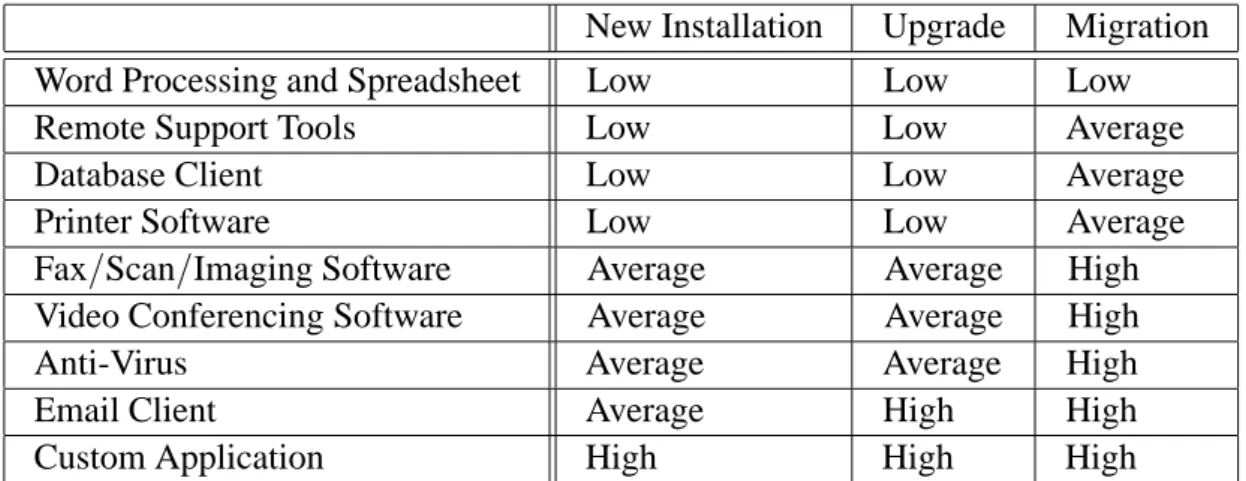
New Installation Upgrade Migration
Word Processing and Spreadsheet Low Low Low
Remote Support Tools Low Low Average
Database Client Low Low Average
Printer Software Low Low Average
Fax/Scan/Imaging Software Average Average High
Video Conferencing Software Average Average High
Anti-Virus Average Average High
Email Client Average High High
Custom Application High High High
Table 13. Client Application Complexity Matrix.
and custom application”. The functional cate-gories were identified as new installation, up-grade, and migration.
One of the experts defined the Word processing and spreadsheet category as follows: “Word Processing involves the creation of text docu-ments. Example: Microsoft Word, and Word Perfect. Spreadsheet is the software that simu-lates a paper spreadsheet(worksheet), in which
columns of numbers are summed for budgets and plans. It appears on screen as a matrix of rows and columns, the intersections of which are identified as cells. Example: Microsoft Excel, and Lotus 1–2–3”(Techweb, 2003).
Remote support tool is a software installed in both machines, that allows a user at a local com-puter to have control of a remote comcom-puter via modem. Both users run on the remote computer and see the same screen. Database client is a software that is provided by the database vendor and is required to be installed at the workstation for database connectivity purposes. Printer soft-ware is a softsoft-ware that is provided by the printer vendor and is required to be installed at the workstation for printer connectivity purposes. Fax or scan or imaging software is a software that is provided by the respective vendor and is required to be installed at the workstation for the connectivity purposes. Video conferencing is a software that is provided by the respec-tive vendor and is required to be installed at the workstation for video conferencing purposes. Anti virus is a software that is provided by the security vendor and is required to be installed at the workstation for detecting and blocking com-puter viruses. Example: Installation of Norton antivirus utility, and MacAfee antivirus utility.
Email client is a software that is provided by the respective vendor and is required to be in-stalled at the workstation, so that the users can access the email servers from local or remote networks. Example: Installation and configu-ration of Microsoft Outlook client. Custom ap-plications refer to the application that is specif-ically designed and programmed for an indivi-dual customer.
The functional categories include new instal-lation, upgrade, and migration. The descrip-tions of these functional categories are similar to those of the server application factors.
Table 13 represents the complexity matrix for the client application factors. Using the physi-cal categorization as the row and the functional categorization as the column, the cells of the matrix are filled with Low, Average, or High values. Table 14 represents the weights (
sys-point)assigned to each complexity of the client
application factors.
Unadjusted Syspoint
Low complexity
Client apps 4
Average complexity
Client apps 7
High complexity
Client apps 11
Table 14. Client Application unadjusted Syspoint.
and high complexity client applications is deter-mined. Using the unadjusted syspoint from the above table, a total client application unadjusted syspoint(λCa)is then calculated.
4.9. Handheld Application Factor
For the purpose of this study, the experts de-fined handheld application as follows: “The custom applications that are installed in the handheld devices on top of the OEM installed operating system are referred to as handheld applications”. The physical categories of the handheld component were identified as a local network, database, and web based. The func-tional categories were identified as basic instal-lation, phone, and wireless. The local network handheld application is stand-alone and requires simple local USB or Serial “Sync” based com-munication configuration. A database-related handheld application refers to those applica-tions that involve storage and retrieval of in-formation, both from a local database and from a database stored at a remote server. A web-based handheld application represents those ap-plications that are web-based and uses wireless access protocols and architecture to display the information in the handheld. The customiza-tion of such applicacustomiza-tions may require addicustomiza-tional steps and intensive testing procedures.
The functional categories include basic instal-lation, phone, and wireless. Basic installation covers those projects that involve simple in-formation input, and query application. The phone installation represents those applications that use the phone capabilities of the handheld. The wireless installation represents those appli-cations that use the wireless capabilities of the handheld.
Basic Phone Wireless
Local
Network Low Low Average
Database Low Average High
Web-based Average High High
Table 15. Handheld Application Complexity Matrix.
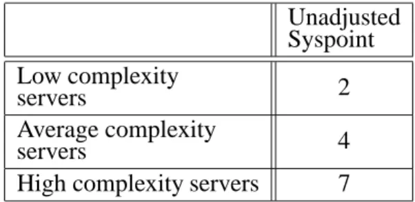
Table 15 represents the complexity matrix for the handheld application factors. Using the physical categorization as the row and the func-tional categorization as the column, the cells
of the matrix are filled with Low, Average, or High values. Table 16 represents the weights
(syspoint) assigned to each complexity of the
handheld application factors.
Unadjusted Syspoint Low complexity
servers 2
Average complexity
servers 4
High complexity servers 7
Table 16. Handheld Application unadjusted Syspoint.
Based on the above definition of the low, ave-rage, and high complexity handheld application, it is important that the total count of low, ave-rage, and high complexity handheld application is determined. Using the unadjusted syspoint from the above table, a total handheld appli-cation unadjusted syspoint(λHa)is then
calcu-lated.
4.10. Unadjusted Project Syspoint
A total unadjusted syspoint is calculated for each of the factors using the syspoint worksheet as the guideline. The sum of all those total un-adjusted syspoints will result in the unun-adjusted project syspoint(ΛPROJ). The formula for
com-puting the unadjusted project syspoint is given below.
ΛPROJ=λS+λW+λP+λLAN+λWAN
+λSa+λCa+λHa:
WhereΛPROJis the project unadjusted syspoint,
4.11. Adjusted Project Syspoint
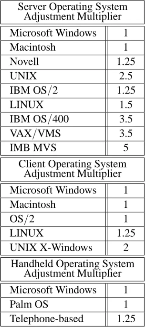
The operating systems play a large role in de-termining the size of the project. The unadju-sted project syspoint provides the size to of the project without taking this factor into considera-tion. The purpose of the unadjusted project sys-point is to analyze and compare projects without any additional dimension added by the operat-ing system.
Operating systems bring an additional dimen-sion to the sizing equation. The operating sys-tem impacts the server, workstation, and hand-held factors. For example, if an IT infrastruc-ture project involves installation of 5 servers, and 2 out of 5 are low complex servers, 2 avera-ge complex servers and 1 high complex server. Assume that, of the 2 low complex servers, 1 is a Microsoft Windows operating system and the other is a UNIX operating system. Hence it will be difficult to use one categorization and
Server Operating System Adjustment Multiplier
Microsoft Windows 1
Macintosh 1
Novell 1.25
UNIX 2.5
IBM OS/2 1.25
LINUX 1.5
IBM OS/400 3.5
VAX/VMS 3.5
IMB MVS 5
Client Operating System Adjustment Multiplier
Microsoft Windows 1
Macintosh 1
OS/2 1
LINUX 1.25
UNIX X-Windows 2
Handheld Operating System Adjustment Multiplier
Microsoft Windows 1
Palm OS 1
Telephone-based 1.25
Table 17. Operating System Adjustment Multiplier.
apply it to the other. The sizing of IT infras-tructure projects is really not a straight forward two dimensional matrix.
To simplify the calculation, the experts sug-gested using the sizing worksheet for each ope-rating system separately. In the above example, the unadjusted server syspoint would be calcu-lated twice – once for 1 low complexity server and adjusted to the Microsoft Windows opera-ting system, and again for 1 low complexity server adjusted to the UNIX operating system.
Operating system adjustment multipliers are provided in the table below. These weights are multipliers and are identified based on Mi-crosoft Windows operating system as the base-line. In other words, the unadjusted project syspoint will not change if the project only uses Microsoft Windows as the operating system in the project. The multipliers are determined by the experts based on their past experience.
The adjusted syspoint for the server(λ
S(adj) )is
calculated by multiplying the unadjusted server syspoint (λS) with the adjustment multiplier.
The adjusted syspoint for the workstation
(λ
W(adj)
) is calculated by multiplying the
un-adjusted workstation syspoint (λW) with the
adjustment multiplier. The adjusted syspoint for the handheld (λ
Ha(adj)
) is calculated by
multi-plying the unadjusted handheld application sys-point(λHa)with the adjustment multiplier. The
adjusted syspoint for the project is calculated by adding the three adjusted syspoints to the other five unadjusted syspoints.
ΛPROJ(ADJ)
=λ
S(adj) +λ
W(adj)
+λP+λLAN +λWAN+λSa+λCa+λ
Ha(adj)
Where ΛPROJ(ADJ) is the project adjusted
sys-point, λS(adj) is the total adjusted server
sys-point,λW(adj) is the total adjusted workstation
syspoint,λPis the total unadjusted printer sys-point, λLAN is the total unadjusted LAN sys-point,λWAN is the total unadjusted WAN sys-point,λSais the total unadjusted server applica-tion syspoint,λCa is the total unadjusted client application syspoint, and λHa(adj) is the total
4.12. Limitations of Study
The non existence of a sizing model for IT in-frastructure project forced the usage of a quali-tative brain storming method like a focus group to develop a model. The method of selection of the focus group experts is not based on statisti-cal sampling technique. However, this method is valid when the objective of the study is not to perform any statistical tests. This method is described as theoretical sampling until satu-ration (Glaser and Strauss, 1967). The study
stopped with developing the model. The testing of the model will be conducted by another study which will be quantitative in nature.
This study focused on the IT infrastructure project-related sizing factors. The generic pro-ject factors were not included into the scope of the study. The generic project factors such as the expertise of resources, risk factors, critical na-ture of the project, and government project can influence the sizing of any project. Since this is the first study involved in developing an IT in-frastructure sizing model, these generic factors were purposefully placed outside the scope of the study.
5. Conclusion
The focus group of experts discussed the ad-vantages of having a sizing model and its ap-plication in their professional environment. In answering to the discussion question about the current sizing process, one of the experts com-mented, “:::It allows me to relate to what is
missing in our area. Even with the results we have identified so far, I am sure, I will be able to manage my projects better”.
This comment allowed expanding the thought process of how the sizing model will allow the IT infrastructure project managers to manage their projects better. Hence a discussion ques-tion, “That is an important point that I would like to capture in detail. Why do you feel that you will be able to manage your projects bet-ter?” was raised. This discussion question had a lot of comments and they are discussed in de-tail below as they pertain to the application of syspoint in the project environment.
The first reply to this question was, “In the area of infrastructure projects, as you very well
know, we don’t have tools similar to that of soft-ware development projects. That does not mean that we don’t carry out large projects. Without proper tools to do sizing, estimation, and com-parison, we have to rely on our expert judgment. It helps to have an objective measure, docu-ment the procedure and allow the team mem-bers do the sizing, and estimation of projects us-ing bottom-up technique. Most of my projects have been estimated just by me or with my ma-nager. Top-down approach – even though it is faster, could mean lack of team members’ buy-in. With a quantitative measure, as a mana-ger, I will be able to make the team participate in this process, groom other members in esti-mation, improve team motivation etc. This will have a positive effect on the team members in various areas. This will make a difference for infrastructure project managers”.
Another expert added, “Absolutely, this is an important research in the infrastructure area. Currently, grooming junior project managers in the infrastructure area is a difficult task. Since the key project management activities are per-formed using subjective approach, it becomes difficult to train junior project managers. Most training happens on-the-job. We have to learn through mistakes. If techniques and methods similar to software development area exist, we will be able to conduct a training class and teach them how to perform these activities instead of relying on them picking my brain”.
In replying to this comment, another expert said, “Also, don’t forget about the power of using an objective approach when trying to justify the es-timates. Currently, it is subjective and requires a lot of justification on how we come up with the numbers we come up with. It is sometimes difficult to make the senior management un-derstand expert judgment has some ’judgment’ factor involved”.
Based on this discussion, the following advan-tages of the syspoint measure were identified
Objective estimation technique
Consistency in estimation within the organi-zation
Ability to compare IT infrastructure projects within or between organizations
Ability to implement bottom-up estimating technique
Ability to justify the estimates to the senior management
Ability to calibrate based on the organiza-tional experience
Improve team buy-in and increase motiva-tion among team members
The study offers a lot of scope for future research. Testing of this model is the first step. The next step would be to include the generic project sizing factors into the equation. Further-more, extending this model to develop effort es-timation and cost eses-timation can be performed using quantitative research techniques. Sche-dule estimation can also be performed based on a high level work break down structure for IT infrastructure projects.
Acknowledgment
The authors would like to thank the editors and reviewers of CIT for their positive feedback about the SYSPOINT research and for reco-gnizing SYSPOINT as a valuable addition to the body of knowledge.
References
1] A. ABRAN, M. MAYA& D. DESHARNAIS, Adapting function points to real-time software. American
Programmer, November(1997), pp. 32–42. 2] S. R. CHIDAMBER& C. F. KEMERER, A Metrics suite
for object-oriented design. IEEE Transactions on
software engineering, June(1994), pp. 476–493. 3] J. B. DREGER, Function point analysis. Englewood
Cliffs, NJ, Prentice Hall, 1989.
4] D. FERENS, Software size estimation: Quo Vadis?
National Estimator, Winter(1999), pp. 43–54. 5] Function point counting practices manual, 2000,
IFPUG
6] B. G. GLASER& A. L. STRAUSS, The Discovery of
Grounded Theory, Chicago, Aldine Publishing Co.,
1967.
7] J. JOHNSON, K. BOUCHER, K. CONNORS, K., & J. ROBINSON, Collaborating on Project Success,
Soft-ware Magazine, Mar(2001).
8] T. JONES, Programming productivity, New York, McGraw Hill, 1986.
9] S. LIU, practical framework for discussing IT in-frastructure, IT Pro, Aug(2002), pp. 14–21.
10] K. PETERS, Software Project Estimation, Vancouver, CA, Software Productivity Center, 1999.
11] Techweb 2003. The Business technology network: TechEncyclopedia(Online), Available,
http://www.techweb.com/encyclopedia/
Received: August, 2003 Accepted: March, 2004
Contact address:
Srinivasa Raghavan President Krea Corporation 3471 Wilkes Drive Naperville, IL-60564 USA e-mail:[email protected]
Veeraswamy Achanta President Rangasoft Corporation 178 Michigan Court Bloomingdale, IL-60108 USA e-mail:[email protected]
SRINIVASARAGHAVANworks as a President of Krea Corporation, an IT and management consulting firm located in Illinois, USA. He also func-tions as a mentor at the School of Business, NorthCentral University and as a faculty at the School of Technology, Capella University. He has a BS in Mathematics from the University of Madras, a MS in Computer Applications from the University of Madras, an MBA in International Business from Keller Graduate School of Management, a MS in Project Management from Keller Graduate School of Management and a PhD in Organization and Management with specialization in IT, from Capella University. Raghavan’s research interests include IT project estimation models, decision support systems, operation research, project manage-ment, qualitative research techniques – in particular online methods, and IT life cycle models.