Does It Really Pay to Be Green?

© Copyright 2001 by the

Massachusetts Institute of Technology and Yale University

Volume 5, Number 1

Does It

Really

Pay

to Be Green?

An Empirical Study of Firm Environmental

and Financial Performance

Andrew A. King and Michael J. Lenox

Keywords beyond compliance corporate strategy econometric analysis environmental performance Porter hypothesis win-win

Address correspondence to: Michael Lenox

Stern School of Business New York University 40 West 4th St. Suite 717 New York, NY 10012 [email protected] www.stern.nyu.edu/˜mlenox/

Summary

Previous empirical work suggests that Žrms with high environ-mental performance tend to be proŽtable, but questions per-sist about the nature of the relationship. Does stronger envi-ronmental performance really lead to better Žnancial performance, or is the observed relationship the outcome of some other underlying Žrm attribute? Does it pay to have clean-running facilities or to have facilities in relatively clean industries? To explore these questions, we analyze 652 U.S. manufacturing Žrms over the time period 1987±1996. Al-though we Žnd evidence of an association between lower pol-lution and higher Žnancial valuation, we Žnd that a Žrm’s Žxed characteristics and strategic position might cause this associa-tion. Our Žndings suggest that " When does it pay to be green?" may be a more important question than " Does it pay to be green?"

Scholars had long assumed that investments to protect the natural environment provided few Ž-nancial beneŽts to Žrms. In the last 20 years, however, a growing number of researchers have challenged this assumption. In the Želd of in-dustry ecology, scholars argue that there are sit-uations where beyond-compliance behavior by Žrms is a win-win for both the environment and the Žrm (Nelson 1994; Panayotou and Zinnes 1994; Esty and Porter 1998; Reinhardt 1999). Scholars now suggest that Žrms may be both green and competitive (Porter and van der Linde 1995; Reinhardt 1999). Qualitative research has identiŽed numerous examples of proŽtable pol-lution prevention opportunities (Denton 1994; Deutsch 1998; Graedel and Allenby 1995; Porter and van der Linde 1995; King 1995). Many scholars now argue that discretionary improve-ments in environmental performance often pro-vide Žnancial beneŽt (e.g., Hart 1997).

In response, a growing empirical literature shows that researchers have applied econometric techniques to test the “pays to be green” hypoth-esis. Several studies have provided evidence that higher environmental performance is associated with better Žnancial performance, but these early studies often lacked the longitudinal data needed to fully test the relationship. Several years of data are needed if one wants to rule out rival expla-nations for the apparent association or show that environmental improvement causes Žnancial gain. Furthermore, the empirical literature does not clarify whether the apparent association is generated by a Žrm’s choice to operate in cleaner industries or to operate cleaner facilities. Existing research cannot answer whether it pays to be green or whether it pays to operate in green in-dustries.

In this article, we review and comment on the empirical “pays to be green” literature. We dis-cuss how a Žrm’s stable attributes (i.e., the char-acteristics of the Žrm that persist over time) and strategic position may jointly cause both lower pollution levels and better Žnancial performance and thereby create the appearance of a direct re-lationship between the two. For example, inno-vative Žrms may have both lower emissions lev-els and greater proŽts. Alternatively, managers may choose to improve their Žrm’s

environmen-tal performance when they have an especially proŽtable year.

To help distinguish the effect of pollution re-duction from other underlying factors, we adopt empirical methods that account for unmeasured Žrm attributes. Furthermore, to differentiate be-tween pollution reduction and divestiture of operations in dirtier industries, we separate en-vironmental performance into two constructs: 1) relative performance within a given industry and 2) the average performance of the industries in which one chooses to operate. We analyze 652 U.S. manufacturing Žrms over the time period 1987 –1996. We Žnd evidence of a real associa-tion between lower polluassocia-tion and higher Žnan-cial performance. We also show that a Žrm’s en-vironmental performance relative to its industry is associated with higher Žnancial performance. We cannot show conclusively, however, that a Žrm’s choice to operate in cleaner industries is associated with better Žnancial performance, nor can we prove the causal direction of the observed relationships. Thus, our research provides sup-port for a connection between some means of pollution reduction and Žnancial performance, but it also suggests that the reason for this con-nection remains to be established.

Evidence to Date

Proponents of a causal link between environ-mental and Žnancial performance have argued that pollution reduction provides future cost sav-ings by increasing efŽciency, reducing compli-ance costs, and minimizing future liabilities (Por-ter and van der Linde 1995; Reinhardt 1999). Porter and van der Linde (1995) theorized that opportunities for proŽtable pollution reduction exist because managers often lack the experience and skill to understand the full cost of pollution (Jaffe et al. 1995). Hart (1997) proposes that ex-cess returns (i.e., proŽts above the industry av-erage) result from differences in the underlying environmental capabilities of Žrms. Managers may possess unique resources or capabilities that allow them to employ proŽtable environmental strategies that are difŽcult to imitate.

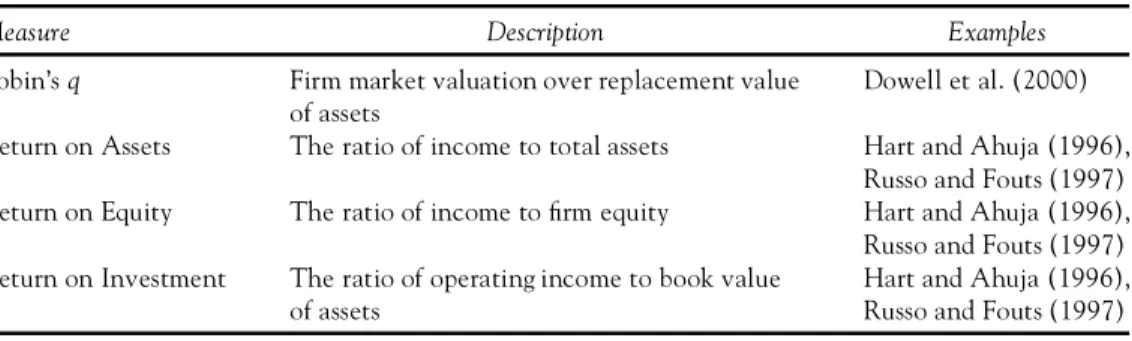
Using a variety of measures (tables 1 and 2), much of the empirical “pays to be green”

litera-Table 1 Measures of corporate Žnancial performance used in ª pays to be greenº scholarship

Measure Description Examples

Tobin’sq Firm market valuation over replacement value

of assets Dowell et al. (2000)

Return on Assets The ratio of income to total assets Hart and Ahuja (1996), Russo and Fouts (1997) Return on Equity The ratio of income to Žrm equity Hart and Ahuja (1996),

Russo and Fouts (1997) Return on Investment The ratio of operating income to book value

of assets Hart and Ahuja (1996),Russo and Fouts (1997)

Table 2 Measures of corporate environmental performance used in ªpays to be greenº scholarship

Measure Examples

Capital expenditures on pollution control technology Spicer (1978) Nehrt (1996) Emissions of toxic chemicals (typical source: TRI) Hamilton (1995)

Hart and Ahuja (1996)

Spills and other plant accidents Karpoff et al. (1998)

Lawsuits concerning improper disposal of hazardous waste Muoghalu et al. (1990) Rewards or other recogition for superior environmental performance Klassen and McLaughlin (1996) Participation in environmental management standards White (1996)

Dowell et al. (2000) Rankings of superior environmental performers (e.g., CEP) White (1996)

Russo and Fouts (1997) ture has supported the proposed positive

rela-tionship between pollution reduction and Žnan-cial gain by relying on correlative studies of environmental and Žnancial performance. A se-ries of studies conducted by the Council on Eco-nomic Priorities (CEP) in the 1970s found that expenditures on pollution control were signiŽ-cantly correlated with Žnancial performance among a sample of pulp and paper Žrms (Spicer 1978).1_{More recently, Russo and Fouts (1997)}

found a signiŽcant positive correlation between various Žnancial returns and an index of envi-ronmental performance developed by the CEP. Dowell and colleagues (2000) found that Žrms that adopt a single, stringent environmental standard worldwide have higher market valu-ation (Tobin’s q) than Žrms that do not adopt such standards.

In the Žnance literature, a number of studies have examined the market returns of portfolios of environmentally friendly Žrms. Cohen and colleagues (1995) used several measures of en-vironmental performance derived from U.S.

En-vironmental Protection Agency (U.S. EPA) da-tabases to construct two industry-balanced portfolios of Žrms. They found no penalty for in-vesting in the green portfolio and a positive re-turn to green investing. Similarly, White (1996) found a signiŽcantly higher risk-adjusted return for a portfolio of green Žrms using the CEP rat-ings of environmental performance.2

To the extent that one cares merely about cor-relation and little about causation, these correl-ative studies are informcorrel-ative. Market analysts, for example, increasingly gather environmental per-formance data as an indicator of future capital market returns (Kiernan 1998). For their pur-poses, it matters little whether environmental performance leads to Žnancial performance or simply provides an indicator of Žrms that have high Žnancial performance.

From the perspective of corporate managers and policy analysts, however, the distinction is critical. The prescription that often follows from the “pays to be green” literature is that managers should make investments to lower their Žrm’s

en-vironmental impact (Hart and Ahuja 1996). To fully demonstrate that it pays to be green, re-search must demonstrate that environmental im-provements produce Žnancial gain.

Event studies are one means of demonstrating that greening indeed causes Žnancial gain. Such studies look at the relative changes in stock price following some environmental event. By isolat-ing a sisolat-ingle environmental event within a narrow time frame, event studies control for important differences among Žrms that cannot be observed. The limitation with event studies is that they often study the effect of events that are only par-tially environmental in nature. Klassen and McLaughlin (1996), White (1996), Karpoff and colleagues (1998), and Jones and Rubin (1999) studied the effect of published reports of events and awards on Žrm valuation and found a rela-tionship between the valence of the event (posi-tive or nega(posi-tive) and the resulting change in market valuation. Blacconiere and Patten (1994) estimated that Union Carbide lost $1 billion in market capitalization, or 28%, following the Bhopal chemical accident in 1984. Muoghalu and colleagues (1990) found that Žrms named in lawsuits concerning improper disposal of hazard-ous waste suffered signiŽcant losses in capital market value. Each of these events has environ-mental elements, but each is affected by other Žrm attributes. King and Baerwald (1998) argued that size, market power, and unique Žrm char-acteristics inuence how events are reported and interpreted. A Žrm with good public relations may be able to put a positive spin on negative news. A Žrm that possesses good legal resources may better forestall lawsuits.

In some event studies, researchers have sought to avoid these problems by using the an-nual release of toxic emission data through the U.S. EPA’s Toxic Release Inventory (TRI) pro-gram as the event. Hamilton (1995), Konar and Cohen (1997), and Khanna and colleagues (1998) all found that polluting Žrms lost market value in a one-day window following the release of TRI information. These important studies still may suffer from construct validity, however. Given the complexity of analyzing TRI data, it seems possible that same-day stock price move-ments probably reect contemporaneously re-ported pollution rankings. These rankings are

strongly affected by Žrm size and industry choice, and thus the stock market effect may be the re-sult of temporary bad press rather than a real change in perception of a Žrm’s long-term value. In fact, stock values often return to pre-event levels within a Žve-day window following the TRI data release. Proponents of event studies, however, claim that the return of the price to pre-event levels is most likely to be a response to new, unrelated information.

Another way to account for unobserved Žrm differences is to use standard regression tech-niques to evaluate the effect of changes in pol-lution on changes in Žnancial performance. This in essence is the approach used in a widely cited study by Hart and Ahuja (1996). They showed that changes in pollution (emission per sales dol-lar) predate changes in Žnancial performance. Although an important advance in the literature, their measure of environmental performance conates reduction of pollution at current opera-tions and divestiture of dirty operaopera-tions, making it difŽcult to interpret the meaning of their study. Is it that it pays to be green or does it pay to operate in clean industries?

This issue underscores a larger debate within the strategy literature on the source of returns in excess of investments of similar risk (Rumelt 1991; McGahan and Porter 1997). The indus-trial organization literature in economics suggests that excess returns result from differences in the underlying structure of industries. According to this logic, greener industries may have higher re-turns than dirtier industries because of lower compliance and regulatory costs. In contrast, the resource-based view of strategic management suggests that individual Žrm capabilities may lead to excess returns when they are difŽcult to imi-tate, not substitutable, rare, and valuable (Bar-ney 1986; Wernerfelt 1984). According to this view, superior ability to manage environmental problems relative to others in your industry may lead to higher returns. In much of the empirical “pays to be green” literature, researchers have used strategy resource-based logic to justify a re-lationship between environmental and Žnancial performance. Unfortunately, they fail to disen-tangle the effects of industry choice from the ef-fects of variation in environmental strategies among Žrms in the same industry.

An Empirical Approach

In the following sections, we analyze whether it really “pays to be green” using a methodology that allows us to explore whether unmeasured Žrm and industry characteristics may explain the observed link between environmental and Žnan-cial performance. We also use a measure of en-vironmental performance that untangles the ef-fect of a Žrm’s relative performance within its industries and the average performance of the in-dustries in which it chooses to be.

We created a sample of publicly traded U.S. manufacturing Žrms during the period 1987– 1996 by combining the U.S. EPA’s Toxic Release Inventory (TRI) with facility data from Dun & Bradstreet and corporate data from Standard & Poor’s Compustat database. The U.S. EPA started the TRI in 1987 to track emissions of more than 200 toxic chemicals from U.S. manu-facturing Žrms. Facilities must complete annual TRI reports if they manufacture or process 25,000 pounds (or about 11,340 kg), use more than 10,000 pounds of any listed chemical during a calendar year, and employ ten or more full-time people. To be in our sample, a Žrm must have at least one facility that meets these requirements and be among the public corporations listed in the Compustat database. Matching the two sets, we created an unbalanced sample of 652 Žrms constituting 4,483 Žrm-year observations for the years 1987 through 1996.3

Measures

Financial Performance

The dependent variable for our analysis is Ž-nancial performance as reected by Tobin’s q.

Tobin’sqmeasures the market valuation of a Žrm relative to the replacement costs of tangible as-sets (Lindenberg and Ross 1981). Essentially, it reects what cash ows the market thinks a Žrm will provide per dollar invested in assets. It should be higher if future cash ows are expected to be greater or if they are expected to be less risky. In accordance with more recent “pays to be green” studies, we use a simpliŽed measure of Tobin’s q (Dowell et al. 2000). We calculated Tobin’s q by dividing the sum of Žrm equity value, book value of long-term debt, and net

cur-rent liabilities by the book value of total assets.4

All Žnancial data were obtained from the Com-pustat database.

Environmental Performance

Previous research has measured the environ-mental performance of a Žrm as the degree to which that Žrm emits toxic pollution given its size (Hart and Ahuja 1996). We create a similar measure (Total Emissions) by calculating the log of total facility emissions of toxic chemicals. Un-fortunately, the meaning of this variable is am-biguous because it confounds pollution that re-sults from industry positioning with pollution that results from poor environmental manage-ment. Consequently, we form two additional variables to separate the effect of environmental management from the effect of industry position-ing.Relative Emissionsmeasures the Žrm’s ability to manage and reduce its pollution by comparing the degree to which a Žrm’s facilities are more or less polluting than other facilities in the same industry (measured by the four-digit Standard In-dustrial ClassiŽcation (SIC) code and adjusted for differences in size). Industry Emissions mea-sures the degree to which a Žrm tends to operate in industries where production entails pollution. If a Žrm operates in industries where the average facility has higher emissions, this variable will have a larger value. Please refer to the appendix for a detailed description of the construction of these variables.

Controls

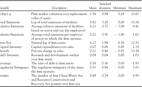
We include a number of measures commonly used in the analysis of Žnancial performance as controls (tables 3 and 4). These measures include 1) the company’s size (Firm Size) calculated as the log of the company’s assets, 2) the capital intensity of a Žrm (Capital Intensity) calculated by dividing capital expenditures by sales, 3) the annual growth of the Žrm (Growth) calculated as the percentage change in sales, 4) the degree to which the Žrm is leveraged (Leverage) divided as the ratio of its debt to assets, and 5) the research and development intensity (R&D Intensity) cal-culated by dividing research and development expenses by total assets.

In addition, we control for the stringency of the regulatory environment in which the Žrm

Table 3 Descriptive statistics

Variable Description Mean

Standard

deviation Minimum Maximum

Tobin’sq Firm market valuation over replacement value of assets

1.58 0.94 0.28 12.67

Total Emissions Log of total emissions of facilities 5.82 3.28 0.00 13.76 Relative Emissions Average relative emissions of facilities

based on sector and size (in employees) 0.21 0.77 – 7.08 9.41 Industry Emissions Average total emissions per employee

of sectors in which the Žrm operates 0.22 0.50 – 1.80 1.62

Firm Size Natural log of Žrm assets 6.27 1.94 0.76 12.52

Capital Intensity Capital expenditures over sales 0.07 0.06 0.00 1.19

Growth Percent change in sales 0.12 0.44 – 0.91 13.36

R&D Intensity Research and development outlays over Žrm assets

0.04 0.04 0.00 1.03

Leverage The ratio of debt to Žrm assets 0.18 0.16 0.00 1.93

Regulatory Stringency The regulatory stringency of the states the Žrm operates

0.51 0.84 0.00 7.01

Permits The number of Žrm Clean Water Act and Resource Conservation and Recovery Act permits over Žrm size

0.49 0.74 0.00 5.95

Note: n= 4,483.

operates (Regulatory Stringency). Environmental regulation varies across regions and imposes greater (or lesser) penalties for pollution from fa-cilities operating in those regions. We measure a state’s regulatory stringency by calculating the inverse of the log of toxic emissions divided by total employees in four main polluting industries: chemicals, petroleum, pulp and paper, and ma-terials processing (Meyer 1995). The logic for this measure is that higher regulation leads to lower emissions per employee (for these indus-tries) and thus increases the inverse of this ratio (Regulatory Stringency). For each Žrm, we create a measure of the average regulation it faces by calculating the weighted-average of the regula-tory stringency for all the states in which the Žrm operates.

To create an alternative measure of the degree to which the different facilities in our sample are regulated, we count the number of performance criteria with which each facility must comply (i.e., the number of permits issued to a facility). Under the U.S. Clean Water Act (CWA 1977), regulators may impose limits on water ow, sus-pended solids, and chemical concentration. Al-though guidelines exist for administering the law,

substantial discretionary power remains. We cre-ated an alternative measure of regulatory strin-gency,Permits,by summing the number of federal permits and then dividing by Žrm size.

Results

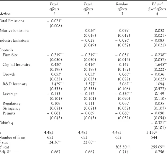
Previous studies have found that pollution precedes poor Žnancial performance by one or more years (Hart and Ahuja 1996). To test these Žndings, we use least-squares regression analysis to Žnd a linear relationship between our inde-pendent variables and the Žrm’s future Tobin’sq

(table 5).5_{Because Žrms may differ in ways that}

we do not capture with our independent vari-ables, we include dummy variables that allow each Žrm to have a different constant value. This is often called a “Žxed effects” analysis because it reduces the possibility that a Žrm’s Žxed attri-butes confound the analysis. In essence, this Žxed-effect regression requires that changes in independent variables (rather than their baseline level) be associated with changes in dependent variables.

Consistent with much of the “pays to be green” literature, we Žnd that Total Emissionsis

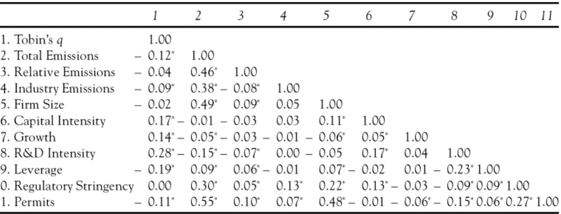
Table 4 Correlations

1 2 3 4 5 6 7 8 9 10 11

1. Tobin’sq 1.00

2. Total Emissions – 0.12* 1.00 3. Relative Emissions – 0.04 0.46* _1.00 4. Industry Emissions – 0.09* _0.38*_{– 0.08}* _1.00 5. Firm Size – 0.02 0.49* _0.09* _{0.05 1.00} 6. Capital Intensity 0.17*_{– 0.01 – 0.03 0.03 0.11}* _1.00 7. Growth 0.14*_{– 0.05}*_{– 0.03 – 0.01 – 0.06}* _0.05* _1.00 8. R&D Intensity 0.28*_{– 0.15}*_{– 0.07}* _{0.00 – 0.05 0.17}* _{0.04 1.00} 9. Leverage – 0.19* _0.09* _0.06*_{– 0.01 0.07}*_{– 0.02 0.01 – 0.23}*_1.00 10. Regulatory Stringency 0.00 0.30* _0.05* _0.13* _0.22* _0.13*_{– 0.03 – 0.09}*_0.09*_1.00 11. Permits – 0.11* 0.55* 0.10* 0.07* 0.48*– 0.01 – 0.06*– 0.15*0.06*0.27*1.00 Note: n= 4,483.

*_{p< 0.001.}

associated with superior Žnancial performance even when controlling for Žrm Žxed effects (model 1). Thus, we provide evidence that en-vironmental performance is associated with Ž-nancial performance rather than the observed re-lationship being the outcome of some other underlying Žrm attribute.

As discussed earlier, evidence of such a rela-tionship still leaves many unanswered questions. Does it pay to have clean-running facilities, or to have facilities in relatively clean industries? To better account for these differences, we separate

Total Emissionsinto two parts that reect a Žrm’s tendency to operate in polluting industries ( In-dustry Emissions) and its tendency to operate dirt-ier facilities within these industries (Relative Emissions). In model 2, the signiŽcant and neg-ative coefŽcient for Relative Emissions indicates that Žrms with lower emissions in their industries tend to experience higher Žnancial performance in the subsequent year. The lack of signiŽcance for the coefŽcient for Industry Emissions means that we cannot conclude that Žrms that operate in cleaner industries have higher Žnancial per-formance.

One problem with Žxed effects analysis is that it can do its job too well. By eliminating the ef-fect of all Žrm attributes that are relatively con-stant, the Žxed effect may obscure evidence that a Žxed attribute is actually important. If Žrms do not frequently change industry, and thus industry position is relatively constant, we might miss the

Žnancial effect of industry choice. To check this, we use an alternative speciŽcation called “ran-dom effects.” Although this method continues to reduce the effect of Žxed Žrm attributes, it as-sumes that these are normally distributed. This method suggests that Žrms that operate in cleaner industries (Industry Emissions) have higher Žnancial performance.

What might explain the difference between model 3 and model 2? One possibility is that few Žrms in our sample actually move across indus-tries, and thus the Žxed effects analysis removes the effect of industry position. Another possibil-ity is that Žrms beneŽt from being in cleaner in-dustries but not from moving to cleaner indus-tries. Perhaps such movement entails costs that reduce a Žrm’s valuation or signals some difŽculty or problem. It is important to note that in our particular case, statistical tests suggest that the Žxed effects and not random effects analysis should carry more credence.6

Finally, we still have not considered the effect of causality. Which way does the relationship run? Do more-proŽtable Žrms invest more in en-vironmental performance, or does environmen-tal performance lead to proŽt? In model 4, we present one method for answering this question. To reduce the effect of a previous proŽtable year, we include the previous year’s Tobin’sq in the regression.7_{Unfortunately, this analysis does not}

provide reliable evidence that Žrms with lower emissions in their industries (Relative Emissions)

Table 5 Estimates of future Žnancial performance (Tobin’sqt+1) 1987±1996

Method

Fixed effects 1

Fixed effects 2

Random effects

3

IV and Žxed effects

4

Total Emissions – 0.021** (0.008)

Relative Emissions – 0.036*

(0.018) – 0.029

+

(0.017) – 0.032(0.021)

Industry Emissions – 0.027

(0.049) – 0.076

*

(0.037) – 0.083(0.021) Controls

Firm Size – 0.219***

(0.030) – 0.219

***

(0.030) – 0.034

*

(0.014) – 0.238

*** (0.057) Capital Intensity – 0.420*

(0.198)

– 0.416* (0.198)

– 0.147 (0.187)

– 1.645*** (0.222)

Growth 0.053*

(0.022) 0.053

*

(0.023) 0.068

**

(0.022) – 0.036(0.022) R&D Intensity 3.429***

(0.535) 3.377

***

(0.535) 5.062

***

(0.408) (0.577)1.094

Leverage – 0.153

(0.101) – 0.152(0.101) – 0.330 ***

(0.090) (0.110)0.149 Regulatory

Stringency

0.108 (0.071)

0.111 (0.071)

0.080* (0.032)

0.035 (0.107)

Permits – 0.061

(0.045) – 0.069(0.045) – 0.060

+

(0.032) – 0.090(0.054)

Tobin’sq – 0.321***

(0.101)

n 4,483 4,483 4,483 3,130a

Number of Žrms 652 652 652 544

Fstat 24.36*** _22.80***

2_{stat 505.30}*** _255.09***

Adj.R2 _{0.667 0.667 0.714 0.756}

Note:Firm and year dummies are included but not presented in all models. Standard errors are in parentheses.

a_{The sample is slightly smaller because of the inclusion of lagged instruments.}

+ _{p< 0.10,}*_{p< 0.05,}**_{p< 0.01,}***_{p< 0.001 (two-tailed test).}

tend to experience higher Žnancial performance. Thus, although we Žnd evidence of an associa-tion between reduced emissions and proŽt, we cannot say with conŽdence which way the rela-tionship runs. We again Žnd no evidence that the cleanliness of the industries in which the Žrm has facilities (Industry Emissions) is associated with higher market valuation when we control for Žrm Žxed effects.

The above analysis is illustrative of what we found throughout our analysis. Using different forms of models and different methods for mea-suring our variables, we often found an associa-tion between environmental and Žnancial

per-formance; however, we also found that variations in model speciŽcation, sample, and measurement method could reduce the signiŽcance of this ef-fect below accepted thresholds (although it never reversed in sign). Out of the population of models we estimated, we have presented the most careful speciŽcations and robust results.

Conclusions

In this paper, we further explore whether it “pays to be green.” We use longitudinal data and statistical methods that reduce the potential for unobserved differences among Žrms to create a

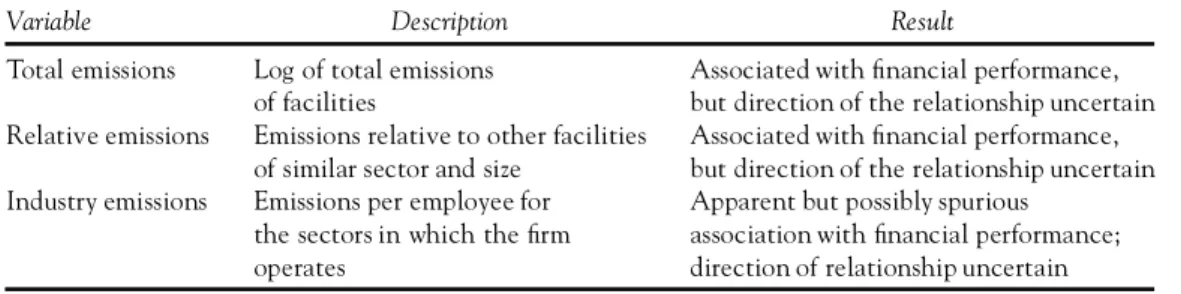
Table 6 Summary of Žndings

Variable Description Result

Total emissions Log of total emissions

of facilities Associated with Žnancial performance,but direction of the relationship uncertain Relative emissions Emissions relative to other facilities

of similar sector and size

Associated with Žnancial performance, but direction of the relationship uncertain Industry emissions Emissions per employee for

the sectors in which the Žrm operates

Apparent but possibly spurious association with Žnancial performance; direction of relationship uncertain

misleading association between environmental and Žnancial performance. We also test to see whether pollution reduction causes Žnancial gain. Table 6 presents a summary of these results. We Žnd evidence of an association between pol-lution reduction and Žnancial gain, but we can-not prove the direction of causality. We also show that Žrms in cleaner industries have a higher Tobin’sq, but we are unable to rule out possible confounding effects from Žxed Žrm at-tributes. Moreover, we cannot show that Žrms that move to cleaner industries improve their Ž-nancial performance.

Our research provides both additional support for the “pays to be green” hypothesis and suggests caution in interpreting its implications. Much of the variance in our study is attributed to Žrm-level differences. Better understanding of these differences might provide a richer understanding of proŽtable environmental improvement. It may be that it pays to reduce pollution by certain means and not others. Alternatively, it may be that only Žrms with certain attributes can prof-itably reduce their pollution.

Additional research is needed to explore how underlying Žrm characteristics affect the relation-ship between relative environmental performance and Žnancial performance. The relationship be-tween underlying capabilities and environmental management is likely to be complex and contin-gent. Environmental management and other ca-pabilities may prove to be complementarities. Depending on industrial conditions, different bundles of capabilities may be important. Our research suggests that Žrm attributes and dif-ferent strategies for environmental improvement may moderate the apparent link. It suggests that “When does it pay to be green?” may be a

more important question than “Does it pay to be green?”

Notes

1. Interestingly, a follow-up study by Chen and Met-calf (1980) found that the effect disappeared when the analysis corrected for differences in size. 2. In contrast, White (1995) found that a group of six mutual funds that employed environmentally responsible screens performed worse than the Standard & Poor 500 in both nominal and risk-adjusted terms. White resolved the contradiction between the two Žndings by concluding that en-vironmental performance and Žnancial perfor-mance are indeed correlated, but managers of en-vironmentally oriented mutual funds are less skilled than managers of other funds.

3. Such a sample is often referred to as a panel or longitudinal data set because we have multiple observations of the same entity over time. 4. We did not use the more complicated measure of

Tobin’s qas proposed by Lindenberg and Ross (1981) because past research in this domain has found little qualitative difference between this measure and the simpliŽed version used in this analysis (Dowell et al. 2000). We chose to use Tobin’sqrather than accounting measures of Ž-nancial performance, such as return on assets or return on sales, because Tobin’s q reects ex-pected future gains.

5. Ordinary least squares analysis is a technique for estimating the parameters of a mathematical model by minimizing the square of the difference between actual data and the predicted model. 6. Performing a Hausman test on the random-effects

model suggests that a random-effects speciŽcation is recommended over a Žxed-effects speciŽcation. 7. Estimating the model with a lagged dependent variable increases the likelihood of serial corre-lation. We use an instrumental variables

ap-proach to correct for this potential problem. The lagged values of the exogenous regressors are used as instruments. These regressors have the desir-able property that they will not be correlated with the error but will be correlated with the lagged value of the dependent variable.

References

Barney, J. 1986. Strategic factor markets: Expectations, luck, and business strategy.Management Science 32(10): 1231– 1241.

Blacconiere, W. G. and D. M. Patten. 1994. Environ-mental disclosures, regulatory costs, and changes in Žrm value.Journal of Accounting and Economics

8: 357– 77.

CERCLA (Comprehensive Environmental Response, Compensation, and Liability Act) (Superfund). 1980. 42 U.S.C. s/s 9601 et seq.

Chen, K. and R. W. Metcalf. 1980. The relationship between pollution control records and Žnancial indicato rs revisited. Accounting Review 55: 168–180.

CWA (Clean Water Act). 1977. 33 U.S.C. ss/1251 et seq.

Cohen, M., S. Fenn, and J. Naimon. 1995. Environ-mental and Žnancial performance: Are they re-lated? Working paper, Vanderbilt University, Nashville, TN.

Denton, K. 1994.Enviro-management: How smart com-panies turn environmental costs into proŽts.Boston: Prentice Hall.

Deutsch, C. H. 1998. For Wall Street, increasing evi-dence that green begets green.New York Times, July 19.

Dowell, G., S. Hart, and B. Yeung. 2000. Do corporate global environmental standards create or destroy value?Management Science46(8): 1059 –1074.

Esty, D. and M. Porter. 1998. Industrial ecology and competitiveness: Strategic implications for the Žrm.Journal of Industrial Ecology2(1): 35– 43.

Graedel, T. E. and B. R. Allenby. 1995.Industrial ecol-ogy.Englewood, NJ: Prentice Hall.

Hamilton, J. 1995. Pollution as news: Media and stock market reactions to the toxic release inventory data. Journal of Environmental Economics and Management28: 98–113.

Hart, S. 1997. Beyond greening: Strategies for a sustain-able world.Harvard Business Review75(1): 66.

Hart, S. and G. Ahuja. 1996. Does it pay to be green? An empirical examination of the relationship be-tween emission reduction and Žrm performance.

Business Strategy and the Environment5: 30–37.

Jaffe, A. B., S. R. Peterson, P. R. Portney, and R. N. Stavins. 1995. Environmental regulation and the competitiveness of U.S. manufacturing: What

does the evidence tell us?Journal of Economic Lit-erature33: 132–163.

Jones, K. and P. Rubin. 1999. Effects of harmful envi-ronmental events on reputations of Žrms. Work-ing paper, Emory University, Atlanta, GA. Karpoff, J., J. Lott, and G. Rankine. 1998.

Environ-mental violations, legal penalties, and reputation costs. Working paper, Social Science Research Network,áhttp://www.ssrn.com/ñ.

Khanna, M., W. R. Quimio, and D. Bojilova. 1998. Toxic release information: A policy tool for en-vironmental protection.Journal of Environmental Economics and Management36: 243– 266.

Kiernan, M. 1998. The eco-efŽciency revolution. In-vestment HorizonApril: 68– 70.

King, A. 1995. Innovation from differentiation: Pol-lution control departments and innovation in the printed circuit industry.IEEE Transactions on En-gineering Management42(3): 270–277.

King, A. and S. Baerwald. 1998. Greening arguments: Opportunities for the strategic management of public opinion. InBetter environmental decisions: Strategies for governments, businesses and commu-nities,edited by K. Sexton et al. Washington, DC: Island Press.

King, A. and M. Lenox. 2000. Industry self-regulation without sanctions: The chemical industry’s re-sponsible care program.Academy of Management Journal43(4): 698 –716.

Klassen, R. and C. McLaughlin. 1996. The impact of environmental management on Žrm perfor-mance.Management Science42: 1199– 1214.

Konar, S. and M. Cohen. 1997. Information as regu-lation: The effect of community right to know laws on toxic emissions.Journal of Environmental Economics and Management32: 109– 124.

Lindenberg, E. and S. Ross. 1981. Tobin’sqratio and industrial organization.Journal of Business54(1): 1–32.

McGahan, A. and M. Porter. 1997. How much does industry matter, really?Strategic Management Jour-nalJuly: 5–30.

Meyer, S. 1995. The economic impact of environmen-tal regulation. Journal of Environmental Law and Practice3(2): 4–15.

Muoghalu, M., H. D. Robinson, and J. Glascock. 1990. Hazardous waste lawsuits, stockholder returns, and deterrence. Southern Economic Journal 57: 357–370.

Nehrt, C. 1996. Timing and intensity of environmen-tal investments.Strategic Management Journal17: 535–547.

Nelson, K. 1994. Finding and implementing projects that reduce waste. InIndustrial ecology and global change, edited by R. Socolow et al. New York: Cambridge University Press.

Panayotou, T. and C. Zinnes. 1994. Free-lunch eco-nomics for industrial ecologists. InIndustrial ecol-ogy and global change,edited by R. Socolow et al. New York: Cambridge University Press. Porter, M. and C. van der Linde. 1995. Green and

competitive.Harvard Business Review September-October: 121 –134.

Reinhardt, F. 1999. Market failure and the environ-mental policies of Žrms.Journal of Industrial

Ecol-ogy3(1): 9–21.

Rumelt, R. 1991. How much does industry matter?

Strategic Management Journal12: 167–185.

Russo, M. and P. Fouts. 1997. A resource-based per-spective on corporate environmental perfor-mance and proŽtability.Academy of Management Journal40: 534 –559.

Spicer, B. H. 1978. Investors, corporate social perfor-mance, and informational disclosure: An empir-ical study.Accounting Review53: 94– 103. Wernerfelt, B. 1984. A resource-based view of the Žrm.

Strategic Management Journal9: 441– 454. White, M. 1995. The performance of environmental

mutual funds in the United States and Germany: Is there economic hope for “green” investors? Re-search in Corporate Social Performance and Policy Supplement1: 325–346.

White, M. 1996. Corporate environmental perfor-mance and shareholder value. Working paper, University of Virginia, Charlottesville, VA.

Appendix: Environmental

Performance Measures

To correct for differences in toxicity between emitted chemicals, we follow King and Lenox (2000) and weight each chemical by its toxicity using the “reportable quantities” (RQ) database in the U.S. Comprehensive Environmental Re-sponse, Compensation, and Liability Act (CER-CLA 1980) statute. We construct aggregate re-leases for a given facility in a given year (Eit) by summing the weighted releases of the 246 chem-icals that have been consistently a part of the TRI database.

Eit = " c w ec cit (1)

whereEit is aggregate emissions for facilityiin yeart, wcis the toxicity weight for chemicalcin yeart,andeciis the pounds of emissions of chem-icalc.

Following King and Lenox (2000), we mea-sure relative environmental performance at the facility level by estimating the production

func-tion relafunc-tionship between facility size and aggre-gate toxic emissions for each four-digit SIC code within each year using standard ordinary least squares regression. The relative environmental performance of a facility (REit) is given by the standardized residual, or deviation, between ob-served and predicted emissions given the facil-ity’s size and industry sector. We must use em-ployees to measure facility size because we have no measure of production units or sales at the facility level. Thus, if a facility emits more than predicted given its size and SIC code, it will have a positive residual and a positive score for envi-ronmental impact. We estimate a production function for each industry.

ln(s)*

jt 1jt 2jt jt

Eit = e sit sit e (2) lnEit = jt + 1jt (lnsit)

2

+ 2jt (lnsit) + jt (3)

(ln Eit – ln E* )it

REit= e (4)

whereE*

itis predicted emissions for facilityiin yeart, sitis facility size, and jt, 1jt, and 2jtare the estimated coefŽcients for sectorjin yeart.

To create a Žrm-level measure of relative en-vironmental performance, we calculate the weighted-average of the facility-level scores. We weight the scores by the percentage of total pro-duction that each facility represented for the company.

Relative Emissionsnt

= log " iin n (sit/snt)REit (5) wheresitis facilityisize in yeart,andsntis Žrm size.

With the above data in hand, we can differ-entiate performance within an industry (Relative Emissions) from the degree to which a Žrm chooses to operate in dirty or clean industries (Industry Emissions). We calculate the dirtiness of the sector as the total emissions for the sector divided by the total number of employees in the sector, that is, emissions per employee. We create our Žrm-level measure (Industry Emissions) of the Žrm’s tendency to operate in dirty or clean in-dustry sectors by aggregating the dirtiness of the sectors in which a company owns a facility. In performing this aggregation, we use a weighted average, using the percentage of the company’s total production in each sector for weights.

About the Authors

Andrew Kingis an assistant professor of Manage-ment and Operations ManageManage-ment andMichael Lenox is Assistant Professor of Management at the Leonard N. Stern School of Business, New York Uni-versity.

IEnt = ln[ " i in n (sit/snt)Ejt] (6)

Ejt = " i inj Eit

whereIEntis weighted industry emissions for Žrm

nin yeart,andEjtis total toxicity-weighted emis-sions per employee for industryjin yeart.