Some Sharp Performance Bounds for Least Squares Regression with
L
1Regularization
Tong Zhang∗ Statistics Department Rutgers University, NJ [email protected]
Abstract
We derive sharp performance bounds for least squares regression with L1 regularization,
from parameter estimation accuracy and feature selection quality perspectives. The main result proved forL1 regularization extends a similar result in [4] for the Dantzig selector. It gives an
affirmative answer to an open question in [10]. Moreover, the result leads to an extended view of feature selection which allows less restrictive conditions than some recent work. Based on the theoretical insights, a novel two-stage L1-regularization procedure with selective penalization
is analyzed. It is shown that if the target parameter vector can be decomposed as the sum of a sparse parameter vector with large coefficients and another less sparse vector with relatively small coefficients, then the two-stage procedure can lead to improved performance.
1
Introduction
Consider a set of input vectors x1, . . . ,xn ∈ Rd, with corresponding desired output variables
y1, . . . ,yn. We usedinstead of the more conventionalpto denote data dimensionality, because the
symbolpis used for another purpose. The task of supervised learning is to estimate the functional relationship y ≈f(x) between the input x and the output variable y from the training examples
{(x1,y1), . . . ,(xn,yn)}.
In this paper, we consider linear prediction model f(x) = βTx, and focus on least squares for simplicity. A commonly used estimation method isL1-regularized empirical risk minimization (aka,
Lasso):
ˆ
β = arg min
β∈Rd
"
1
n
n
X
i=1
(βTxi−yi)2+λkβk1
#
, (1)
whereλ≥0 is an appropriate regularization parameter.
We are specifically interested in two related themes: parameter estimation accuracy and feature selection quality. A general convergence theorem is established in Section 4 which has two con-sequences. First, the theorem implies a parameter estimation accuracy result for standard Lasso that extends the main result of Dantzig selector in [4]. A detailed comparison is given in Section 6. This result provides an affirmative answer to an open question in [10] concerning whether a bound similar to that of [4] holds for Lasso. Second, we show in Section 7 that the general theorem in
∗
Section 4 can be used to study the feature selection quality of Lasso. In this context, we consider an extended view of feature selection by selecting features with estimated coefficients larger than a certain non-zero threshold — this method is different from [21] that only considered zero threshold. An interesting consequence of our method is the consistency of feature selection even when the irrepresentable condition of [21] (the condition is necessary in their approach) is violated. More-over, the combination of our parameter estimation and feature selection results suggests that the standard Lasso might be sub-optimal when the target can be decomposed as a sparse parameter vector with large coefficients plus another less sparse vector with small coefficients. A two-stage selective penalization procedure is proposed in Section 8 to remedy the problem. We obtain a parameter estimation accuracy result for this procedure that can improve the corresponding result of the standard (one-stage) Lasso under appropriate conditions.
For simplicity, most results (except for Theorem 4.1) in this paper are stated under the fixed design situation (that is, xi are fixed, while yi are random). However, with small modifications,
they can also be applied to random design.
2
Related Work
In the literature, there are typically three types of results for learning a sparse approximate target vector ¯β = [ ¯β1, . . . ,β¯d]∈Rd such thatE(y|x)≈β¯Tx.
1. Feature selection accuracy: identify nonzero coefficients (e.g., [21, 20, 5, 19]), or more gener-ally, identify features with target coefficients larger than a certain threshold (see Section 7). That is, we are interested in identifying the relevant feature set {j : |β¯j| > α} for some
thresholdα≥0.
2. Parameter estimation accuracy: how accurate is the estimated parameter comparing to the approximate target ¯β, measured in a certain norm (e.g., [4, 1, 20, 14, 2, 18, 9, 5]). That is, let ˆβ be the estimated parameter, we are interested in developing a bound for kβˆ−βk¯ p for somep. Theorem 4.1 and Theorem 8.1 give such results.
3. Prediction accuracy: the prediction performance of the estimated parameter, both in fixed and random design settings (e.g., [15, 11, 3, 14, 2, 5]). For example, in fixed design, we are interested in a bound for n1 Pn
i=1( ˆβTxi−Eyi)2 or the related quantity n1Pni=1(( ˆβ−β¯)Txi)2.
In general, good feature selection implies good parameter estimation, and good parameter estimation implies good prediction accuracy. However, the reverse directions do not usually hold. In this paper, we focus on the first two aspects: feature selection and parameter estimation, as well as their inter-relationship. Due to the space limitation, the prediction accuracy of Lasso is not consider in this paper. However, it is a relatively straight-forward consequence of parameter estimation bounds withp= 1 and p= 2.
As mentioned in the introduction, one motivation of this paper is to develop a parameter estimation bound for L1 regularization directly comparable to that of the Dantzig selector in [4].
Compared to [4], where a parameter estimation error bound in 2-norm is proved for the Dantzig selector, Theorem 4.1 in Section 4 presents a more general bound for p-norm where p ∈ [1,∞]. We are particularly interested in a bound in ∞-norm because such a bound immediately induces a result on the feature selection accuracy of Lasso. This point of view is taken in Section 7, where feature selection is considered. Achieving good feature selection is important because it can be
used to improve the standard one-stage Lasso. In Section 8, we develop this observation, and show that a two-stage method with good feature selection achieves a bound better than that of one-stage Lasso. Experiments in Section 9 confirm this theoretical observation.
Since the development of this paper heavily relies on parameter estimation accuracy of Lasso inp-norm, it is different and complements earlier work on Lasso given above. Among earlier work, prediction accuracy bounds for Lasso were derived in [2, 3, 5] under mutual incoherence conditions (introduced in [9]) that are generally regarded as stronger than the sparse eigenvalue conditions employed by [4]. This is because it is easier for a random matrix to satisfy sparse eigenvalue conditions than mutual incoherence conditions. A more detailed discussion on this point is given at the end of Section 4. Moreover, the relationship of different quantities are presented in Section 3. As we shall see from Section 3, mutual incoherence conditions are also stronger than conditions required for deriving p-norm estimation error bounds in this paper. Therefore under appropriate mutual incoherence conditions, our analysis leads to sharpp-norm parameter estimation bounds for all p∈[1,∞] in Corollary 4.1. In comparison, sharp p-norm parameter estimation bounds cannot be directed derived from prediction error bounds studied in some earlier work.
We shall also point out some 1-norm parameter estimation bounds were established in [2], but not forp >1. At the same time this paper was written, related parameter estimation error bounds were also obtained in [1] under appropriate sparse eigenvalue conditions, both for the Dantzig selector and for Lasso. However, the results are only for p∈[0,2] and only for truly sparse target (that is, E(y|x) = ¯βTx for some sparse ¯β). In particular, their parameter estimation bound with
p = 2 does not reproduce the main result of [4] while our bounds in this paper (which allows approximate sparse target) do. We shall point out that in addition to parameter estimation error bounds, a prediction error bound that allows approximately sparse target was also obtained in [1], in a form quite similar to the parameter estimation bounds of Lasso in this paper and that of Dantzig selector in [4]. However, that result does not immediately imply a bound on p-norm parameter estimation error. A similar bound was derived in [5] for Lasso, but not as elaborated as that in [4]. Another related work is [20], which contains a 2-norm parameter estimation error bound for Lasso, but has a cruder form than ours. In particular, their result is worse than the form given in [4] as well as the first claim of Theorem 4.1 in this paper. A similar 2-norm parameter estimation error bound but only for truly sparse target can be found in [18]. In [9], the authors derived 2-norm estimation bound for Lasso with approximate sparse targets under mutual incoherence conditions but without stochastic noise. We shall note that the “noise” in their paper is not random, and corresponds to approximation error in our notation, as discussed in Section 5. Their result is thus weaker than our result in Corollary 5.1. In addition to the above work, prediction error bounds were also obtained in [15, 14, 11] for general loss functions and random design. However, such results cannot be used to derive p-norm parameter estimation bound which we consider here.
3
Conditions on Design Matrix
In order to obtain good bounds, it is necessary to impose conditions on the design matrix that generally specifies that small diagonal blocks of the design matrix are non-singular. For example, mutual incoherence conditions [9] or sparse eigenvalue conditions [20]. The sparse eigenvalue con-dition is also known as RIP (restricted isometry property) in the compressed sensing literature, which was first introduced in [7].
That is, a matrix that satisfies an appropriate mutual incoherence condition will also satisfy the necessary sparse eigenvalue condition in our analysis, but the reverse direction does not hold. For example, we will see from the discussion at the end of Section 4 that for random design matrices, more samples are needed in order to satisfy the mutual incoherence condition than to satisfy the sparse eigenvalue condition. In our analysis, the weaker sparse eigenvalue condition can be used to obtain sharp bounds for 2-norm parameter estimation error. Since we are interested in general p-norm parameter estimation error bounds, other conditions on the design matrix will be considered. They can be regarded as generalizations of the sparse eigenvalue condition or RIP. All these conditions are weaker than the mutual incoherence condition.
We introduce the following definitions that specify properties of sub-matrices of a large matrix
A. These quantities (when used with the design matrix ˆA= n1Pn
i=1xixTi ) will appear in our result.
Definition 3.1 Thep-norm of a vectorβ = [β1, . . . , βd]∈Rdis defined askβkp= (Pdj=1|βj|p)1/p.
Given a positive semi-definite matrix A ∈Rd×d. Given `, k≥ 1 such that `+k≤ d. Let I, J be disjoint subsets of {1, . . . , d} withk and `elements respectively. Let AI,I ∈Rk×k be the restriction
of A to indices I, AI,J ∈Rk×` be the restriction of A to indices I on the left and J on the right.
Define for p∈[1,∞]:
ρ(A,kp) = sup
v∈Rk,I
kAI,Ivkp
kvkp
, θ(A,k,`p) = sup
u∈R`,I,J
kAI,Jukp
kuk∞
,
µ(A,kp) = inf
v∈Rk,I
kAI,Ivkp kvkp
, γA,k,`(p) = sup
u∈R`,I,J
kA−I,I1AI,Jukp
kuk∞
.
Moreover, for all v= [v1, . . . ,vk]∈Rk, definevp−1 = [|v1|p−1sgn(v1), . . . ,|vk|p−1sgn(vk)], and
ωA,k(p) = inf
v∈Rk,I
max(0,vTAI,Ivp−1)
kvkpp
, πA,k,`(p) = sup
v∈Rk,u∈R`,I,J
(vp−1)TAI,Jukvkp
max(0,vTA
I,Ivp−1)kuk∞
.
The ratioρ(A,kp)/µA,k(p) measures how close to the identity matrix arek×kdiagonal sub-matrices ofA. The RIP concept in [7] can be regarded as ρ(2)A,k/µ(2)A,k in our notation. The quantitiesθA,k,`(p) ,γA,k,`(p) , and πA,k,`(p) measure how close to zero are thek×`off diagonal blocks of A. Note that µ(2)A,k=ωA,k(2)
and ρ(2)A,k are the smallest and largest eigenvalues of k×k diagonal blocks of A. It is easy to see that the following inequalities hold: µ(A,kp) ≤ρA,k(p). Moreover, we can also obtain bounds onθ(A,k,`p) ,
γA,k,`(p) , andπA,k,`(2) using eigenvalues of sub-matrices ofA. The bounds essentially say that if diagonal sub-matrices ofA of sizek+`are well-conditioned, then the quantitiesθA,k,`(2) ,γA,k,`(2) , andπ(2)A,k,`are
O(√`).
Proposition 3.1 The following inequalities hold: θ(2)A,k,`≤`1/2
q
(ρ(2)A,k−µ(2)A,`+k)(ρ(2)A,`−µ(2)A,`+k), θ(A,k,`p) ≤kmax(0,1/p−0.5)θA,k,`(2) , πA,k,`(2) ≤ `
1/2
2
q
ρA,`(2)/µ(2)A,k+`−1, πA,k,`(p) ≤θ(A,k,`p) /ω(A,kp),
γA,k,`(p) ≤kmax(0,1/p−0.5)γA,k,`(2) , γA,k,`(p) ≤θA,k,`(p) /µ(A,kp),
min
i Ai,i−supI kAI,I−diag(AI,I)kp ≤ω
(p)
A,k ≤µ
(p)
where for a matrix B, diag(B) is the diagonal of B, andkBkp = supu(kBukp/kukp).
The last inequality in the above proposition shows that µ(A,kp) >0 and ωA,k(p) >0 when A has a certain diagonal dominance (inp-norm) property for itsk×kblocks.
Finally, we state a result which bounds all quantities defined here using the mutual incoher-ence concept of [9]. This result shows that mutual incoherincoher-ence is a stronger notation than all quantities we employ in this paper. Although more complicated, by using these less restrictive quantities in Theorem 4.1, we obtain stronger results than using the mutual incoherence condition (Corollary 4.1). For simplicity, we consider diagonally normalizedA such thatAi,i= 1 for all i.
Proposition 3.2 Given a matrixA∈Rd×d, and assume that Ai,i= 1 for all i. Define the mutual
coherence coefficient asMA= supi6=j|Ai,j|, then the following bounds hold
• ρ(A,kp) ≤1 +MAk.
• µ(A,kp) ≥ωA,k(p) ≥1−MAk.
• θ(A,k,`p) ≤MAk1/p`.
• πA,k,`(p) ≤MAk1/p`/max(0,1−MAk).
• γA,k,`(p) ≤MAk1/p`/max(0,1−MAk).
4
A General Performance Bound for
L
1Regularization
For simplicity, we assume sub-Gaussian noise as follows. We usexi,jto indicate thej-th component
of vector xi∈Rd.
Assumption 4.1 Assume that conditioned on {xi}i=1,...,n, {yi}i=1,...,n are independent (but not
necessarily identically distributed) sub-Gaussians: there exists a constant σ ≥ 0 such that ∀i and ∀t∈R,
Eyi e
t(yi−Eyi)| {x
i}i=1,...,n ≤eσ
2t2/2
.
Both Gaussian and bounded random variables are sub-Gaussian using the above definition. For example, if a random variable ξ ∈ [a, b], then Eξet(ξ−Eξ) ≤ e(b−a)
2t2/8
. If a random variable is Gaussian: ξ∼N(0, σ2), then Eξetξ ≤eσ
2t2/2
.
For convenience, we also introduce the following definition.
Definition 4.1 Let β = [β1, . . . , βd] ∈ Rd and α ≥ 0, we define the set of relevant features with
threshold α as:
suppα(β) ={j:|βj|> α}.
Moreover, if |β(1)| ≥ · · · ≥ |β(d)|are in descending order, then define
r(kp)(β) =
d
X
j=k+1 |β(j)|p
1/p
Consider a target parameter vector ¯β ∈ Rd that is approximately sparse. Note that we do not assume that ¯β is the true target; that is, ¯βTx
i may not equal to Eyi. We only assume
that this holds approximately, and are interested in how well we can estimate ¯β using (1). In particular, the approximation quality (or its closeness to the true model) of any ¯β is measured by n1
Pn
i=1( ¯βTxi−E yi)xi
∞ in our analysis. If ¯βTxi = E yi, then the underlying model is
yi = ¯βTxi+i, where i are independent sub-Gaussian noises. In the more general case, we only
need to assume that n1 Pn
i=1( ¯βTxi−E yi)xi
∞ is small for some approximate target ¯β. The
relationship of this quantity and least squares approximation error is discussed in Section 5. The following theorem holds both in fixed design and in random design. The only difference is that in the fixed design situation, we may leta= (supjAˆj,j)1/2 and the condition (supjAˆj,j)1/2 ≤a
automatically holds. In order to simplify the claims, our later results are all stated under the fixed design assumption. In the following theorem, the statement of “with probability 1−δ: if X then
Y” can also be interpreted as “with probability 1−δ: eitherX is false orY is true”. We note that in practice, the condition of the theorem can be combinatorially hard to check since computing the quantities in Definition 3.1 requires searching over sets of fixed cardinality.
Theorem 4.1 Let Assumption 4.1 hold, and let Aˆ = 1nPn
i=1xixTi . Let βˆ be the solution of (1).
Consider any fixed target vector β¯ ∈ Rd, and a positive constant a > 0. Given δ ∈ (0,1), then
with probability larger than 1−δ, the following two claims hold for q = 1, p, and all k, ` such that
k≤`≤(d−k)/2, t∈(0,1), p∈[1,∞]:
• If t≤1−π(ˆp)
A,k+`,`k
1−1/p/`, λ≥ 4(2−t)
t
σa
q
2
nln(2d/δ) +
1n
Pn
i=1( ¯βTxi−E yi)xi
∞
, and
(supjAˆj,j)1/2≤a, then
kβˆ−βk¯ q ≤
8k1/q−1/p
tω(ˆp)
A,k+`
h
ρ(ˆp)
A,k+`r
(p)
k ( ¯β) +k
1/pλi+32k1/q−1/p
t π
(p) ˆ
A,k+`,`r
(1)
k ( ¯β)`
−1
+ 4k1/q−1/prk(p)( ¯β) + 4rk(1)( ¯β)`1/q−1.
• If t≤ 1−γ(ˆp)
A,k+`,`k
1−1/p/`, λ≥ 4(2−t)
t
σa
q
2
nln(2d/δ) +
n1
Pn
i=1( ¯βTxi−E yi)xi
∞
, and
(supjAˆj,j)1/2≤a, then
kβˆ−βk¯ q≤
8k1/q−1/p
t
h
4γ(ˆp)
A,k+`,``
−1r(1)
k ( ¯β) +λ(k+`)
1/p/µ(p) ˆ
A,k+`
i
+ 4rk(1)( ¯β)`1/q−1.
Although for a fixed p, the above theorem only gives bounds for kβˆ−βk¯ q with q = 1, p, this
information is sufficient to obtain bounds for general q ∈ [1,∞]. If q ∈ [1, p], we can use the following interpolation rule (which follows from the H¨older’s inequality):
k∆ ˆβkq ≤ k∆ ˆβk(1p−q)/(qp−q)k∆ ˆβk(pq−p)/(pq−q)
p ,
and if q > p, we use k∆ ˆβkq ≤ k∆ ˆβkp. Although the estimate we obtain when q 6= p is typically
worse than the bound achieved atp=q(assuming that the condition of the theorem can be satisfied at p =q), it may still be useful because the condition for the theorem to apply may be easier to satisfy for certain p.
It is important to note that the first claim is more refined than the second claim, as it replaces the explicit`-dependent term O(`1/pλ) by the termO(rk(p)( ¯β)) that does not explicitly depend on
`. In order to optimize the bound, we can choosek=|suppλ( ¯β)|, which implies thatO(r(kp)( ¯β)) =
O(`1/pλ+rk(p+)`( ¯β)) = O(`1/pλ+`1/p−1r(1)k ( ¯β)). This quantity is dominated by the bound in the second claim. However, ifO(r(kp)( ¯β)) is small, then the first claim is much better when` is large.
The theorem as stated is not intuitive. In order to obtain a more intuitive bound from the first claim of the theorem, we consider a special case with mutual incoherence condition. The following corollary is a simple consequence of the first claim of Theorem 4.1 (withq=p) and Proposition 3.2. The result shows that mutual incoherence condition is a stronger assumption than the quantities appear in our analysis.
Corollary 4.1 Let Assumption 4.1 hold, and let Aˆ = n1 Pn
i=1xixTi , and assume that Aˆj,j = 1
for all j. Define MAˆ = supi6=j|Aˆi,j|. Let βˆ be the solution of (1). Consider any fixed target
vector β¯ ∈ Rd. Given δ ∈ (0,1), then with probability larger than 1 −δ, the following claim holds for all k ≤ ` ≤ (d−k)/2, t ∈ (0,1), p ∈ [1,∞]: if MAˆ(k+`) ≤ (1−t)/(2−t) and
λ≥ 4(2t−t)σ
q
2
nln(2d/δ) +
n1
Pn
i=1( ¯βTxi−E yi)xi
∞
, then
kβˆ−βk¯ p ≤
8(2−t)
t
h
1.5rk(p)( ¯β) +k1/pλ
i
+ 4rk(p)( ¯β) +4(8−7t)
t r
(1)
k ( ¯β)`
1/p−1.
The above result is of the following form
kβˆ−βk¯ p =O(k1/pλ+rk(p)( ¯β) +rk(1)( ¯β)`1/p−1), (2)
where we can letk=|suppλ( ¯β)|so thatkis the number of components such that|β¯j|> λ. Although
mutual incoherence is assumed for simplicity, a similar bound holds for anyp, if we assume that ˆA
isp-diagonal dominant at block sizek+`. Such an assumption is weaker than mutual-incoherence. To our knowledge, none of earlier work on Lasso obtained parameter estimation bounds in the form of (2). The first two terms in the bound are what we shall expect from theL1-regularization method (1), and thus unlikely to be significantly improved (except for the constants): the first term is the variance term, and the second term is needed becauseL1-regularization tends to shrink
coefficientsj /∈suppλ( ¯β) to zero. Although it is not clear whether the third term can be improved, we shall note that it becomes small if we can choose a large`. Note that if ¯β is the true parameter:
¯
βTxi =Eyi, then we may take λ= 4(2−t)t−1σ
p
ln(d/δ)/n in (2). The bound in [4] has a similar form (but withp= 2) which we will compare in the next section.
Note that in Theorem 4.1, one can always take λ sufficiently large so that the condition for
λ is satisfied. Therefore in order to apply the theorem, one needs either the condition 0 < t ≤
1−π(ˆp)
A,k+`,`k
1−1/p/`or the condition 0< t≤1−γ(p)
ˆ
A,k+`,`k
1−1/p/`. They require that small diagonal
blocks of ˆA are not nearly singular. As pointed out after Proposition 3.1, the condition for the first claim is typically harder to satisfy. For example, as discussed below, even when p 6= 2, the requirementγ(ˆp)
A,k+`,`k
1−1/p/` <1 can always be satisfied when diagonal sub-blocks of ˆA at certain
size satisfy some eigenvalue conditions, while this is not true for the conditionπ(ˆp)
A,k+`,`k
1−1/p/` <1.
In the case of p = 2, the condition 0 < 1−π(2)ˆ
A,k+`,`k
0.5/` can always be satisfied if the small
refer to such a condition as sparse eigenvalue condition (also see [20, 1]). Indeed, Proposition 3.1 implies thatπ(2)ˆ
A,k+`,`k
0.5/`≤0.5(k/`)0.5qρ(2)
A,`/µ
(2)
A,k+2`−1. Therefore this condition can be satisfied
if we can find`such thatρ(2)A,`/µ(2)A,k+2`≤`/k. In particular, ifρ(2)A,`/µ(2)A,k+2`≤cfor a constantc >0 when`≤ck(which is what we will mean by sparse eigenvalue condition in later discussions), then one can simply take `=ck.
For p > 2, a similar claim holds for the condition 0 < 1−γ(ˆp)
A,k+`,`k
1−1/p/`. Proposition 3.1
implies thatγ(ˆp)
A,k+`,`≤γ
(2) ˆ
A,k+`,` ≤γ
(2) ˆ
A,k+`,`≤θ
(2) ˆ
A,k+`,`/µ
(2) ˆ
A,k+` ≤
√
`ρ(2)ˆ
A,k+`/µ
(2) ˆ
A,k+`. Sparse eigenvalue
condition (bounded eigenvalue) at block size of order k2−2/p implies that the condition 0 < 1−
γ(ˆp)
A,k+`,`k
1−1/p/` can be satisfied with an appropriate choice of `=O(k2−2/p). Under assumptions
that are stronger than the sparse eigenvalue condition, one can obtain better and simpler results. For example, this is demonstrated in Corollary 4.1 under the mutual incoherence condition.
Finally, in order to concretely compare the condition of Theorem 4.1 for differentp, we consider the random design situation (with random vectorsxi), where each componentxi,j is independently
drawn from the standard Gaussian distribution N(0,1) (i = 1, . . . , n and j = 1, . . . , d). This situation is investigated in the compressed sensing literature, such as [7]. In particular, it was shown that with large probability, the following RIP inequality holds for some constant c > 0 (s ≤ n ≤ d): |ρ(2)ˆ
A,s −1|+|µ
(2) ˆ
A,s −1| ≤ c
p
slnd/n. Now for p ≥ 2, using Proposition 3.1, it is not hard to show that (we shall skip the detailed derivation here because it is not essential to the main point of this paper) for k ≤ `: θ(ˆp)
A,k+`,` ≤ 4c`
p
lnd/n and ωA,k(p)+` ≥ 1−2cp`2−2/plnd/n.
Therefore, the condition 0.5≤1−γ(ˆp)
A,k+`,`k
1−1/p/` in Theorem 4.1 holds with large probability as
long as n≥256c2`2−2/plnd. Therefore in order to apply the theorem with fixed k≤`and d, the largerpis, the larger the sample sizenhas to be. In comparison, the mutual incoherence condition of Corollary 4.1 is satisfied whenn≥c0`2lndfor some constantc0 >0.
5
Noise and Approximation Error
In Theorem 4.1 and Corollary 4.1, we do not assume that ¯β is the true parameter that generates
Eyi. The bounds depend on the quantity
1n
Pn
i=1( ¯βTxi−E yi)xi
∞ to measure how close ¯β is
different from the true parameter. This quantity may be regarded as an algebraic definition of noise, in that it behaves like stochastic noise.
The following proposition shows that if the least squares error achieved by ¯β (which is often called approximation error) is small, then the algebraic noise level (as defined above) is also small. However, the reverse is not true. For example, for identity design matrix and β∗Txi = E yi, the
algebraic noise is n1 Pn
i=1( ¯βTxi−E yi)xi
∞ =kβ¯−β∗k∞, but the least squares approximation
error is kβ¯−β∗k22. Therefore in general algebraic noise can be small even when the least squares
approximation error is large.
Proposition 5.1 Let Aˆ= n1Pn
i=1xixTi , and a= (supjAˆj,j)1/2. Given k≥0, there exists β¯(k) ∈
Rd such that
1
n
n
X
i=1
( ¯β(k)Txi−E yi)xi
∞
≤ √ a
k+ 1 n
−1
n
X
i=1
( ¯βTxi−Eyi)2
!1/2
supp0( ¯β(k)−β¯)≤k, and kβ¯(k)−βk¯ 2 ≤2(n−1Pn
i=1( ¯βTxi−Eyi)2)1/2/
r
µ(2)ˆ
A,k .
This proposition can be combined with Theorem 4.1 or Corollary 4.1 to derive bounds in terms of the approximation errorn−1Pn
i=1( ¯βTxi−Eyi)2instead of the algebraic noise
1n
Pn
i=1( ¯βTxi−E yi)xi
∞.
For example, as a simple consequence of Corollary 4.1, we have the following bound. A similar but less general result (with σ= 0 and |supp0( ¯β)|=k) was presented in [9].
Corollary 5.1 Let Assumption 4.1, and let Aˆ = n1Pn
i=1xixTi , and assume that Aˆj,j = 1 for all
j. Define MAˆ = supi6=j|Aˆi,j|. Let βˆ be the solution of (1). Consider any fixed target vector
¯
β ∈ Rd. Given δ ∈ (0,1), then with probability larger than 1−δ, the following claim holds for
all 2k ≤ ` ≤ (d− 2k)/2, t ∈ (0,1), p ∈ [1,∞]: if MAˆ(2k+ `) ≤ (1−t)/(2−t) and λ ≥ 4(2−t)
t
σ
q
2
nln(2d/δ) +/
√
k+ 1, then
kβˆ−βk¯ 2 ≤ 8(2−t) t
h
1.5r(2)k ( ¯β) + (2k)1/2λi+ 4r(2)k ( ¯β) + 4(8−7t)
t r
(1)
k ( ¯β)`
−1/2+ 4, where = (n−1Pn
i=1( ¯βTxi−Eyi)2)1/2.
A similar result holds under the sparse eigenvalue condition. We should point out that in L1
regularization, the behavior of stochastic noise (σ > 0) is similar to that of the algebraic noise introduced above, but very different from the least squares approximation error . In particular, the so-called bias of L1 regularization shows up in the stochastic noise term but not in the least
squares approximation error term. If we setσ= 0 but6= 0, our analysis of the two-stage procedure in Section 8 will not improve that of the standard Lasso given in Corollary 5.1, simply because the two-stage procedure does not improve the term involving the approximation error. However, the benefit of the two-stage procedure clearly shows up in the stochastic noise term. For this reason, it is important to distinguish the true stochastic noise and the approximation error, and to develop analysis that includes both stochastic noise and approximation error.
6
Dantzig Selector versus
L
1Regularization
Recently, Candes and Tao proposed an estimator called the Dantzig selector in [4], and proved a very strong performance bound for this new method. However, it was observed [10, 8, 13, 12] that the performance of Lasso is comparable to that of the Dantzig selector. Consequently, the authors of [10] asked whether a performance bound similar to the Dantzig selector holds for Lasso as well. In this context, we observe that a simple but important consequence of the first claim of Theorem 4.1 leads to a bound for L1 regularization that reproduces the main result for Dantzig selector in [4]. We restate the result below, which provides an affirmative answer to the above mentioned open question of [10].
Corollary 6.1 Let Assumption 4.1 hold, and let Aˆ= n1Pn
i=1xixTi , and a= (supjAˆj,j)1/2.
Con-sider the true target vector β¯such that Ey= ¯βTx. Define Aˆ= n1 Pn
i=1xixTi . Letβˆbe the solution
(d−k)/2≥`≥k. If t= 1−π(2)ˆ
A,k+`,`k
0.5/` >0,λ≥4(2−t)t−1σap
2 ln(2d/δ)/n, then
kβˆ−β¯k2≤
32ρ(2)ˆ
A,k+`
tµ(2)ˆ
A,k+`
+ 4
r(1)k ( ¯β)
√
` +
8ρ(2)ˆ
A,k+`
tµ(2)ˆ
A,k+`
+ 4
r
(2)
k ( ¯β) +
8
tµ(2)ˆ
A,k+`
√ kλ.
Corollary 6.1 is directly comparable to the main result of [4] for Dantzig selector, which is given by the following estimator:
ˆ
βD = arg min
β∈Rdkβk1 subject to supj
n X i=1
xi,j(xTiβ−yi)
≤bD.
Their main result is stated below in Theorem 6.1. It uses a different quantity ¯θA,k,`, which is defined
as
¯
θA,k,`= sup
β∈R`,I,J
kAI,Jβk2 kβk2
,
using notations of Definition 3.1. It is easy to see thatθ(2)A,k,`≤θ¯A,k,`
√
`.
Theorem 6.1 ([4]) Assume that there exists a vector β¯∈ Rd with s non-zero components, such that yi = ¯βTxi+i, where i ∼ N(0, σ2) are iid Gaussian noises. Let Aˆ = n1Pni=1xixTi , and
assume that Aˆj,j ≤1 for all j. Given tD >0 and δ∈(0,1). We set bD =
√
nλDσ, with
λD =
q
1−(lnδ+ ln(√πlnd))/lnd+t−D1
√
2 lnd.
Let θ¯A,ˆ2s = max(ρA,(2)ˆ2s−1,1−µA,(2)ˆ2s), If θ¯A,ˆ2s+ ¯θA,ˆ2s,s < 1−tD, then with probability exceeding
1−δ:
kβˆD−βk¯ 22 ≤C2(¯θA,ˆ2s,θ¯A,ˆ2s,s)λ2D
(k+ 1)σ2
n +r
(2)
k ( ¯β)
2
. The quantityC2(a, b) is defined asC2(a, b) = 21C−0a(a,b−b)+
2b(1+a)
(1−a−b)2 +1−1+a−ab, whereC0(a, b) = 2 √
2(1 +
1−a2
1−a−b) + (1 + 1/
√
2)(1 +a)2/(1−a−b).
In order to see that Corollary 6.1 is comparable to Theorem 6.1, we shall compare their condi-tions and consequences. To this end, we can pick any`∈[k, s] in Corollary 6.1.
We shall first look at the conditions. The condition required in Theorem 6.1 is ¯θA,ˆ2s+ ¯θA,ˆ2s,s<
1−tD, which implies that ¯θA,ˆ2s,s < µA,(2)ˆ2s −tD. This condition is stronger than θ(2)A,k+`,`/
√
k ≤
¯
θA,kˆ +`,`< µA,k(2)ˆ +`−tD, which implies the conditiont >0 in Corollary 6.1:
t= 1−π(2)ˆ
A,k+`,`
√ k
` ≥1−
θ(2)ˆ
A,k+`,`
√ k
µ(2)ˆ
A,k+``
≥1−
(µ(2)ˆ
A,k+`−tD)k
µ(2)ˆ
A,k+``
= (1−k/`) + tDk
µ(2)ˆ
A,k+``
>0.
Therefore Corollary 6.1 can be applied as long as Theorem 6.1 can be applied. Moreover, as long as tD > 0, t is never much smaller than tD, but can be significantly larger (e.g. t > 0.5 when
k ≤`/2, even if tD is close to zero). It is also obvious that the condition t > 0 does not implies
thattD >0. Therefore the condition of Corollary 6.1 is strictly weaker. As discussed in Section 4,
ifρ(2)A,`/µ(2)A,k+2`≤c for a constant c >0 when`≤ck, then the conditiont >0 holds with`=ck. Next we shall look at the consequences of the two theorems when both t > 0 and tD > 0.
Ignoring constants, the bound in Theorem 6.1, withλD =O(
p
ln(d/δ)), can be written as:
kβˆD−βk¯ 2=O(
p
ln(d/δ))(rk(2)( ¯β) +σpk/n).
However, the proof itself implies a stronger bound of the form
kβˆD−β¯k2=O(σ
p
kln(d/δ)/n+rk(2)( ¯β)). (3)
In comparison, in Corollary 6.1, we can pick λ = O(σpln(d/δ)/n), and then the bound can be written as (with`=s):
kβˆ−βk¯ 2=O(σ
p
kln(d/δ)/n+rk(2)( ¯β) +rk(1)( ¯β)/√s). (4)
Note that we don’t have to assume that ¯β only contains s non-zero components. The quantity
rk(1)( ¯β)/√sis no more thanr(2)k ( ¯β) under the sparsity of ¯β assumed in Theorem 6.1. It is thus clear that (4) has a more general form than that of (3).
It was pointed out in [1] that Lasso and the Dantzig selector are quite similar, and the authors presented a simultaneous analysis of both. Since the explicit parameter estimation bounds in [1] are with the case k = supp0( ¯β), it is natural to ask whether our results (in particular, the first claim of Theorem 4.1) can also be applied to the Dantzig selector, so that a simultaneous analysis similar to that of [1] can be established. Unfortunately, the techniques used in this paper do not immediately give an affirmative answer. This is because a Lasso specific property is used in our proof of Lemma 10.4, and the property does not hold for the Dantzig selector. However, we conjecture that it may still be possible to prove similar results for the Dantzig selector through different techniques such as those employed in [4] and [6].
7
Feature Selection through Coefficient Thresholding
A fundamental result of L1-regularization is its feature selection consistency property, considered in [17], and more formally analyzed in [21]. It was shown that under a strong irrepresentable condition (introduced in [21]), together with the sparse eigenvalue condition, the set supp0( ˆβ), with ˆβ estimated using Lasso, may be able to consistently identify features with coefficients larger than a threshold of order √kλ (with λ = O(σpln(d/δ)/n)). Here, k is the sparsity of the true target. That is, with probability 1−δ, all coefficients larger than a certain threshold of the order
O(σpkln(d/δ)/n) remains non-zero, while all zero coefficients remain zero. It was also shown that a slightly weaker irrepresentable condition is necessary for Lasso to possess this property. For Lasso, the √k factor cannot be removed (under the sparse eigenvalue assumption plus the irrepresentable condition) unless additional conditions (such as the mutual incoherence assumption in Corollary 7.1) are imposed. Also see [5, 19] for related results without the√kfactor.
It was acknowledged in [20, 18] that the irrepresentable condition can be quite strong, e.g., often more restricted than eigenvalue conditions required for Corollary 6.1. This is the motivation of the sparse eigenvalue condition introduced in [20], although such a condition does not necessarily yield
consistent feature selection under the scheme of [21], which employs the set supp0( ˆβ) to identify features. However, limitations of the irrepresentable condition can be removed by considering suppα( ˆβ) withα >0.
In this section, we consider a more extended view of feature selection, where a practitioner would like to find relevant features with coefficient magnitude larger than some threshold α that is not necessarily zero. Features with small coefficients are regarded as irrelevant features, which are not distinguished from zero for practical purposes. The threshold, α, can be pre-chosen based on the interests of the practitioner as well as our knowledge of the underlying problem. We are interested in the relationship of features estimated from the solution ˆβ of (1) and the true relevant features obtained from ¯β. The following result is a simple consequence of Theorem 4.1 where we usekβˆ−βk¯ p
for some large p to approximate kβˆ−βk¯ ∞ (which is needed for feature selection). A consequence
of the result (see Corollary 7.2) is that using a non-zero threshold α (rather than zero-threshold of [21]), it is possible to achieve consistent feature selection even if the irrepresentable condition in [21] is violated. For clarity, we choose a simplified statement with sparse target ¯β. However, it is easy to see from the proof that just as in Theorem 4.1, a similar but more complicated statement holds even when the target is not sparse.
Theorem 7.1 Let Assumption 4.1 hold, and let Aˆ = 1nPn
i=1xixTi , and a = (supjAˆj,j)1/2. Let
¯
β ∈ Rd be the true target vector with Ey = ¯βTx, and assume that |supp0( ¯β)| = k. Let βˆ be the solution of (1). Givenδ ∈(0,1), then with probability larger than1−δ, the following claim is true. For all ∈(0,1), if there exist (d−k)/2≥`≥k, t∈(0,1), and p∈[1,∞] so that:
• λ≥4(2−t)t−1σap2 ln(2d/δ)/n; • either 8(αω(ˆp)
A,k+`)
−1k1/pλ ≤ t ≤ 1−π(p)
ˆ
A,k+`,`k
1−1/p/`, or 8(αµ(p)
ˆ
A,k+`)
−1(k+`)1/pλ ≤ t ≤
1−γ(ˆp)
A,k+`,`k
1−1/p/`;
thensupp(1+)α( ¯β)⊂suppα( ˆβ)⊂supp(1−)α( ¯β).
If either t ≤ 1−π(ˆp)
A,k+`,`k
1−1/p/` or t ≤ 1−γ(p)
ˆ
A,k+`,`k
1−1/p/`, then the result can be applied as
long as α is sufficiently large. As we have pointed out after Theorem 4.1, if sparse eigenvalue condition holds at block size of order k2−2/p for some p ≥ 2, then one can take ` = O(k2−2/p) so that the condition t ≤ 1−γ(ˆp)
A,k+`,`k
1−1/p/` is satisfied. This implies that we may take α =
O(k2/p−2/p2λ) = O(σk2/p−2/p2pln(d/δ)/n), assuming that µ(ˆp)
A,k+` is bounded from below (which
holds when ˆA is p-norm diagonal dominant at size k+`, according to Proposition 3.1). That is, sparse eigenvalue condition at a certain block size of orderk2−2/p, together with the boundedness ofµ(ˆp)
A,k+`, imply that one can distinguish coefficients of magnitude larger than a threshold of order
σk2/p−2/p2pln(d/δ)/nfrom zero. In particular, ifp=∞, we can distinguish nonzero coefficients of order σpln(d/δ)/nfrom zero. For simplicity, we state such a result under the mutual incoherence assumption.
Corollary 7.1 Let Assumption 4.1 hold, and let Aˆ = n1 Pn
i=1xixTi , and assume that Aˆj,j = 1
for all j. Define MAˆ = supi6=j|Aˆi,j|. Let βˆ be the solution of (1). Let β¯ ∈ Rd be the true
Given δ ∈ (0,1), with probability larger than 1 −δ: if α/32 ≥ λ ≥ 12σp2 ln(2d/δ)/n, then
supp(1+)α( ¯β)⊂suppα( ˆβ)⊂supp(1−)α( ¯β), where = 32λ/α.
One can also obtain a formal result on the asymptotic consistency of feature selection. An example is given below. In the description, we allow the problem to vary with sample sizen, and study the asymptotic behavior when n→ ∞. Therefore except for the input vectors xi, all other
quantities such as d, ¯β etc will be denoted with subscript n. The input vectors xi ∈Rdn also vary
with n; however, we drop the subscript n to simplify the notation. The statement of our result is in the same style as a corresponding asymptotic feature selection consistency theorem of [21] for the zero-thresholding scheme supp0( ˆβ), which requires the stronger irrepresentable condition in addition to the sparse eigenvalue condition. In contrast, our result employs non-zero thresholding suppαn( ˆβ), with an appropriately chosen sequence of decreasing αn; the result only requires the
sparse eigenvalue condition (and for clarity, we only consider p = 2 instead of generalp discussed above) without the need for irrepresentable condition.
Corollary 7.2 Consider regression problems indexed by the sample sizen, and let the correspond-ing true target vector be β¯n = [ ¯βn,1, . . . ,β¯n,dn] ∈ R
dn, where Ey = ¯βT
nx. Let Assumption 4.1
hold, with σ independent of n. Assume that there exists a >0 that is independent of n, such that 1
n
Pn
i=1x2i,j ≤a2 for allj. Denote byβˆn the solution βˆof (1) with λ= 12σa
p
2(ln(2dn) +ns
0
)/n, where s0 ∈ (0,1). Pick s ∈ (0,1−s0), and set αn = n−s/2. Then as n → ∞, P(suppαn( ˆβn) 6=
supp0( ¯βn)) =O(exp(−ns
0
)) if the following conditions hold:
1. β¯n only has kn=o(n1−s−s
0
) non-zero coefficients.
2. knln(dn) =o(n1−s).
3. 1/minj∈supp
0( ¯βn)|
¯
βn,j|=o(ns/2).
4. LetAˆn= n1Pin=1xixTi ∈Rdn×dn. There exists a positive integerqnsuch that(1+2qn)kn≤dn,
1/µ(2)ˆ
An,(1+2qn)kn =O(1), and ρ (2)
ˆ
An,(1+2qn)kn
≤(1 +qn)µA(2)ˆn,(1+2qn)kn.
The conditions of the corollary are all standard. Similar conditions have also appeared in [21]. The first condition simply requires ¯βn to be sufficiently sparse; if kn is in the same order
of n, then one cannot obtain meaningful consistency results. The second condition requires that
dn is not too large, and in particular it should be sub-exponential in n; otherwise, our analysis
do not lead to consistency. The third condition requires that |β¯n,j| to be sufficiently large when
j ∈ supp0( ¯βn). In particular, the condition implies that each feature component |β¯n,j| needs to
be larger than the 2-norm noise level σpknln(dn)/n. If some component ¯βn,j is too small, then
we cannot distinguish it from the noise. Note that since the 2-norm parameter estimation bound is used here, we have a √kn factor in the noise level. Under stronger conditions such as mutual
incoherence, this √kn factor can be removed (as shown in Corollary 7.1). Finally, the fourth
condition is the sparse eigenvalue assumption; it can also be replaced by some other conditions (such as mutual incoherence). In comparison, [21] employed zero-threshold scheme with αn = 0;
8
Two-stage
L
1Regularization with Selective Penalization
We shall refer to the feature components corresponding to the large coefficients asrelevant features, and the feature components smaller than an appropriately defined cut-off thresholdα asirrelevant features. Theorem 7.1 implies that Lasso can be used to approximately identify the set of relevant features suppα( ¯β). This property can be used to improve the standard Lasso. In this context, we observe that as an estimation method, L1 regularization has two important properties
1. Shrink estimated coefficients corresponding to irrelevant features toward zero.
2. Shrink estimated coefficients corresponding to relevant features toward zero.
While the first effect is desirable, the second effect is not. In fact, we should avoid shrinking the coefficients corresponding to the relevant features if we can identify these features. In this case, the standard L1 regularization may have sub-optimal performance. In order to improve L1, we observe that under appropriate conditions such as those of Theorem 7.1, estimated coefficients corresponding to relevant features tend to be larger than estimated coefficients corresponding to irrelevant features. Therefore after the first stage ofL1 regularization, we can identify the relevant features by picking the components corresponding to the largest coefficients. Those coefficients are over-shrinked in the first stage. This problem can be fixed by applying a second stage of L1
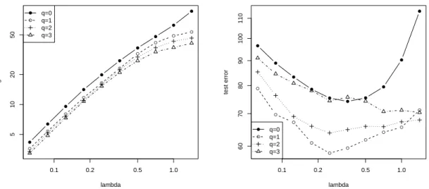
regularization where we do not penalize the features selected in the first stage. The procedure is described in Figure 1. Its overall effect is to “unshrink” coefficients of relevant features identified in the first stage. In practice, instead of tuningα, we may also let suppα( ˆβ) contain exactlyqelements, and simply tune the integer valued q. The parameters can then be tuned by cross validation in sequential order: first, find λ to optimize stage 1 prediction accuracy; second, find q to optimize stage 2 prediction accuracy. If cross-validation works well, then this tuning method ensures that the two-stage selective penalization procedure is never much worse than the one-stage procedure in practice because they are equivalent withq = 0. However, under right conditions, we can prove a much better bound for this two stage procedure, as shown in Theorem 8.1.
Tuning parameters: λ, α
Input: training data (x1,y1), . . . ,(xn,yn)
Output: parameter vector ˆβ0
• Stage 1: Compute ˆβ using (1).
• Stage 2: Solve the following selective penalization problem:
ˆ
β0 = arg min
β∈Rd
1
n
n
X
i=1
(βTxi−yi)2+λ
X
j /∈suppα( ˆβ) |βj|
.
Figure 1: Two-stageL1 Regularization with Selective Penalization
A related method, called relaxed Lasso, was proposed recently by Meinshausen [16], which is similar to a two-stage Dantzig selector in [4] (also see [12] for a more detailed study). Their idea differs from our proposal in that in the second stage, the parameter coefficientsβj0 are forced to be
zero whenj /∈supp0( ˆβ). It was pointed out in [16] that if supp0( ˆβ) can exactly identify all non-zero components of the target vector, then in the second stage, the relaxed Lasso can asymptotically remove the bias in the first stage Lasso. However, it is not clear what theoretical result can be stated when Lasso cannot exactly identify all relevant features. In the general case, it is not easy to ensure that relaxed Lasso does not degrade the performance when some relevant coefficients become zero in the first stage. On the contrary, the two-stage selective penalization procedure in Figure 1 does not require that all relevant features are identified. Consequently, we are able to prove a result for Figure 1 with no counterpart for relaxed Lasso. For clarity, the result is stated under similar conditions as those of the Dantzig selector in Theorem 6.1 with sparse targets andp= 2 only. Both restrictions can be easily removed with a more complicated version of Theorem 7.1 to deal with non-sparse targets (which can be easily obtained from Theorem 4.1) as well as the general form of Lemma 10.4 which allows p6= 2.
Theorem 8.1 Let Assumption 4.1 hold, and let Aˆ= n1Pn
i=1xixTi, and a= (supjAˆj,j)1/2.
Con-sider any target vector β¯ ∈ Rd such that Ey = ¯βTx, and β¯ contains only s non-zeros. Let k = |suppλ( ¯β)|. Consider the two-stage selective penalization procedure in Figure 1. Given δ ∈ (0,0.5), with probability larger than 1−2δ, for all (d−s)/2 ≥ ` ≥ s, and t ∈ (0,1). As-sume that
• t≤1−π(2)ˆ
A,k+`,`k
0.5/`.
• 0.5α≥λ≥4(2−t)t−1σap2 ln(2d/δ)/n. • either 16(αω(ˆp)
A,s+`)
−1s1/pλ ≤ t ≤ 1−π(p)
ˆ
A,s+`,`s
1−1/p/`, or 16(αµ(p)
ˆ
A,s+`)
−1(s+`)1/pλ ≤ t ≤
1−γ(ˆp)
A,s+`,`s
1−1/p/`.
Then
kβˆ0−β¯k2≤ 8
tµ(2)ˆ
A,k+`
h
5ρ(2)ˆ
A,k+`r
(2)
k ( ¯β) +
p
k−qλ+aσ(1 +p20 ln(1/δ))pq/ni+ 8rk(2)( ¯β),
where q =|supp1.5α( ¯β)|.
Again, we include a simplification of Theorem 8.1 under the mutual incoherence condition.
Corollary 8.1 Let Assumption 4.1 hold, and letAˆ= n1Pn
i=1xixTi , and assume thatAˆj,j= 1for all
j. DefineMAˆ= supi6=j|Aˆi,j|. Consider any target vectorβ¯such thatEy= ¯βTx, and assume thatβ¯
contains onlysnon-zeros wheres≤d/3and assume thatMAˆs≤1/6. Letk=|suppλ( ¯β)|. Consider
the two-stage selective penalization procedure in Figure 1. Givenδ∈(0,0.5), with probability larger
than 1−2δ: if α/48≥λ≥12σp2 ln(2d/δ)/n, then
kβˆ0−βk¯ 2≤24pk−qλ+ 24σ 1 +
r
20q
n ln(1/δ)
!
+ 168δk(2)( ¯β),
Theorem 8.1 can significantly improve the corresponding one-stage result (see Corollary 6.1 and Theorem 6.1) when r(2)k ( ¯β) √kλ and k −q k. The latter condition is true when
|supp1.5α( ¯β)| ≈ |suppλ( ¯β)|. In such case, we can identify most features in suppλ( ¯β). These con-ditions are satisfied when most non-zero coefficients in suppλ( ¯β) are relatively large in magnitude and the other coefficients are small (in 2-norm). That is, the two-stage procedure is superior when the target ¯β can be decomposed as a sparse vector with large coefficients plus another (less sparse) vector with small coefficients. In the extreme case when rk(2)(β) = 0 and q =k, we obtain
kβˆ0−βk¯ 2 =O(pkln(1/δ)/n) instead of kβˆ−β¯k2=O(pkln(d/δ)/n) for the one-stage Lasso. The difference can be significant whendis large.
Finally, we shall point out that the two-stage selective penalization procedure may be regarded as a two-step approximation to solving the least squares problem with a non-convex regularization:
ˆ
β0= arg min
β∈Rd
1
n
n
X
i=1
(βTxi−yi)2+λ d
X
j=1
min(α,|βj|)
.
However, for high dimensional problems, it not clear whether one can effectively find a good solution using such a non-convex regularization condition. When dis sufficiently large, one can often find a vector β such that|βj|> αand it perfectly fits (thus overfits) the data. This β is clearly a local minimum for this non-convex regularization condition since the regularization has no effect locally for such a vector β. Therefore the two-stage L1 approximation procedure in Figure 1 not only preserves desirable properties of convex programming, but also prevents such a local minimum to contaminate the final solution.
9
Experiments
Although our investigation is mainly theoretical, it is useful to verify whether the two stage proce-dure can improve the standard Lasso in practice. In the following, we show with a synthetic data and a real data that the two-stage procedure can be helpful. Although more comprehensive experi-ments are still required, these simple experiexperi-ments show that the two-stage method is useful at least on datasets with right properties — this is consistent with our theory. Note that instead of tuning the α parameter in Figure 1, in the following experiments, we tune the parameter q = suppα( ˆβ), which is more convenient. The standard Lasso corresponds toq = 0.
9.1 Simulation Data
In this experiment, we generate an n ×d random matrix with its column j corresponding to
[x1,j, . . . ,xn,j], and each element of the matrix is an independent standard Gaussian N(0,1). We
then normalize its columns so that Pn
i=1x2i,j = n. A truly sparse target ¯β, is generated with k
nonzero elements that are uniformly distributed from [−10,10]. The observation yi = ¯βTxi+i,
where each i ∼N(0, σ2). In this experiment, we take n= 25, d= 100, k = 5, σ = 1, and repeat
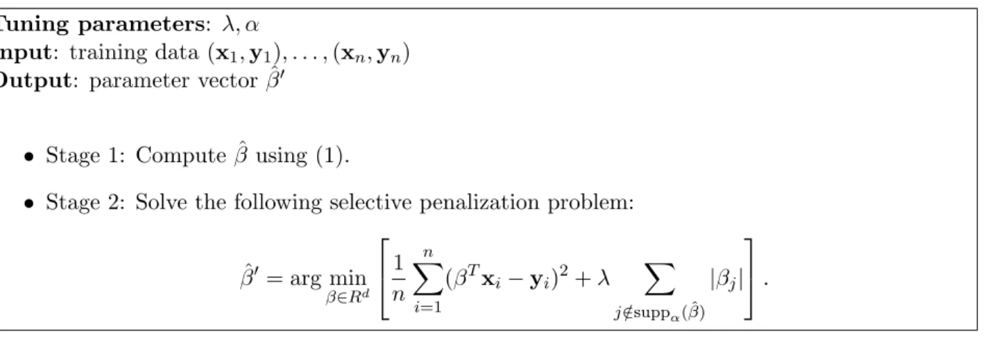
the experiment 100 times. The average training error and parameter estimation error in 2-norm are reported in Figure 2. We compare the performance of the two-stage method with different q
versus the regularization parameterλ. Clearly, the training error becomes smaller whenq increases. The smallest estimation error for this example is achieved atq= 3. This shows that the two-stage
procedure with appropriately chosenqperforms better than the standard Lasso (which corresponds toq= 0).
● ●
● ●
● ●
● ● ●
0.01 0.02 0.05 0.10 0.20 0.50 1.00 2.00
0.02
0.05
0.20
0.50
2.00
5.00
lambda
training error
● ●
● ●
● ●
●
● ● ●
●
q=0 q=1 q=3 q=5
● ●
● ● ●
●
● ● ●
0.01 0.02 0.05 0.10 0.20 0.50 1.00 2.00
2
3
4
5
6
7
lambda
parameter estimation error
● ●
● ●
● ●
●
● ● ●
●
q=0 q=1 q=3 q=5
Figure 2: Performance of the algorithms on simulation data. Left: average training squared error versusλ; Right: parameter estimation error versusλ.
9.2 Real Data
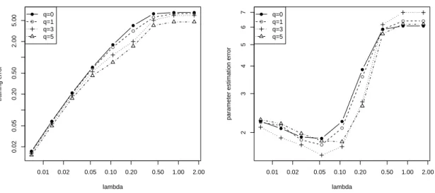
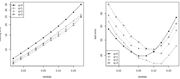
We use real data to illustrate the effectiveness of two-stage L1 regularization. For simplicity, we only report the performance on a single data, Boston Housing. This is the housing data for 506 census tracts of Boston from the 1970 census, available from theUCI Machine Learning Database Repository: http://archive.ics.uci.edu/ml/. Each census tract is a data-point, with 13 features (we add a constant offset on e as the 14th feature), and the desired output is the housing price. In the experiment, we randomly partition the data into 20 training plus 456 test points. We perform the experiments 100 times, and report training and test squared error versus the regularization parameter λ for different q. The results are plotted in Figure 3. In this case, q = 1 achieves the best performance. Note that this dataset contains only a small number (d= 14) features, which is not the case we are interested (most of other UCI data similarly contain only small number of features). In order to illustrate the advantage of the two-stage method more clearly, we also consider a modified Boston Housing data, where we append 20 random features (similar to the simulation experiments) to the original Boston Housing data, and rerun the experiments. The results are shown in Figure 4. As we can expect, the effect of using q > 0 becomes far more apparent. This again verifies that the two-stage method can be superior to the standard Lasso (q = 0) on some data.
● ●
● ●
● ●
● ●
● ●
0.02 0.05 0.10 0.20
10
15
20
25
30
35
lambda
training error
● ●
● ●
● ●
● ●
● ● ●
●
q=0 q=1 q=2 q=3
●
● ●
●
● ● ●
● ●
●
0.02 0.05 0.10 0.20
45
50
55
60
lambda
test error
●
● ●
● ●
●
● ● ●
● ●
●
q=0 q=1 q=2 q=3
Figure 3: Performance of the algorithms on the original Boston Housing data. Left: average training squared error versus λ; Right: test squared error versus λ.
10
Proofs
In the proof, we use the following convention: letI be a subset of{1, . . . , d}, and a vector β∈Rd, thenβI denotes either the restriction ofβ to indicesI which lies in R|I|, or its embedding into the
original space Rd, with components not inI set to zero.
10.1 Proof of Proposition 3.1
Given any v ∈ Rk and u ∈ R`, without loss of generality, we may assume that kvk2 = 1 and kuk2 = 1 in the following derivation. Take indices I and J as in the definition. We letI0 =I∪J.
Given anyα∈R, let u0T = [vT, αuT]∈R`+k. By definition, we have
µ(2)A,`+kku0k22 ≤u0TAI0,I0u0 =vTAI,Iv+ 2αvTAI,Ju+α2uTAJ,Ju.
Letb=vTAI,Ju,c1=vTAI,Iv, and c2 =uTAJ,Ju. The above inequality can be written as:
µ(2)A,`+k(1 +α2)≤c1+ 2αb+α2c2.
By optimizing over α, we obtain: (c1 −µ (2)
A,`+k)(c2 −µ (2)
A,`+k) ≥ b2. Therefore b2 ≤ (ρ
(2)
A,` −
µ(2)A,`+k)(ρ(2)A,k−µ(2)A,`+k), which implies that (with kvk2=kuk2 = 1)
vTA I,Ju
kvk2kuk∞
≤ |v
TA
I,Ju|
kvk2kuk2/√` ≤ √
`|b| ≤√`
q
(ρ(2)A,`−µ(2)A,`+k)(ρ(2)A,k−µ(2)A,`+k).
● ● ● ● ● ● ● ● ● ●
0.1 0.2 0.5 1.0
5 10 20 50 lambda training error ● ● ● ● ● ● ● ● ● ● ● ● q=0 q=1 q=2 q=3 ● ● ● ● ● ● ● ● ● ●
0.1 0.2 0.5 1.0
60 70 80 90 100 110 lambda
test error ●
● ● ● ● ● ● ● ● ● ● ● q=0 q=1 q=2 q=3
Figure 4: Performance of the algorithms on the modified Boston Housing data. Left: average training squared error versus λ; Right: test squared error versus λ.
The second inequality follows from kvkp≤kmax(0,1/p−0.5)kvk2 for all v∈Rk, so that kAI,Jukp
kuk∞
≤kmax(0,1/p−0.5)kAI,Juk2 kuk∞
.
From (c1−µ(2)A,`+k)(c2−µ(2)A,`+k)≥b2, we also obtain
4b2/c21 ≤4c−11(1−µ(2)A,`+k/c1)(c2−µ(2)A,`+k)≤(c2−µ(2)A,`+k)/µA,`(2)+k≤ρ(2)A,`/µ(2)A,`+k−1.
Note that in the above derivation, we have used 4µ(2)A,`+kc−11(1−µ(2)A,`+kc−11) ≤1. Therefore with
kvk2=kuk2 = 1:
vTAI,Jukvk2
vTA
I,Ivkuk∞
≤ |v
TA
I,Ju|
vTA I,Iv/
√
` =
|b| c1
√
`≤0.5`1/2
q
ρ(2)A,`/µ(2)A,`+k−1.
Because vand u are arbitrary, we obtain the third inequality.
The fourth inequality follows from max(0,vTAI,Ivp−1)≥ω(A,kp)kvkpp, so that
(vp−1)TA
I,Jukvkp
max(0,vTA
I,Ivp−1)kuk∞
≤ 1
ω(A,kp)
|(vp−1)TA I,Ju|
kvkpp−1kuk∞
≤ 1
ωA,k(p)
kAI,Jukp kuk∞
.
In the above derivation, the second inequality follows from k(v/kvkp)p−1kp/(p−1) = 1 and the
H¨older’s inequality.
The fifth inequality follows from kvkp ≤kmax(0,1/p−0.5)kvk
2 for all v∈Rk, so that kA−I,I1AI,Jukp
kuk∞
≤ kA
−1
I,IAI,Juk2
kuk∞
The sixth inequality follows from kA−I,I1vkp ≤ kvkp/µ(A,kp) for all v∈Rk, so that
kA−I,I1AI,Jukp
kuk∞
≤ 1
µ(A,kp)
kAI,Jukp
kuk∞
.
The last inequality is due to
kAI,Ivkp
kvkp =
k(v/kvkp)p−1kp/(p−1)kAI,Ivkp kvkp
≥(v
p−1)TA I,Iv
kvkpp
= (v
p−1)Tdiag(A I,I)v
kvkpp
+(v
p−1)T(A
I,I −diag(AI,I))v
kvkpp
≥min
i Ai,i− k(v/kvkp) p−1k
p/(p−1)
k(AI,I −diag(AI,I))vkp
kvkp
≥min
i Ai,i− kAI,I −diag(AI,I)kp.
In the above derivation, H¨older’s inequality is used to obtain the first two inequalities. The first equality and the last inequality use the fact thatk(v/kvkp)p−1kp/(p−1)= 1.
10.2 Proof of Proposition 3.2
Let B ∈ Rd×d be the off-diagonal part of A; that is, A−B is the identity matrix. We have supi,j|Bi,j| ≤MA. Given anyv∈Rk, we have
kBI,Ivkp≤MAk1/pkvk1 ≤MAkkvkp.
This implies thatkBI,Ikp ≤MAk. Therefore we have
kAI,Ivkp≤ kvkp(1 +M k).
This proves the first claim. Moreover,
(1−MAk)≤1− kBI,Ikp = min
i Ai,i− kAI,I−diag(AI,I)kp.
We thus obtain the second claim from Proposition 3.1. Now givenu∈R`, sinceI ∩J =∅, we have
kAI,Jukp =kBI,Jukp ≤MAk1/pkuk1 ≤MAk1/p`kuk∞.
This implies the third claim. The last two claims follow from Proposition 3.1.
10.3 Some Auxiliary Results
Lemma 10.1 Consider k, ` >0, and p∈ [1,∞]. Given any β,v∈ Rd. Let β = βF +βG, where
supp0(βF)∩supp0(βG) =∅ and |supp0(βF)|=k. Let J be the indices of the ` largest components
of βG (in absolute values), and I = supp0(βF)∪J. If supp0(v)⊂I, then
vTAβ≥vITAI,IβI− kAI,IvIkp/(p−1)γ (p)
A,k+`,`kβGk1`−1,
Proof In order to prove the first inequality, we may assume without loss of generality that
β = [β1, . . . , βd], where supp0(βF) = {1,2, . . . , k}, and when j > k, βj is arranged in descending
order of|βj|: |βk+1| ≥ |βk+2| · · · ≥ |βd|. LetJ0 ={1, . . . , k}, andJs ={k+ (s−1)`+ 1, . . . , k+s`}
(s= 1,2, . . .), except the largest index in the last block stops at d. Note that in this definition we
require that J1 =J and I = J0∪J1. We have kβJsk∞ ≤ kβJs−1k1`
−1 when s > 1, which implies
thatP
s>1kβJsk∞≤ kβGk1`
−1. This gives
vTAβ=vTIAI,IβI+
X
s>1
vITAI,JsβJs
≥vTIAI,IβI− kAI,IvIkp/(p−1)
X
s>1
kA−I,I1AI,JsβJskp ≥vTIAI,IβI−γA,(p|)I|,`kAI,IvIkp/(p−1)
X
s>1
kβJsk∞
≥vTIAI,IβI−γA,(p)|I|,`kAI,IvIkp/(p−1)kβGk1`−1.
The first inequality in the above derivation is due to the H¨older’s inequality. This proves the first inequality of the lemma.
The proof of the second inequality is similar, but with a slightly different estimate. We can assume that the right hand side is positive (the inequality is trivial otherwise). It implies that (vIp−1)TAI,IvI>0 since otherwiseωA,(p)|I|= 0:
(vp−1)TAβ=(vI(p−1))TAI,I(βI−vI) + (v(p
−1)
I )
TA
I,IvI+
X
s>1
(vpI−1)TAI,JsβJs
≥(v(Ip−1))TAI,I(βI−vI) + (v(p
−1)
I )
TA
I,IvI
"
1−π(A,p)|I|,`X
s>1
kβJsk∞/kvIkp
#
≥ −ρ(A,p)|I|kvI(p−1)kp/(p−1)kβI−vIkp+ (v(p
−1)
I )TAI,IvI
h
1−π(A,p)|I|,``−1kβGk1/kvIkp
i
≥ −ρ(A,p)|I|kvI(p−1)kp/(p−1)kβI−vIkp+ωA,(p)|I|kvIkpp
h
1−πA,(p)|I|,``−1kβGk1/kvIkp
i
.
The second inequality in the above derivation is due to the H¨older’s inequality. The last inequality assumes that the right hand side is non-negative. Observe that kvI(p−1)kp/(p−1) = kvIkpp−1, we
obtain the second inequality of the lemma.
Lemma 10.2 Consider the decomposition of any target vectorβ¯= ¯βF+ ¯βGsuch that{1,2, . . . , d}=
F ∪G and F ∩G= ∅. Consider the solution βˆ to the following more general problem instead of (1):
ˆ
β = arg min
β∈Rd
1
n
n
X
i=1
(βTxi−yi)2+λ
X
j /∈Fˆ
|βj|
, (5)
where Fˆ ⊂ F. Let ∆ ˆβ = ˆβ−β,¯ Aˆ = 1nPn
i=1xixTi , and ˆ= n1
Pn
i=1( ¯βTxi −yi)xi. If we pick a
sufficiently large λ in (5) such that λ >2kˆk∞, then
kβˆGk1 ≤
2kˆk∞+λ
λ−2kˆk∞
Proof We define the derivative of kβk1 as sgn(β), where for β = [β1, . . . , βd] ∈ Rd, sgn(β) =
[sgn(β1), . . . ,sgn(βd)]∈Rd is defined as sgn(βj) = 1 whenβj >0, sgn(βj) =−1 when βj <0, and
sgn(βj)∈[−1,1] when βj = 0. We start with the following first order condition:
2
n
n
X
i=1
( ˆβTxi−yi)xi+λg( ˆβ) = 0,
where g( ˆβ) = [g( ˆβ1), . . . , g( ˆβd)], with g( ˆβj) = 0 when j ∈Fˆ and g( ˆβj) = sgn( ˆβj) otherwise. This
implies that
2 ˆA∆ ˆβ+λg( ˆβ) =−2 n
n
X
i=1
( ¯βTxi−yi)xi.
Therefore, for all v∈Rd, we have
2vTAˆ∆ ˆβ≤ −2vTˆ−λvTg( ˆβ). (6) Now, letv= ∆ ˆβ in (6), and use the fact that ˆβGTg( ˆβG) = ˆβGTsgn( ˆβG) =kβˆGk1 as well askg( ˆβ)k∞≤
1, we obtain
0≤2∆ ˆβTAˆ∆ ˆβ ≤2|∆ ˆβTˆ| −λ∆ ˆβTg( ˆβ)
≤2k∆ ˆβk1kˆk∞−λ∆ ˆβF T
g( ˆβ)−λβˆGTg( ˆβ) +λβ¯GTg( ˆβ)
≤2(k∆ ˆβFk1+kβˆGk1+kβ¯Gk1)kˆk∞+λk∆ ˆβFk1−λkβˆGk1+λkβ¯Gk1
=(2kˆk∞−λ)kβˆGk1+ (2kˆk∞+λ)(k∆ ˆβFk1+kβ¯Gk1).
By rearranging the above inequality, we obtain the desired bound.
Lemma 10.3 Let the conditions of Lemma 10.2 hold. Let J be the indices of the largest ` coeffi-cients (in absolute value) of ∆ ˆβG, and I =F∪J. Ifλ≥4(2−t)t−1kˆk∞ for somet∈(0,1), then
∀p∈[1,∞],
k∆ ˆβk1≤4k1−1/pk∆ ˆβIkp+ 4kβ¯Gk1,
k∆ ˆβkp≤(1 + 3(k/`)1−1/p)k∆ ˆβIkp+ 4kβ¯Gk1`1/p−1.
Proof The condition onλimplies that (λ+ 2kˆk∞)/(λ−2kkˆ ∞)≤(4−t)/(4−3t)≤3. We have
from Lemma 10.2
k∆ ˆβGk1≤ kβ¯Gk1+kβˆGk1 ≤3k∆ ˆβFk1+ 4kβ¯Gk1.
Thereforek∆ ˆβ−∆ ˆβIk∞≤ k∆ ˆβGk1/`≤(3k∆ ˆβFk1+ 4kβ¯Gk1)/`, which implies that k∆ ˆβ−∆ ˆβIkp≤(k∆ ˆβGk1k∆ ˆβ−∆ ˆβIk∞p−1)1/p≤(3k∆ ˆβFk1+ 4kβ¯Gk1)`1/p−1.
Now, the first inequality in the proof also implies that
k∆ ˆβk1 ≤4k∆ ˆβFk1+ 4kβ¯Gk1.
By combining the previous two inequalities with k∆ ˆβFk1 ≤k1−1/pk∆ ˆβIkp, we obtain the desired