Available online through
ISSN 2229 – 5046
NEIGHBORHOOD DAKSHAYANI INDICES
V. R. KULLI*
Department of Mathematics, Gulbarga University, Gulbarga 585106, India.
(Received On: 11-06-19; Revised & Accepted On: 05-07-19)
ABSTRACT:
C
hemical Graph Theory is a branch of Mathematical Chemistry whose focus of interest is to finding graph invariantsof molecular graphs. These correlate with chemical properties of the chemical compounds. In this paper, we propose new degree based topological descriptors such as first and second neighborhood Dakshayani indices, vertex neighborhood Dakshayani index, first and second hyper neighborhood Dakshayani indices of a graph and establish explicit formulas for these indices of line graphs of subdivision graphs of certain nanostructures.
Key words: neighborhood Dakshayani indices, hyper neighborhood Dakshayani indices, nanostructures.
Mathematics Subject Classification: 05C07, 05C76, 92E10.
1. INTRODUCTION
Let G be a finite, simple connected graph with vertex set V(G) and edge set E(G). The degree dG(v) of a vertex v in G is
the number of edges incident to v. The set of all vertices which adjacent to v is called open neighborhood of v and denoted by NG (v). The closed neighborhood set of v is the set NG[v] = NG(v)∪{v}. The set NG[v] is the set of closed
neighborhood vertices of v. Let
(v)
(v)
G G G
u N
D
v
d
d
u
is the degree sum of closed neighborhood vertices ofv. The subdivision graph S(G) is the graph obtained from G by replacing each of its edge by a path of length 2. The line graph L(G) of G is the graph whose vertex set is E(G) and two vertices of L(G) are adjacent if they are adjacent in G. For other graph terminology and notation refer [1].
We need the following results.
Lemma 1: Let G be a (p, q) graph. Then S(G) has p+q vertices and 2q edges.
Lemma 2: Let G be a (p, q) graph. Then L(G) has q vertices and
( )
21
1
2
p
G i i
d
u
q
=
−
∑
edges.A molecular graph is a graph such that its vertices correspond to the atoms and the edges to the bonds. Chemical Graph Theory is a branch of Mathematical Chemistry which has an important effect on the development of the Chemical Sciences, Medical Sciences. A single number that can be used to characterize some property of the graph of a molecular is called a topological index for that graph. There are numerous topological indices that have found some applications in Chemistry, especially in QSPR/QSAR study, see [2, 3, 4]. Two of the best known and widely used topological indices are the first and second Zagreb indices by Gutman and Trinajstić [5]. Motivated by these definitions, we now introduce new degree based topological indices as follows:
The first neighborhood Dakshayani index is defined as
1
( )
.
G G
uv E G
ND G
D
u
D
v
The second neighborhood Dakshayani index is defined as
2
( )
.
G G
uv E G
ND G
D
u D
v
Corresponding Author: V. R. Kulli*
The vertex neighborhood Dakshayani index is defined as
2
( )
.
v G
u V G
ND G
D
u
Some results on Zagreb indices can be found in the papers [6, 7, 8].
The first hyper Zagreb index was introduced by Shirdel et al. in [9], defined as
2
1
( )
G G
uv E G
HM G
d
u
d
v
The second hyper Zagreb index was defined as [10]
2
2
( )
.
G G
uv E G
HM
G
d
u d
v
Some results on the hyper Zagreb indices can be found in the articles [11, 12].
Motivated by the above two definitions, we propose the following degree based topological indices:
The first hyper neighborhood Dakshayani index of a graph G is defined as
2
1
( )
.
G G
uv E G
HND G
D
u
D
v
The second hyper neighborhood Dakshayani index of a graph G is defined as
2
2
( )
G G
uv E G
HND G
D
u D
v
Recently, some hyper indices like hyper Revan indices [13], reverse hyper Zagreb indices [14], K hyper Banhatti indices [15] were introduced and studied.
Recently, the first neighborhood Zagreb index was introduced and studied by Basavanagoud et al. [16] and Mondal
et al. [17].
We consider 2D-lattice, nanotube and nanotorus of TUC4C8 [p, q], see [18, 19]. In this paper, we determine the first and
second neighborhood Dakshayani indices, the vertex neighborhood Dakshayani index, first and second hyper neighborhood Dakshayani indices of line graphs of subdivision graphs of 2D-lattice, nanotube and nanotorus of
TUC4C8 [p, q].
2. 2-D LATTICE, NANOTUBE AND NANOTORUS OF TUC4C8 [p, q]
In this section, we consider the graph of 2D-lattice, nanotube and nanotorus of TUC4C8 [p, q], where p is the number of
squares in a row and q is the number of rows of squares. These graphs are depicted in Figure 1.
(a) (b) (c)
Figure-1
(a) 2D-lattice of TUC4C8[4, 2] (b) TUC4C8[4,2] nanotube (c) TUC4C8 [4, 2] nanotorus 3. RESULTS FOR 2D-LATTICE OF TUC4C8 [p, q]
The line graph of the subdivision graph of 2D-lattice of TUC4C8 [p, q] is presented in Figure 2(b).
(a) (b)
subdivision graph of line graph of the subdivision 2D-lattice of TUC4C8[4,2] graph of TUC4C8 [4, 2]
Theorem 1: Let G be the line graph of the subdivision graph of 2D-lattice of TUC4C8 [p, q]. Then the first
neighborhood Dakshayani index of G is given by
ND1(G) = 432pq – 628(p+q) + 8, if p > 1, q > 1,
= 260p – 164, if p > 1, q = 1.
Proof: The 2D-lattice of TUC4C8[p, q] is a graph with 4pq vertices and 6pq – p – q edges. By Lemma 1, the
subdivision graph of 2D lattice of TUC4C8[p, q] is a graph with 10pq – p – q vertices and 2(6pq – p – q) edges. Hence
by Lemma 2, G has 2(6pq – p – q) vertices and 18pq – 5p – 5q edges. Clearly, the vertices of G are either of degree 2 or 3, see Figure 2(b). Thus the edge partition of G is given in Table 1 and Table 2.
DG(u), DG(v)\ uv ∈E(G) (6, 6) (6,7) (7, 7) (7, 11) (11, 12) (12, 12)
Number of edges 4 8 2(p+q – 4) 4(p+q – 2) 8(p+q – 2) 2(9pq+10) – 19(p+q)
Table-1: Edge partition of G with p > 1, q >1
DG(u), DG(v)\ uv ∈E(G) (6, 6) (6,7) (7, 7) (7, 11) (11, 11) (11, 12) (12, 12)
Number of edges 6 4 2(p – 2) 4(p – 1) 2(p – 1) 4(p – 1) (p – 1)
Table-2: Edge partition of G with p > 1 and q = 1
Case-1: Let p >1 and q > 1.
The edge partition based on the degree sum of closed neighborhood vertices of each vertex is obtained, as given in Table 1. To compute ND1(G), we see that
1
( )
G G
uv E G
ND G
D
u
D
v
4 6
6
8 6
7
2
p
q
4 7
7
4
p
q
2
7
11
8
p
q
2 11 12
2 9
pq
10
19
p
q
12
12
432
628
8.
pq
p
q
Case-2: Let p > 1 and q = 1.
The edge partition based on the degree sum of closed neighborhood vertices of each vertex is obtained, as given in Table 2. To compute ND1(G), we see that
1
( )
G G
uv E G
ND G
D
u
D
v
6 6
6
4 6
7
2
p
2 7
7
4
p
1
7
11
2
1 11 11
4
1 11 12
1 12
12
p
p
p
260
164.
p
Theorem 2: Let G be the line graph of the subdivision graph of 2D-lattice of TUC4C8[p, q]. Then the second
neighborhood Dakshayani index of G is given by
ND2(G) = 2592pq – 4010(p+q) + 436, if p > 1, q > 1,
= 1586pq – 1202, if p > 1, q = 1.
Proof:
Case-1: Let p > 1 and q >1.
The edge partition based on the degree sum of closed neighborhood vertices of each vertex is obtained, as given in table 1. To compute ND2(G), we see that
2
( )
G G
uv E G
ND G
D
u D
v
4 6 6
8 6 7
2
p
q
4 7 7
4
p
q
2
7 11
8
p
q
2 11 12
2 9
pq
10
19
p
q
12 12
2592
4010
436.
pq
p
q
Case-2: Let p > 1 and q = 1.
To compute ND2(G), we see that
2
( )
G G
uv E G
ND G
D
u D
v
6 6 6
4 6 7
2
p
2 7 7
4
p
1
7 11
2
1 11 11
4
1 11 12
1 12 12
p
p
p
1586
1202.
p
Theorem-3: Let G be the line graph of the subdivision graph of 2D-lattice of TUC4C8 [p, q]. Then the first hyper
neighborhood Dakshayani index of G is given by
HND1(G) = 10368pq – 5024(p+q) + 1608, if p > 1, q > 1,
= 5348p – 4200, if p > 1, q = 1.
Proof:
Case-1: Let p > 1 and q > 1.
The edge partition based on the degree sum of closed neighborhood vertices of each vertex is obtained, as given in Table 1.
To compute HND1(G), we see that
2
1
( )
G G
uv E G
HND G
D
u
D
v
2
2
4 6
6
8 6
7
2
p
q
4
27
7
4
p
q
2
7
11
2
8
p
q
2 11
12
2
2 9
pq
10
19
p
q
12
12
2
10368
pq
5024
p
q
1608.
Case-2: Let p>1 and q = 1.
The edge partition based on the degree sum of closed neighborhood vertices of each vertex is obtained, as given in Table 2. To compute HND1(G), we see that
2
1
( )
G G
uv E G
HND G
D
u
D
v
6 6
6
2
4 6
7
2
2
p
2 7
7
2
4
p
1 7
11
2
2
p
1 11 11
2
4
p
1 11 12
2
2
p
1 12
12
2
5348
p
4200.
Theorem 4: Let G be the line graph of the subdivision graph of 2D-lattice of TUC4C8 [p, q]. Then the second hyper
neighborhood Dakshayani index of G is given by
HND2(G) = 374248pq – 226074(p+q) + 106116, if p > 1, q > 1,
= 148232p – 138202, if p > 1, q = 1.
Proof:
Case-1: Let p >1 and q >1.
The edge partition based on the degree sum of closed neighborhood vertices of each vertex is obtained as given in Table 1.
To compute HND2(G), we see that
2
2
( )
G G
uv E G
HND G
D
u D
v
2 2
24 6 6
8 6 7
2
p
q
4 7 7
4
p
q
2
7 11
2
28
p
q
2 11 12
2 9
pq
10
19
p
q
12 12
2
374248
p
226074
p
q
106116.
Case-2: Let p >1 and q = 1.
To compute HND2(G), we see that
2
2
( )
G G
uv E G
HND G
D
u D
v
2 2
6 6 6
4 6 7
22
p
2 7 7
4
p
1
7 11
2
22
p
1 11 11
24
p
1 11 12
p
1
12 12
2
148232
p
138202.
Theorem-5: Let G be the line graph of the subdivision graph of 2D-lattice of TUC4C8 [p, q]. Then the vertex
neighborhood Dakshayani index of G is
NDv(G) = 1728pq – 760(p+q) + 80, if p > 1, q > 1,
= 968p – 680, if p > 1, q = 1.
Proof: In Theorem 1, it is known that G has 2 (6pq – p – q) vertices. The vertex partition based on the degree sum of closed neighborhood vertices of each vertex is obtained, as given in Table 3 and Table 4.
DG(u) \ u ∈V(G) 6 7 11 12
Number of vertices 8 4 (p+q – 2) 4 (p+q – 2) 2(6pq – 5p – 5q + 4)
Table-3: Vertex partition of G with p>1 and q > 1
DG(u) \ u ∈V(G) 6 7 11 12
Number of vertices 8 4 (p – 1) 4 (p – 1) 2(p – 1)
Table-4: Vertex partition of G with p >1 and q = 1
Case-1: Let p >1 and q > 1.
By using the definition and Table 3, we deduce
2
( )
v G
u V G
ND G
D
u
2 2
8 6
4
p
q
2 7
4
p
q
2 11
2
2 6
pq
5
p
5
q
4 12
2
1728
pq
760
p
q
80.
Case-2: Let p > 1 and q = 1.
By using the definition and Table 4, we derive
2
( )
v G
u V G
ND G
D
u
2 2
8 6
4
p
1 7
24
p
1 11
2
p
1 12
2968
p
680.
4. RESULTS FOR TUC4C8 [p, q] NANOTUBE
The line graph of the subdivision graph of TUC4C8 [p, q] nanotube is presented in Figure 3 (b).
(a) (b)
Subdivision graph Line graph of subdivision of TUC4C8[4, 2] nanotube graph of TUC4C8[4, 2]
Theorem 6: Let H be the line graph of the subdivision graph of TUC4C8[p, q] nanotube. Then the first neighborhood
Dakshayani index of H is
ND1(H) = 432pq – 172p, if p > 1, q > 1,
= 260p, if p > 1, q = 1.
Proof: The TUC4C8[p, q] nanotube is a graph with 4pq vertices and 6 pq – p edges. By Lemma 1, the subdivision graph
of TUC4C8[p, q] nanotube is a graph with 10pq – p vertices and 12pq – 2p edges. Therefore by Lemma 2, H has
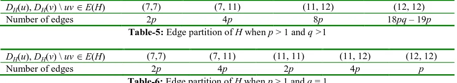
12pq – 2p vertices and 18pq – 5p edges. Clearly the vertices of H are either of degree 2 or 3, see Figure 3 (b). Thus the partition of the edge set of H is as shown in Table 5 and Table 6.
DH(u), DH(v) \ uv∈E(H) (7,7) (7, 11) (11, 12) (12, 12)
Number of edges 2p 4p 8p 18pq – 19p
Table-5: Edge partition of H when p > 1 and q >1
DH(u), DH(v) \ uv∈E(H) (7,7) (7, 11) (11, 11) (11, 12) (12, 12)
Number of edges 2p 4p 2p 4p p
Table-6: Edge partition of H when p > 1 and q = 1
Case-1: Let p > 1 and q > 1.
The edge partition based on the degree sum of closed neighborhood vertices of each vertex is given in Table 5.
To compute ND1(H), we see that
1
( )
H H
uv E H
ND H
D
u
D
v
2
p
7
7
4
p
7
11
8
p
11 12
18
pq
19
p
12
12
432
pq
172 .
p
Case-2: Let p > 1 and q = 1.
The edge partition based on the degree sum of closed neighborhood vertices of each vertex is obtained, as given in Table 6.
By using definition and Table 6, we deduce
1
( )
H H
uv E H
ND H
D
u
D
v
2
p
7
7
4
p
7
11
2
p
11
11
4 (11
p
12)
p
12
12
260 .
p
Theorem 7: Let H be the line graph of the subdivision graph of TUC4C8[p, q] nanotube. Then the second neighborhood
Dakshayani index of H is
ND2(H) = 2592pq – 1274p, if p > 1, q > 1,
= 1320p, if p > 1, q = 1.
Proof: Case 1. Let p > 1 and q > 1.
The edge partition based on the degree sum of closed neighborhood vertices of each vertex is given in Table 5.
By using definition and Table 5, we obtain
2
(H)
H H
uv E
ND
H
D
u D
v
2
p
7 7
4
p
7 11
8
p
11 12
18
pq
19
p
12 12
1592
pq
1274 .
p
Case-2: Let p > 1 and q = 1.
By using definition and Table 6, we derive
2
( )
H H
uv E H
ND H
D
u D
v
2
p
7 7
4
p
7 11
2
p
11 11
4
p
11 12
p
12 12
1320 .
p
Theorem 8: Let H be the line graph of the subdivision graph of TUC4C8 [p, q] nanotube. Then the first hyper
neighborhood Dakshayani indices of H is
HND1(H) = 10368pq – 4424p, if p > 1, q > 1,
= 5348p, if p > 1, q = 1.
Proof: Case 1. Let p >1, q > 1.
The edge partition based on the degree sum of closed neighborhood vertices of each vertex is given in Table 5.
By using definition and Table 5, we obtain
2
1
( )
H H
uv E H
HND H
D
u
D
v
2
2
2
22
p
7
7
4
p
7
11
8
p
11 12
18
pq
19
p
12
12
10368
pq
4424 .
p
Case-2: Let p > 1 and q = 1.
The edge partition based on the degree sum of closed neighborhood vertices of each vertex is obtained, as given in Table 6.
To compute HND1(H), we see that
2
1 H H
uv E H
HND H
D
u
D
v
2
2
2
2
22
p
7
7
4
p
7
11
2
p
11 11
4
p
11 12
p
12
12
5348 .
p
Theorem 9: Let H be the line graph of the subdivision graph of TUC4C8 [p, q] nanotube. Then the second hyper
neighborhood Dakshayani index of H is
HND2(H) = 373248pq – 226074p, if p > 1, q > 1,
= 148232p, if p > 1, q = 1.
Proof:Case 1. Suppose p > 1, q > 1.
The edge partition based on the degree sum of closed neighborhood vertex of each vertex is given in Table 5.
By using definition and Table 5, we have
2
2
( )
H H
uv E H
HND H
D
u D
v
2 2 2
22
p
7 7
4
p
7 11
8
p
11 12
18
pq
19
p
12 12
373248
pq
226074 .
p
Case-2: Suppose p > 1, q = 1.
The edge partition based on the degree sum of closed neighborhood vertex of each vertex is obtained as given in Table 6.
By using definition and Table 6, we obtain
2
2
( )
H H
uv E H
HND H
D
u D
v
2 2 2 2 2
2
p
7 7
4
p
7 11
2
p
11 11
4
p
11 12
p
12 12
148232 .
p
Theorem 10: Let H be the line graph of the subdivision graph of TUC4C8 [p, q] nanotube. Then the vertex
neighborhood Dakshayani index of H is
NDv(H) = 1728pq – 760p, if p > 1 , q > 1,
= 968p, if p >1, q = 1.
Proof: In Theorem 6, it is known that H has 12pq – 2p vertices. The vertex partition based on the degree sum of closed neighborhood vertices of each vertex is given in Table 7 and Table 8.
DH(u) \ u∈V(H) 7 11 12
Number of vertices 4p 4p 12pq – 10p
Table-7: Vertex partition of H when p >1, q > 1
DH(u) \ u∈V(H) 7 11 12
Number of vertices 4p 4p 2p
Table-8: Vertex partition of H when p > 1, q = 1
Case-1:. Let p >1 and q > 1.
By using the definition and Table 7, we derive
2
v H
u V H
ND H
D
u
2 2 2
4
p
7
4
p
11
12
pq
10
p
12
1728
pq
760 .
p
Case-2: Let p >1 and q = 1.
From the definition and by using Table 8, we deduce
2
v H
u V H
ND H
D
u
2 2 2
4
p
7
4
p
11
2
p
12
968 .
p
5. RESULTS FOR TUC4C8 [p, q] NANOTORUS
The line of the subdivision graph of TUC4C8[p, q] nanotorus is shown in Figure 4(b).
(a) (b)
Subdivision graph of Line graph of subdivision
TUC4C8[p, q] nanotorus graph of TUC4C8[p, q] nanotorus Figure-4
Theorem 11: Let K be the line graph of the subdivision graph of TUC4C8 [p, q] nanotorus. Then
ND1(K) = 432pq.
ND2(K) = 2592pq.
HND1(K) = 10368pq.
HND2(K) = 373248pq.
N1*(K) = 1728pq.
Proof: A graph of TUC4C8[p, q] nanotorus has 4pq vertices and 6pq edges. By Lemma 1, the subdivision graph of
TUC4C8 [p, q] nanotorus is a graph with 10pq vertices and 12pq edges. Hence by Lemma 2, K has 12pq vertices and
18pq edges. Clearly the degree of each vertex is 3. The edge partition based on the degree sum of closed neighborhood vertices of each vertex is as given in Table 9.
DK(u), DK(v)\ uv ∈E(K) (12, 12)
Number of edges 18pq
By using definitions and Table 9, we have
1 K K
18
12
12
432
.
uv E K
ND K
D
u
D
v
pq
pq
2 K K
18
12 12
2592
.
uv E K
ND K
D
u D
v
pq
pq
2 2
1 K K
18
12
12
10368
.
uv E K
HND K
D
u
D
v
pq
pq
2 2
2 K K
18
12 12
373248
.
uv E K
HND K
D
u D
v
pq
pq
The vertex partition based on the degree sum of closed neighborhood vertices of each vertex is as given in Table 10.
DK(u)/ u ∈V(K) 12
Number of vertices 12pq
Table-10: Vertex partition of K
From definition and using Table 10, we obtain
2 2
12
12
1728
.
v K
u V K
ND K
D
u
pq
pq
REFERENCES
1.
V.R. Kulli, College Graph Theory, Vishwa International Publications, Gulbarga, India (2012).2.
I. Gutman and O.E. Polansky, Mathematical Concepts in Organic Chemistry, Springer, Berlin (1986).3.
V.R. Kulli, Multiplicative Connectivity Indices of Nanostructures, LAP LEMBERT Academic Publishing (2018).4.
R. Todeschini and V. Consonni, Molecular Descriptors for Chemoinformatics, Wiley-VCH, Weinheim, (2009).5.
I. Gutman and N. Trinajstić, Graph theory and molecular orbitals. Total π-electron energy of alternant hydrocarbons, Chem. Phys. Lett. 17 (1972) 535-538.6.
K.C. Das and I. Gutman, Some properties of the second Zagreb index, MATCH Commun. Math. Comput.Chem. 52 (2004) 103-112.
7.
I. Gutman, B. Furtula, Z. K. Vukićević and G. Popivoda, On Zagreb indices and coindices, MATCH Commun.Math. Comput. Chem. 74 (2015) 5-16.
8.
S. Nikolić, G. Kovaćević, A. Milićević and N. Trinajstić, The Zagreb indices 30 years after, Croatica ChemicaActa CCACAA 76(2) (2003) 113-124.
9.
G.H. Shirdel, H. Rezapour and A.M. Sayadi, The hyper-Zagreb index of graph operations, Iranian J. Math. Chem. 4(2) (2013) 213-220.10.
W. Gao, M.R. Farahari, M. K. Siddiqui, M. K. Jamil, On the first and second Zagreb and first and second
hyper Zagreb indices of carbon nanocones CNCk[n], J. Comput. Theor. Nanosci. 13 (2016) 7475-7482.11.
F. Falahati Nezhad, M. Azari, Bounds on the hyper Zagreb index,
J. Appl. Math. Inform. 34 (2016) 319-330.12.
B. Basavanagoud and S. Patil, A note on hyper Zagreb index of graph operation,
Indian J. Math. Chem. 7(1) (2016) 89-92.13.
V.R. Kulli, Hyper Revan indices and their polynomials of silicate networks,
International Journal of CurrentResearch in Science and Technology, 4(3) (2018) 17-21.
14.
V.R. Kulli, Reverse Zagreb and reverse hyper-Zagreb indices and their polynomials of rhombus silicate
networks, Annals of Pure and Applied Mathematics, 16(1) (2018) 47-51.15.
V.R. Kulli, On
K hyper-Banhatti indices and coindices of graphs, Journal of Computer and MathematicalSciences, 6(5) (2016) 300-304.
16.
B. Basavanagoud, A. P. Barangi and S. M. Hosamani, First neighbourhood Zagreb index of some
nanostructures, Proceedings IAM. 7(2) (2018) 178-193.17.
S. Mondal, N. De, A. Pal, On neighbourhood index of product of graphs, arXivi1805.05273v1 [math.Co] 14
May 2018.18.
S. M. Hosamani, Computing Sanskruti index of certain nanostructures,
J. Appl. Math. Comput. 54(1-2) (2017) 425-433.19.
V.R. Kulli, New multiplicative arithmetic-geometric indices,
Journal of Ultra Scientist of Physical Sciences, A, 29(6) (2017) 205-211.Source of support: Nil, Conflict of interest: None Declared.