JEEECCS, Volume 1, Issue 2, pages 31-36, 2015
Numerical And Experimental Aspects
Concerning The Static and Dynamic Regime
Of A Linear Actuator
Constantin Stoica, Dumitru Cazacu,1Ion Catalin2
1
Dept. of electronics, computers and electrical engineering
University of Pitesti, Romania
2
Graduated at Electrical Engineering, Univ.Pitesti
Leonard Melcescu
Department of electrical Machines
University “Politehnica” Bucharest Bucharest, Romania
Abstract – In this paper the dynamic behavior of a D.C. linear actuator is analyzed. A finite element numerical model was used. A coupled system of electrical and mechanical differential equations was solved by coupled simulation among magnetic field transitory regime, electric circuit and mechanical translation with variable speed. The time variations of the current, of the magnetic force and of the moving part speed were determined. The current variation was validated by experimental measurements.
Keywords- linear actuator;dynamic regime; finite element method;coupled problem
I. INTRODUCTION
Linear actuators have many applications in digitally controlled compact pumps, electromagnetic valves, circuit breakers, micro machines and robotics. In order to simulate the dynamic behavior of a linear actuator a coupled problem that comprises magnetic field, electrical circuit and mechanical motion, has to be solved.
In [1] certain finite element numerical models of electro mechanical systems are presented. In [2] the basics of the switching equipments are presented. Paper [3] deals with a linear actuator that has an axially magnetized moving magnet. Paper [4] focuses on modeling and simulation of the electromagnetic actuators integrated in ABB’s reclosers. Paper [5] presents an accurate model for optimization of design and supply control for linear actuators.
In [6-8] the application of finite element method to actuators study is presented. In the literature there are coupled and decoupled approaches. The decoupled solves the problems sequentially: magneto-static, electric circuit and mechanical movement.
In [9] a decoupled dynamic model that employs bi-cubic spline approximations of the results from the magnetostatic field analysis and compare it with the
coupled model. In the coupled approach [10], all the problems should be solved simultaneously. In this paper the analysis of the dynamic behavior of a D.C. linear actuator is performed by finite method. It is a coupled simulation among magnetic field transitory regime, electric circuit and mechanical translation with variable speed.
The numerical model was validated by experimental measurements.
II. THEORETICALASPECTS
A. Mathematical model
In order to determine the time variations of the moving part speed v(t), of the current i(t) and of the magnetic force Fm(t) the following system of coupled electromagnetic, electric circuit and mechanical motion equations have to solved, considering that the movement is performed along the Oz axis [ 9] :
- the electromagnetic field equation
0 ) ( )
( 0
v B M
t A J
A e
(1)
where
A
is the magnetic vector potential having only the azimuthally componentA
,
is themagnetic reluctivity,
J
eis the current density in thecoil,
is the electric conductivity,v
is the velocity of the plunger,B
is the magnetic flux density,
0 is the magnetic permeability for thefree space and
M
is the magnetization vector- the electric circuit equation :
v
dz
z
dL
i
dt
di
z
L
i
R
where
U
0is the supply voltage, R is the resistanceof the coil, L is the variable inductivity of the coil i
is the electric current and z is the discrete value of
the air gap
.- the mechanical motion equation :
r load
m
F
F
F
a
m
(3)where
F
mis the magnetic force,F
loadis the load force andF
r
x
is another resistant force that can depend on the speed .To calculate the force exerted on the plunger, the Maxwell stresses or the virtual work method can be used.
The volume density of the magnetic force
f
Vm , within a certain volume VΣ can be reduced to a system of fictitious stresses acting on the surface Σ that bounds the considered volume.Equivalent condition is that the resultant force must be the same:
dA
T
dV
f
F
nV Vm
m
(4)
where Tn is magnetic Maxwell stress tensor.
The virtual work method for computing force and torques is derived from magnetic energy Wm or co energy Wm’ changes against space displacement.
The magnetic force Fm is obtained from the generalized magnetic force theorem, when the current is constant:
.
)
(
m i ctm
z
W
F
(5)Rewriting equation (3), using (5) we obtain equation (6) that describes the motion of the plunger:
z
F
F
dz
z
dL
i
dt
z
d
m
(
)
load
r2
1
2 2 2(6)
In the case of high magnetic permeability (ferromagnetic material), a simplified expression for the force can be obtained [11]:
2 0 2 2
0
2
1
N
I
A
F
(7)From relation (6), some observations can be drawn: - the magnetic force is directly proportional to cross section of the plunger;
- force is reverse proportional to the square air gap length, and it tends to reduce the air gap;
- being an attraction force between two magnetic parts, the mobile and fixed ones, a steady state is
obtained only for a minimum value of magnetic energy.
III. NUMERICAL SIMULATIONS
Numerical calculation of the magnetic field was done using Flux 2D software package developed by the Cedrat company.
A dc linear actuator (with plunger), produced by INTERTEC Components GmbH, was studied. It has the following characteristics: power supply 12 V dc, number of turns N = 288 and the connection current I=0.33 A.
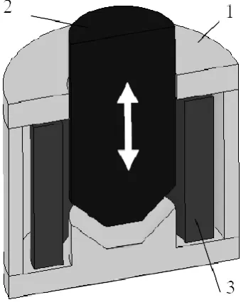
In this electromagnet with limiter type, the air gap is between two truncated cone surfaces, and the force exerted is pulling.
Figure 1. The studied linear actuator
A. The geometry
The axial cross section through the electromagnet is described in Fig., where 1 is the fixed part (the case), 2 is the plunger (made of massive steel) and 3 is the coil.
Figure 2. Axial cross section in the dc actuator
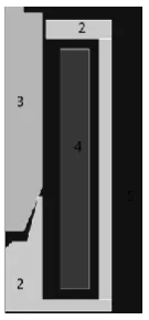
The geometry dimensions of the actuator are presented in Fig.3
Figure 3. The model geometry
The elements of the geometry are : 2 is the case, 3 is the plunger, 4 is the coil and 5 is the aer (Fig.4)
Figure 4. Model components
B. The material properties
The non linear characteristic B (H) of the steel from the plunger has the saturation flux density Bs=1.9 T and the initial relative magnetic permeability is
ri
500
. It is represented in Fig.5.The other regions of the field domain are non magnetized. The steel electrical resistivity is 0.2106mFigure 5. The B-H characteristic of the steel used for the plunger
C. The mesh
The mesh is composed of triangular finite elements and the areas of the translating region are devised in rectangles.
On the width of the translation strip there is only one triangular finite element .The mesh had 149285 nodes. (Fig.6)
Figure 6. The mesh of the actuator
The mesh is concentrated in the plunger , in the coil and in the airgap .In Fig 7 the general mesh of the whole field domain is presented.
Figure 7. The whole mesh
The external light blue mesh area is a special region used to model problem with infinit boundary, by default non conductive and non magnetic.
D. The boundary conditions
The limit of the computation domain (which is the also the axis of the actuator) is a magnetic field line, where the Dirichlet boundary condition is imposed (the magnetic vector potential (MVP) A = 0).
The external light blue area indicates also that the magnetic field vanishes at infinity.
E. Anslysis and results
Being a 2D axial symmetric model the electromagnet presents a rotation symmetry described by the cylindrical system of coordinates (r, φ, and z).
As a consequence the transitory regime is described by a time variable current source J (t) and a MVP A, time and space dependent.
The equation of the field model is:
J
t
A
A
rot
rot
)
(
)]
/
1
[(
(8)where ρ is the electric resistivity and μ is the magnetic permeability.
The second term from the left hand side of the equation represents the density of the induced currents, which is non zero in the conducting regions.
In Fig.8 the equipotential lines of the magnetic field are represented.
t = 10 ms
Figure 8. The equipotential lines distribution
In Fig.9 the flux density distribution is presented.
t = 10 ms
Figure 9. The flux density distribution
F. The coupled analysis
The 2D Transient Magnetic application is used. In order to describe the equivalent electric circuit of the electromagnet the Circuit Editor function has been used.
The simulated electric circuit is presented in Fig.10. It comprises the actuator coil inductivity, a dc power supply and an electric resistance of 0.1 Ohm, used for measurements.
Figure 10. The electric circuit model of the actuator
The equation 7 is solved in time domain, step by step. The current source from this equation is initially unknown.
At any moment of time the current density J has a constant but unknown value. A certain link between the MVP and J is assured by the circuit model of the application.
The step by step method is used because a part of the computation field domain, the moving part, changes the position in time.
The non linear algebraic system of equations obtained by finite element method was solved by Newton Raphson method.
The transitory regime of the electric current from coil is dependent on its resistance R and inductivity L.
The inductivity L is time variable because of the moving part. In Fig.11 the time variation of the current is presented.
Figure 11. Coil current vs time
Three stages can be noticed.
The first one begins when we supply the electromagnet until the moment the plunger starts moving. In this stage the variation of the coil inductance is small and the current increases exponentially.
The second stage begins when the moving part begins to move, from the initial value of the air gap 6mm to the final value 0.5 mm. At the beginning the inductivity varies slowly but at the end of the interval the growing up is explosive such as, due to the self induction voltage, the absorbed current goes down, after it reaches a maximum value.
slower that in the first stage, because the coil inductance is greater.
In order to evaluate de simulation time and the time steps the problem was first solved in magneto static regime for the total current.
Two magneto static problems were solved, each one corresponding to the initial and to the final value of the air gap, respectively.
The time variation of the magnetic force is presented in Fig.12
Figure 12. Magnetic force vs.time
It can be noticed that the force decreases as the air gap grows. This variation depends on the geometry of the plunger (the skewing angle) and on the material used.
The time variation of the plunger speed is presented in Fig.13.
Figure 13. Plunger speed vs time
It can be noticed that the speed of the plunger increases rapidly until it reaches the end of the course and than instantaneously drops to zero at the end.
G. Experimental validation of the numerical
model
The main elements of the experimental equipment are the variable voltage source Hameg and the electronic oscilloscope Scopix 7204 Metrix. In order to measure the time variation of the current a resistance of 0.1 ohm was connected with the actuator. The information obtained, the fast variable signal in Fig.14, was filtered and represented as the thicker curve in same figure.
Figure 14. The current vs. time
A good agreement between the measured and the computed current time variation can be noticed. The stable value of the current 0.35 A is amost the same in both cases.Also the time interval to reach that value is about 10 ms in both cases.
The time for the minimum value of the current is about 20 ms for numerical model and about 23 ms for the experimental one.
In order to determine the actuator force an electronic scale was used (Fig.15). The plunger was connected to it with a slide rod.
The actuator was mounted on a slide fixed on the slide rod. The movement of the slide is performed by a step by step motor that allows a good adjustment .
Figure 15. The experimental measuring equipement
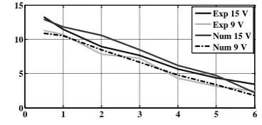
In Fig.16 the experimental and the numerical static characteristic of the actuator for 9 V and 15 V are considered.
0 1 2 3 4 5 6
0 5 10 15
Exp 15 V Exp 9 V Num 15 V Num 9 V
Figure 16. Numerical vs experimental static characteristics at different voltages
The third and the forth upper curves (from the top) represents the numerical and the experimental static characteristic, respectively, at 9 V.
The magnetic forces have greater values as the voltage increases. It can be noticed that as the air gap increases the differences between the measured and the calculated values grow up.
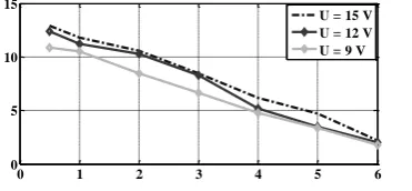
In Fig.17 experimental static characteristics at different voltages are compared.
From the top ,the first curve is at 15 V, the line dot curve is at 12 V and the last one is at 9 V.
0 1 2 3 4 5 6
0 5 10 15
U = 15 V U = 12 V U = 9 V
Figure 17. Experimental static characteristics at different voltages
In Fig.18 numerical static characteristics at different voltages are compared.From the top, the line dot curve is at 15 V, the second one is at 12 V and the third one is at 9 V.
0 1 2 3 4 5 6
0 5 10 15
U = 15 V U = 12 V U = 9 V
Figure 18. Numerical static characteristics at different voltages
In both figures 16 and 17 we can observe that the magnetic forces are mostly higher when the voltage increses.
IV. CONCLUSIONS
In this paper numerical (static and dynamic) simulations and experimental measurements of a linear actuator were performed.The static analysis was performed at different voltages : 9V, 12 V and 15 V.
It is a good agreement between the numerical and the experimental characteristics.
The differences between the experimental and numerical static characteristics are caused by the difference between the real B(H) characteristics and the used one.
The numerical time variation of the transitory current meets closely the experimental result. Future work will analyse the influence of different ferromagnetic materials for the plunger on the duration of the transitory regime as well the influence of a plunger made of sheets.
The dynamics of the electromagnet, using the co-simulation between finite element analysis and a Simulink model, will be also a subject of a future work.
REFERENCES
[1] V.Fireteanu, M.Popa,T.Tudorache, Modele numerice in studiul si conceptia dispozitivelor electrotehnice, Ed.Matrix Rom,Bucharest, 2004.
[2] Gh.Hortopan,Echipamente electrice de comutatie, Ed.Tehnica, vol. I-II, 2000,Bucharest,Romania.
[3] I.Yatchev, K. Hinov, V. Gueorgiev, “Dynamic Characteristics of a Bistable Linear Actuator with Moving Permanent Magnet, Serbian Journal of Engineering, Vol. 1, No. 2, June, 2004, pp.207 – 214.
[4] O. Craciun, V. Biagini, G. Stengel, C. Reuber, A. van der Linden, 3D Dynamic Linear Electromagnetic Actuator Modeling and Simulation, Excerpt from the Proceedings of the 2013 Comsol Conference in Roterdam.
[5] P.Piskur,W. Tarnowski, K. Just, “Model of the electromagnetic linear actuator for optimization purposes”, Proceedings 23rd European Conference on Modelling and Simulation ECMS
[6] K. Tani, T. Yamada, Y. Kawase: A New Technique for 3-D 3-Dynamic Finite Element Analysis of Electromagnetic Problems with Relative Movement, IEEE Trans. Magn., vol. 34,No. 5, 1998, pp. 3371 - 3374.
[7] [8] K. Srairi, M. Feliachi: Numerical Coupling Models for Analyzing Dynamic Behaviors of Electromagnetic Actuators, IEEE Trans. Magn., vol. 34, No. 5, 1998, pp. 3608 - 3611.
[8] K. Tani, T. Yamada, Y. Kawase: Dynamic Analysis of Linear Actuator Taking into Account Eddy Currents Using Finite Element Method and 3-D Mesh Coupling Method, IEEE Trans.Magn., vol. 35, No. 3, 1999, pp. 1785 - 1788. [9] I.Yatchev, E. Ritchie, Simulation of Dynamics of a
Permanent Magnet Linear Actuator, World Academy of Science,Engineering and Technology, Vol:4 Nr.6, 2010, pp.1267 – 1271.
[10] Z. Ren and A. Razek, “A strong coupled model for analysing dynamic behaviors of non-linear electromechanical systems,” IEEE Trans. Magn., vol. 30, pp. 3252–3255,1994.
[11] D.Cazacu, C.Stanescu,”Performance analysis of a solenoidal electromagnet”, Scientific Bulletin of the Electrical Engineering Faculty – Year 11 No. 2 (16), Valahia University ,Romania, ISSN 1843-6188.