Vol 10, No 3 (2019)

International Journal of Mathematical Archive-10(3), 2019,

51-58

Available online throug

QUADRATIC COEFFICIENTS OF THE ‘1/3-RULE’

WITH FINITE POPULATION SIZE CONVERGENCE

PAUL F. SLADE*

Computational Biology and Bioinformatics Unit,

Research School of Biology, Australian National University, Acton, Australia.

(Received On: 15-02-19; Revised & Accepted On: 13-03-19)

ABSTRACT

F

Keywords: Co-operation; Fixation probability; Frequency-dependent selection; Maclaurin series; Moran model.

AMS Subject Codes: 60G40; 91A22; 92D15.

1. INTRODUCTION

Fixation probabilities elementary in stochastic processes have led to advances on evolving exchange-value socialization ([11], [27], [33]). Game-theoretical models being particularly useful for studying the evolutionary dynamics of social dilemmas in groups of individuals [2]. Selection intensity between game strategies, on the order of magnitude as the reciprocal of population size, accords with the drift-diffusion partial differential equations theory of population genetics ([18]-[20]). This classic model of random genetic drift in continuous-time (with overlapping generations), akin to the discrete-time Wright-Fisher model (with intermittent generations), remains an important idealized ancestral process of modern population genetics [34]. The game-theoretical model herein does not require the assumption of a large population size, in contrast to the diffusion theory.

Consider an evolutionary game in a finite population analogous to the Moran model of population genetics ([18]-[20]). The finite population of size N consists of i players of type C (co-operators) and N-i players of type D (defectors). These types do not mutate and thus represent pure strategies. The game involves pair-wise interactions being advantageous or disadvantageous between any two players according to a payoff matrix

𝐶 𝐷 𝐶

𝐷 �𝛼 𝛽𝛾 𝛿�

(1)

According to the first row of (1) a co-operator receives payoff α against another co-operator and receives payoff β against a defector. In the second row of (1), a defector receives payoff γ against a co-operator and receives payoff δ against another defector.

Corresponding Author: Paul F. Slade* Computational Biology and Bioinformatics Unit,

The corresponding evolutionary game represents a social dilemmawhen α>δ, which ensures that exploitation of co -operators by defectors eventually yields an overall population fitness decrease as defectors approach fixation. Denote the selective parameter, 0≤ 𝜛 ≤1, being due to the payoff differential in the game. Let the fitness of co-operation be

𝑓𝑖= 1− 𝜛+𝜛𝐹𝑖, where 𝐹𝑖=_𝑁−11 [𝛼(𝑖 −1) +𝛽(𝑁 − 𝑖)]. Let the fitness of defection be 𝑔𝑖= 1− 𝜛+𝜛𝐺𝑖, where 𝐺𝑖=_𝑁−11 [𝛾𝑖+𝛿(𝑁 − 𝑖 −1)]. Thus, 𝐹𝑖 and 𝐺𝑖 define the expected payoffs to players of type C and type D,

respectively. Let 𝜌_𝐶(𝜛) = 1/[1 +ℎ(𝜛)] denote the fixation probability of a singleton type C individual in the population of size N, where ℎ(𝜛) =∑ ∏ 𝑔𝑖

𝑓𝑖 𝑗 𝑖=1 𝑁−1

𝑗=1 . This result of stochastic processes ([9], Section 4.7) thus extends

to frequency-dependent selection in the Moran model [22].

The fixation probabilities of singleton types in this model yields an evolutionary rule [21], obtained in the limit of a large population size. The second order Maclaurin series of 𝜌_𝐶 equals 𝜌_𝐶(𝜛)≈ 𝜌_𝐶(0) +𝜛[𝜌_𝐶′(𝜛)]_𝜛=0+

𝜛2

2 [𝜌𝐶′′(𝜛)]𝜛=0, where prime denotes differentiation with respect to 𝜛. Derivatives must be evaluated at 𝜛= 0,

whereas convergence of the resultant second order term in the limit of a large population size requires non-zero values,

𝜛=𝜎/𝑁. Where σ denotes non-negative selection intensity. Linear truncation of the Maclaurin series yields the ‘1/3-rule’ [21], 𝜌_𝐶(𝜛) >1

𝑁⇒ 𝛿−𝛽 𝛼−𝛽−𝛾+𝛿<

1

3, since [𝜌𝐶′(𝜛)]𝜛=0= 𝛼 6�1−

2 𝑁�+

𝛽 6�2−

1 𝑁� −

𝛾 6�1 +

1 𝑁� −

𝛿 6�2−

4

𝑁�.

Note that 𝜌_𝐶(0) =𝜌_𝐷(0) =_𝑁1, the singleton type fixation probability under selective neutrality in a population of size

N. This evolutionary rule, in which the population relative frequency of co-operation equilibrates to less than one-third, has attracted research on frequency-dependent selection and random genetic drift ([3], [5], [14], [15], [24], [30]). In Section 2.1, the set of second order Maclaurin series coefficients for 𝜌_𝐶(𝜛) will be obtained. Applicability of the ‘1/3-rule’ remains with respect to the conundrum of evolved cooperation as an evolutionary stable strategy [23]. When defection confers advantage to the individual and cooperation confers individual disadvantage the common good or group selection must be invoked to explain altruistic behaviour, which represents an age-old problem of theoretical socio-biology [32].

This rule has endured in the literature of evolutionary game theory ([6], [31]) without analytical proof, except in one special case ([1], [25]). Computer simulation studies ([28], [29]) and early heuristic analyses ([8], [35]) had supported the validity of this rule in two-player games. Implications for the validity of the ‘1/3-rule’ therein with generalized selection intensity are found to require modification in the Moran model, according to Theorem 1 in the present article. In theoretical socio-biology the two-player game rules are axiomatic for generalized rules in multi-player evolutionary games ([10], [12], [16]). To obtain these generalizations heuristics that simplify fixation probability truncate Maclaurin series at first order. A previous article [26] contains further details of the background theory that supplements this Introduction section. The calculations in Section 2.1, parts (i)-(x), of the present article yield a complete solution to the second order coefficients that supplant the heuristic coefficients proposed earlier [35].

2. EXTEND THE ‘1/3 - RULE’ TO SECOND ORDER WITH MACLAURIN SERIES OF SINGLETON FIXATION PROBABILITY

The calculations in Section 2.1 parts (i) - (x) culminate in proof of Theorem 1 that describes the quadratic limiting dominant term of the inequality from which the ‘1/3-rule’ derives. This requires the Maclaurin series of 𝜌_𝐶(𝜛) up to second order. Theorem 1 implicitly describes the analytical convergent domain where the ‘1/3-rule’ remains valid.

Theorem 1: Let 𝜌_𝐶(𝜛) > 1

𝑁. Then, in the limit of a large population size, the ‘1/3-rule’ at second order yields an inequality

𝛿−𝛽 𝛼−𝛽−𝛾+𝛿<

1 3+

𝜎 𝛼−𝛽−𝛾+𝛿�

𝛼2 180+

4𝛽2 45 +

𝛾2 180+

4𝛿2 45 +

13𝛼𝛽 180 −

𝛼𝛾 90−

13𝛼𝛿 180 −

13𝛽𝛾 180 −

8𝛽𝛿 45 +

13𝛾𝛿

180� (2)

Remarks 1:

I. Equal payoff matrix entries, 𝛼=𝛽=𝛾=𝛿, corresponds to selective neutrality. In that case, the fixation probability then equals 1/N the zeroth order term in the Maclaurin series. Furthermore, at finite population size N, the entire set of second order coefficients that are derived in Section 2.1 that comprise the proof of Theorem 1 sum to zero.

II. According to inequality (2), the total value of the second order term shown being negative reduces the corresponding upper bound of the inequality such that the ‘1/3-rule’ holds. Alternatively, the total value of the second order term shown being positive increases the corresponding upper bound of the inequality which violates the ‘1/3-rule’.

III. Inequality (2) yields immediately the dominant entries of the payoff matrix (1) are β and δ, due to their product having the coefficient of largest magnitude. Comparison of both rows and both diagonals in (1)

reveals symmetric influence, whereas column two �∙ 𝛽

∙ 𝛿� clearly dominates column one � 𝛼 .

2.1 Calibration of the ‘1/3-rule’ at second order requires ten quadratic coefficients

Proof of Theorem 1:

The second order coefficients require calculation of [𝜌_𝐶′′(𝜛)]_𝜛=0= [−𝑁−2ℎ′′(𝜛) + 2𝑁−3{ℎ′(𝜛)}2]_𝜛=0. A special case [1] that simplifies the payoff matrix 𝛽=𝛾, 𝛿= (𝛼+𝛽)/2 obtains second order coefficients in the Maclaurin series of 𝜌_𝐶 that equal (𝛼 − 𝛽)2/120.

The following summation ([26], equation 2.9) must be calculated to obtain the second derivative of the fixation probability

[ℎ′′_(𝜛)]

𝜛=0=∑𝑁−1𝑖=1 ��∑𝑖𝑗=1𝐺𝑗− 𝐹𝑗�2+∑𝑖𝑗=12𝐺𝑗−2𝐹𝑗+𝐹𝑗2− 𝐺𝑗2� (3)

After substitution of 𝐹_𝑗 and 𝐺_𝑗, the next step calculates the entire summation of (3) that equals

∑ �(𝑁 −1)−2_�∑𝑖 _{𝛾𝑗+𝛿(𝑁 − 𝑗 −1)− 𝛼(𝑗 −1)− 𝛽(𝑁 − 𝑗)}

𝑗=1 �2

𝑁−1

𝑖=1

+2(𝑁 −1)−1_∑𝑖 _{(𝛾𝑗+𝛿(𝑁 − 𝑗 −1)− 𝛼(𝑗 −1)− 𝛽(𝑁 − 𝑗))}

𝑗=1

+(𝑁 −1)−2_∑𝑖 _{({𝛼(𝑗 −1) +𝛽(𝑁 − 𝑗)}}2_{−{𝛾𝑗+𝛿(𝑁 − 𝑗 −1)}}2₎

𝑗=1 � (4)

Consider separately each of the ten quadratic coefficients that arise from the first and third inner summations of (4):

(i) Note the coefficient of 𝛼2 herein corrects earlier work [26, equation (2.10)] that had an error of algebra. The coefficient of 𝛼2 from −𝑁−2ℎ′′(𝜛) equals

−1

𝑁2_(𝑁−1)2∑ �

𝑖2_(𝑖−1)2

4 +

𝑖(𝑖−1)(2𝑖−1)

6 �=

−1

𝑁2_(𝑁−1)2∑ �

𝑖4 4−

𝑖3 6−

𝑖2 4+

𝑖 6� 𝑁−1

𝑖=1 𝑁−1

𝑖=1

= −1

𝑁2_(𝑁−1)2�

𝑁(𝑁−1)(2𝑁−1)�3𝑁2_{−3𝑁−1�}

120 −

𝑁2(𝑁−1)2

24 −

𝑁(𝑁−1)(2𝑁−1)

24 +

𝑁(𝑁−1) 12 �

= −1

𝑁(𝑁−1)�

6𝑁3−9𝑁2+𝑁+1

120 −

𝑁2−𝑁 24 −

2𝑁−1 24 +

1 12�=

−1 𝑁(𝑁−1)�

𝑁3 20−

7𝑁2 60 −

𝑁 30+

2 15� (5)

Calculation of the index powers summations in (5) and those proceeding in this Section may be obtained with sums of descending factorials ([26], p. 657; [7], equation 2.50).

For instance,∑𝑁−1_𝑖=1 𝑖4=∑ 𝑖₍₄₎+ 6𝑖₍₃₎+ 7𝑖₍₂₎+𝑖₍₁₎ =1

5𝑁(5)+ 3 2𝑁(4)+

7 3𝑁(3)+

1 2𝑁(2) 𝑁−1

𝑖=1 ,

where 𝑖_(𝑚)=𝑖(𝑖 −1)⋯(𝑖 − 𝑚+ 1). These summations require a little algebra to get the succinct function of N for each power term shown on the middle line of (5). These formulae can also be readily verified by successive evaluation for increasing values of N. Namely, the summation of the fourth index power shown equals 1, 17, 98, 354, …; for

𝑁= 2, 3, 4, 5, … .

The part of the coefficient of 𝛼2 from 2

𝑁3[ℎ′(𝜛)𝜛=0]2 equals 2

𝑁3 1 4 �

𝑁2 3 −

2𝑁 3�

2

= (𝑁−2)_18𝑁2=𝑁3_{18𝑁(𝑁−1)}−5𝑁2+8𝑁−4. (6) Therefore, (5) plus (6) yields the total coefficient of 𝛼2

−1 𝑁(𝑁−1)�𝑁3�

1 20−

1

18� − 𝑁2� 7 60−

5 18� − 𝑁 �

1 30+

4 9�+

2 15+

2 9�=

1 𝑁(𝑁−1)�

𝑁3 180−

29𝑁2 180 +

43𝑁 90 −

16

45�. (7)

Multiply (7) by 𝜛/2 and in the limit 𝑁 → ∞ the dominant coefficient of 𝛼2 equals 𝜎

360;

(ii) The coefficient of 𝛽2 from −𝑁−2ℎ′′(𝜛) equals

−1

𝑁2_(𝑁−1)2∑ �

1

4𝑖4− �𝑁 − 5

6� 𝑖3+�𝑁2−2𝑁+ 3

4� 𝑖2+�𝑁2− 𝑁+ 1 6� 𝑖� 𝑁−1

𝑖=1

=_{𝑁(𝑁−1)}−1 �(2𝑁−1)�3𝑁₁₂₀2−3𝑁−1�− �𝑁 −5₆�𝑁(𝑁−1)₄ +�𝑁2_−2𝑁+3 4�

2𝑁−1

6 +�𝑁2− 𝑁+ 1 6�

1 2�

=_{𝑁(𝑁−1)}−1 �2𝑁₁₅3+𝑁₂₀2−7𝑁₆₀−₃₀1� (8)

The part of the coefficient of 𝛽2 from 2

𝑁3[ℎ′(𝜛)𝜛=0]2 equals 2

𝑁3�𝑁 2 3 −

𝑁 6�

2

= (2𝑁−1)_18𝑁 2=4𝑁3_{18𝑁(𝑁−1)}−8𝑁2+5𝑁−1 (9)

Therefore, (8) plus (9) yields the total coefficient of 𝛽2

−1 𝑁(𝑁−1)�𝑁3�

2 15−

2

9�+𝑁2� 1 20+

4 9� − 𝑁 �

7 60+

5 18� −

1 30+

1 18�=

1 𝑁(𝑁−1)�

4𝑁3 45 −

89𝑁2 180 +

71𝑁 180−

1

45� (10)

Multiply (10) by 𝜛/2 and in the limit 𝑁 → ∞ the dominant coefficient of 𝛽2 equals 2𝜎

(iii) The coefficient of 𝛾2 from −𝑁−2ℎ′′(𝜛) equals

−1

𝑁2_(𝑁−1)2∑ �𝑖

2_(𝑖+1)2

4 −

𝑖(𝑖+1)(2𝑖+1)

6 �

𝑁−1

𝑖=1 =_𝑁2_(𝑁−1)−1 2�

𝑁(𝑁−1)(2𝑁−1)�3𝑁2_{−3𝑁−1�}

120 +

𝑁2(𝑁−1)2

24 − 𝑁(𝑁−1)(2𝑁−1) 24 − 𝑁(𝑁−1) 12 � = −1 𝑁(𝑁−1)� 𝑁3 20− 𝑁2 30− 7𝑁 60− 1

30� (11)

The part of the coefficient of 𝛾2 from 2

𝑁3[ℎ′(𝜛)𝜛=0]2 equals 2 𝑁3 1 4� 𝑁2 3 + 𝑁 3� 2

= (𝑁+1)_18𝑁2=𝑁_{18𝑁(𝑁−1)}3+𝑁2−𝑁−1 (12) Therefore, (11) plus (12) yields the total coefficient of 𝛾2

−1 𝑁(𝑁−1)�𝑁3�

1 20−

1

18� − 𝑁2� 1 30+

1 18� − 𝑁 �

7 60−

1 18� −

1 30+

1 18�=

1 𝑁(𝑁−1)� 𝑁3 180+ 4𝑁2 45 + 11𝑁 180− 1

45�. (13)

Multiply (13) by 𝜛/2 and in the limit 𝑁 → ∞ the dominant coefficient of 𝛾2 equals 𝜎

360;

(iv) The coefficient of 𝛿2 from −𝑁−2ℎ′′(𝜛) equals

−1

𝑁2_(𝑁−1)2∑ �

1

4𝑖4− �𝑁 − 7

6� 𝑖3+�𝑁2−2𝑁+ 3

4� 𝑖2− �𝑁2−3𝑁+ 13

6� 𝑖� 𝑁−1

𝑖=1

=_{𝑁(𝑁−1)}−1 �(2𝑁−1)�3𝑁₁₂₀2−3𝑁−1�− �𝑁 −7₆�𝑁(𝑁−1)₄ +�𝑁2_−2𝑁+3 4�

2𝑁−1

6 − �𝑁2−3𝑁+ 13

6� 1 2�

=_{𝑁(𝑁−1)}−1 �2𝑁₁₅3−13𝑁₁₅2+9𝑁₅ −6₅� (14) The part of the coefficient of 𝛿2 from 2

𝑁3[ℎ′(𝜛)𝜛=0]2 equals 2

𝑁3� 𝑁2

3 − 2𝑁

3� 2

= 2(𝑁−2)_9𝑁 2=2(𝑁3−5𝑁_{9𝑁(𝑁−1)}2+8𝑁−4) (15) Therefore, (14) plus (15) yields the total coefficient of 𝛿2

−1 𝑁(𝑁−1)�𝑁3�

2 15−

2

9� − 𝑁2� 13 15−

10 9�+𝑁 �

9 5−

16 9� −

6 5+

8 9�=

1 𝑁(𝑁−1)� 4𝑁3 45 − 11𝑁2 45 − 𝑁 45+ 14

45� (16)

Multiply (16) by 𝜛/2 and in the limit 𝑁 → ∞ the dominant coefficient of 𝛿2 equals 2𝜎

45;

(v) The coefficient of 𝛼𝛽 from −𝑁−2ℎ′′(𝜛) equals

−2

𝑁2_(𝑁−1)2∑ �−

𝑖4

4 + (3𝑁 −2) 𝑖3

6 + 𝑖2

4−(3𝑁 −2) 𝑖 6� 𝑁−1

𝑖=1

=_{𝑁(𝑁−1)}−2 �−(2𝑁−1)�3𝑁₁₂₀2−3𝑁−1�+(3𝑁−2)𝑁(𝑁−1)₂₄ +2𝑁−1₂₄ −3𝑁−2₁₂ �=_{𝑁(𝑁−1)}−2 �3𝑁₄₀3−2𝑁₁₅2−11𝑁₁₂₀+₆₀7� (17) The part of the coefficient of 𝛼𝛽 from 2

𝑁3[ℎ′(𝜛)𝜛=0]2 equals 2

𝑁3� 𝑁2

3 − 2𝑁

3� � 𝑁2

3 − 𝑁 6�=

(𝑁−2)(2𝑁−1)

9𝑁 =

2𝑁3_−7𝑁2_+7𝑁−2

9𝑁(𝑁−1) (18)

Therefore, (17) plus (18) yields the total coefficient of 𝛼𝛽

−2 𝑁(𝑁−1)�𝑁3�

3 40−

1

9� − 𝑁2� 2 15−

7 18� − 𝑁 �

11 120+

7 18� −

7 60+

1 9�=

2 𝑁(𝑁−1)� 13𝑁3 360 − 23𝑁2 90 + 173𝑁 360 − 41

180� (19)

Multiply (19) by 𝜛/2 and in the limit 𝑁 → ∞ the dominant term coefficient of 𝛼𝛽 equals 13𝜎

360;

(vi) The coefficient of 𝛼𝛾 from −𝑁−2ℎ′′(𝜛) equals

−2

𝑁2_(𝑁−1)2∑ �−

𝑖(𝑖+1) 2

𝑖(𝑖−1) 2 � 𝑁−1

𝑖=1 =_{𝑁(𝑁−1)}1 �6𝑁

3_−9𝑁2_+𝑁+1

60 −

2𝑁−1 12 �=

1 𝑁(𝑁−1)� 𝑁3 10− 3𝑁2 20 − 3𝑁 20+ 1

10� (20)

The part of the coefficient of 𝛼𝛾 from 2

𝑁3[ℎ′(𝜛)𝜛=0]2 equals −2

𝑁31₂�𝑁 2 3 +

𝑁 3� �

𝑁2 3 −

2𝑁 3�= −

(𝑁+1)(𝑁−2)

9𝑁 =

−𝑁3+2𝑁2+𝑁−2

9𝑁(𝑁−1) (21)

Therefore, (20) plus (21) yields the total coefficient of 𝛼𝛾

1

𝑁(𝑁−1)�𝑁3� 1 10−

1

9� − 𝑁2� 3 20−

2 9� − 𝑁 �

3 20−

1 9�+

1 10−

2 9�=

1 𝑁(𝑁−1)�− 𝑁3 90+ 13𝑁2 180 − 7𝑁 180− 11

90� (22)

Multiply (22) by 𝜛/2 and in the limit 𝑁 → ∞ the dominant coefficient of 𝛼𝛾 equals −𝜎

180;

(vii) The coefficient of 𝛼𝛿 from −𝑁−2ℎ′′(𝜛) equals

2

𝑁2_(𝑁−1)2∑ �(𝑁−1)𝑖

2_(𝑖−1)

2 −

𝑖2(𝑖2−1) 4 � 𝑁−1

𝑖=1 =_{𝑁(𝑁−1)}2 �−(2𝑁−1)(3𝑁

2_{−3𝑁−1)} 120 + 𝑁(𝑁−1)2 8 − (2𝑁−3)(2𝑁−1) 24 � = 2 𝑁(𝑁−1)� 3𝑁3 40 − 41𝑁2 120 + 27𝑁 60 − 2

15� (23)

The part of the coefficient of 𝛼𝛿 from 2

𝑁3[ℎ′(𝜛)𝜛=0]2 equals −2

𝑁3� 𝑁2

3 − 2𝑁

3� 2

Therefore, (23) plus (24) yields the total coefficient of 𝛼𝛿

2

𝑁(𝑁−1)�𝑁3� 3 40−

1

9� − 𝑁2� 41 120−

5 9�+𝑁 �

27 60−

8 9� −

2 15+

4 9�=

2 𝑁(𝑁−1)�− 13𝑁3 360 + 77𝑁2 360 − 79𝑁 180+ 14

45� (25)

Multiply (25) by 𝜛/2 and in the limit 𝑁 → ∞ the dominant coefficient of 𝛼𝛿 equals −13𝜎₃₆₀;

(viii) The coefficient of 𝛽𝛾 from −𝑁−2ℎ′′(𝜛) equals

2

𝑁2_(𝑁−1)2∑ �

𝑁𝑖2(𝑖+1)

2 −

𝑖2(𝑖+1)2 4 � 𝑁−1

𝑖=1 =_{𝑁(𝑁−1)}2 �−(2𝑁−1)�3𝑁

2_{−3𝑁−1�} 120 + 𝑁(𝑁−1)2 8 + (2𝑁−1)2 24 � = 2 𝑁(𝑁−1)� 3𝑁3 40 − 𝑁2 120− 𝑁 20+ 1

30� (26)

The part of the coefficient of 𝛽𝛾 from 2

𝑁3[ℎ′(𝜛)𝜛=0]2 equals −2

𝑁3�𝑁 2 3 +

𝑁 3� �

𝑁2 3 −

𝑁 6�= −

(𝑁+1)(2𝑁−1)

9𝑁 =

−2𝑁3+𝑁2+2𝑁−1

9𝑁(𝑁−1) (27)

Therefore, (26) plus (27) yields the total coefficient of 𝛽𝛾

2

𝑁(𝑁−1)�𝑁3� 3 40−

1

9� − 𝑁2� 1 120−

1 18� − 𝑁 �

1 20−

1 9�+

1 30−

1 18�=

2 𝑁(𝑁−1)�− 13𝑁3 360 + 17𝑁2 360 + 11𝑁 180− 1

45� (28)

Multiply (28) by 𝜛/2 and in the limit 𝑁 → ∞ the dominant coefficient of 𝛽𝛾 equals −13𝜎

360;

(ix) The coefficient of 𝛽𝛿 from −𝑁−2ℎ′′(𝜛) equals

2

𝑁2_(𝑁−1)2∑ �𝑖

4

4−(𝑁 −1)𝑖3+�2𝑁2−4𝑁+ 3 2� 𝑖2 2� 𝑁−1 𝑖=1 = 2 𝑁(𝑁−1)�

(2𝑁−1)�3𝑁2_{−3𝑁−1�}

120 −

𝑁(𝑁−1)2

4 +

�2𝑁2_−4𝑁+3 2�(2𝑁−1)

12 �=

2 𝑁(𝑁−1)� 2𝑁3 15 − 49𝑁2 120 + 41𝑁 120− 7

60� (29)

The part of the coefficient of 𝛽𝛿 from 2

𝑁3[ℎ′(𝜛)𝜛=0]2 equals −2(2)

𝑁3 � 𝑁2

3 − 2𝑁

3� � 𝑁2

3 − 𝑁 6�= −

2(𝑁−2)(2𝑁−1)

9𝑁 =

2(−2𝑁3_+7𝑁2_−7𝑁+2)

9𝑁(𝑁−1) (30)

Therefore, (29) plus (30) yields the total coefficient of 𝛽𝛿

2

𝑁(𝑁−1)�𝑁3� 2 15−

2

9� − 𝑁2� 49 120−

7 9�+𝑁 �

41 120−

7 9� −

7 60+

2 9�=

2 𝑁(𝑁−1)�− 4𝑁3 45 + 133𝑁2 360 − 157𝑁 360 + 19

180� (31)

Multiply (31) by 𝜛/2 and in the limit 𝑁 → ∞ the dominant coefficient of 𝛽𝛿 equals −4𝜎

45;

(x) The coefficient of 𝛾𝛿 from −𝑁−2ℎ′′(𝜛) equals

−2

𝑁2_(𝑁−1)2∑ �−

𝑖4 4 +�

𝑁 2−

2 3� 𝑖3+

𝑖2 4 − �

𝑁 2−

2 3� 𝑖� 𝑁−1

𝑖=1

=_{𝑁(𝑁−1)}2 �(2𝑁−1)�3𝑁₁₂₀2−3𝑁−1�− �𝑁₂−2₃�𝑁(𝑁−1)₄ −2𝑁−1₂₄ +�𝑁₂−2₃�1₂�=_{𝑁(𝑁−1)}2 �−3𝑁₄₀3+13𝑁₆₀2+₁₂₀𝑁 −17₆₀� (32) The part of the coefficient of 𝛾𝛿 from 2

𝑁3[ℎ′(𝜛)𝜛=0]2 equals 2

𝑁3� 𝑁2

3 + 𝑁 3� �

𝑁2 3 −

2𝑁 3�=

2(𝑁+1)(𝑁−2)

9𝑁 =

2(𝑁3−2𝑁2−𝑁+2)

9𝑁(𝑁−1) (33)

Therefore, (32) plus (33) yields the total coefficient of 𝛾𝛿

2

𝑁(𝑁−1)�𝑁3� −3 40+

1

9�+𝑁2� 13 60−

2 9�+𝑁 �

1 120−

1 9� −

17 60+

2 9�=

2 𝑁(𝑁−1)� 13𝑁3 360 − 𝑁2 180− 37𝑁 360 − 11

180� (34)

Multiply (34) by 𝜛/2 and in the limit 𝑁 → ∞ the dominant coefficient of 𝛾𝛿 equals 13𝜎

360.

Gather the limiting dominant terms of (7), (10), (13), (16), (19), (22), (25), (28), (31) and (34). Their sum yields the asymptotic form of the second order contribution to the ‘1/3-rule’ inequality. The Maclaurin series at second order after cancellations of the zeroth order term, and the common factor 𝜛 of the first and second order terms, yields the simplified inequality

0 <𝜌𝐶′(𝜛)|(𝜛=0)+𝜛₂�𝜌𝐶′′(𝜛)|(𝜛=0)� (35)

Next, the common factor ⅙ of the first derivative cancels out as a divisor of the second derivative from (35) in derivation of the ‘1/3-rule’. Therefore, in the limit of a large population size,

0 <𝛼+ 2𝛽 − 𝛾 −2𝛿+₆₀𝜎(𝛼2_{+ 16𝛽}2_+𝛾2_{+ 16𝛿}2_{+ 13𝛼𝛽 −2𝛼𝛾 −13𝛼𝛿 −13𝛽𝛾 −32𝛽𝛿+ 13𝛾𝛿).}

2.2 Finite population size convergence

Competitive and localized sociological interactions were always a raison d’être of biological game theory that often models evolutionary dynamics with small population sizes ([2]). The formulae derived in parts (i)-(x) of Section 2.1 enable evaluation of population size reduction disparate with the asymptotic inequality, since the second order Maclaurin series coefficients fall short of limiting values. Models of strongly localized groups require a plausible greatest lower bound on population size such that the evolutionary rule remains meaningful; refer to Figures 1 and 2.

Figure-1: Formulae (7), (10), (13) and (16) when population size 𝑁= 2, 3, … , 100 yield the coefficients of 𝛼2, 𝛽2, 𝛾2 and 𝛿2, respectively. These squared coefficients quantify negligibility of second order Maclaurin series for the singleton fixation probability. In derivation of the ‘1/3-rule’, common factors ⅙ and 𝜛 of the first order term are divisors of the second order term. Thus, the quantities evaluated in this plot are constituents of 3𝜛[𝜌_𝐶′′(𝜛)]_𝜛=0. According to Theorem 1, negligibility of the asymptotic values shown determines the validity of the ‘1/3-rule’. Selection intensity 𝜎= 1.

Figure-2: Formulae (19), (22), (25), (28), (31) and (34) evaluated when population size 𝑁= 2, 3, … , 100 yield the coefficients of 𝛼𝛽, 𝛼𝛾, 𝛼𝛿, 𝛽𝛾, 𝛽𝛿 (lowest curve) and 𝛾𝛿 (highest curve), respectively. These non-squared coefficients quantify negligibility of second order Maclaurin series for the singleton fixation probability. In derivation of the ‘1/3-rule’, common factors ⅙ and 𝜛 of the first order term are divisors of the second order term. Thus, the quantities evaluated in this plot are constituents of 3𝜛[𝜌_𝐶′′(𝜛)]_𝜛=0. According to Theorem 1, negligibility of the asymptotic values shown determines the validity of the ‘1/3-rule’. Selection intensity 𝜎= 1.

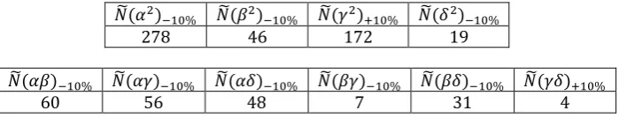
Table-1: Convergence of the Maclaurin series second order coefficients from (35), evaluated as N increases. Set selection intensity 𝜎= 1. Evaluation of formulae (7), (10), (16), (19), (22), (25), (28) and (31), when all multiplied by ½, yield the corresponding coefficients of 𝛼2, 𝛽2, 𝛿2𝛼𝛽, 𝛼𝛾, 𝛼𝛿, 𝛽𝛾 and 𝛽𝛿. The population sizes shown in the Table correspond to a minimum 90% of the asymptotic coefficient values. Note that 𝛼𝛾,𝛼𝛿,𝛽𝛾 and 𝛽𝛿 have negative valued coefficients. Similarly, multiplied by ½, formula (13) of coefficient 𝛾2 and (34) of 𝛾𝛿 converge from above; maximum 110% of their asymptotic values at the population sizes shown.

𝑁�(𝛼2₎

−10% 𝑁�(𝛽2)−10% 𝑁�(𝛾2)+10% 𝑁�(𝛿2)−10%

278 46 172 19

𝑁�(𝛼𝛽)−10% 𝑁�(𝛼𝛾)−10% 𝑁�(𝛼𝛿)−10% 𝑁�(𝛽𝛾)−10% 𝑁�(𝛽𝛿)−10% 𝑁�(𝛾𝛿)+10%

60 56 48 7 31 4

The precision of Table 1 corresponds to absolute errors in small magnitude coefficients and therefore represent conservative convergence thresholds. The selection intensity being a linear scale factor the convergence behaviour of

Table 1 should be robust under varied settings of σ, with the same convergence thresholds.

3. CONCLUSION

Theorem 1 restricts the ‘1/3-rule’ such that selection intensity 𝜛~𝑁−(1+𝑝), where 0≤ 𝑝 ≤1. Such calibrations can be deduced that render the corresponding violations of this evolutionary rule at second order of negligible magnitude. This sharpens the calibration of the selection intensity obtained previously [26]. Quantitative analysis of error thresholds when violation of this rule occurs will clarify this qualitative statement on selection intensity.

Earlier work ([35], equation 19) proposed a dominant quadratic term of the singleton fixation probability series that resembles that obtained from (3) herein, namely [𝑢2(𝑁+ 1)(𝑁+ 2) + 15𝑢𝑣(𝑁+ 1) + 30𝑣2](𝑁−1)(𝑁−2)₃₆₀ , where

𝑢= (𝑎 − 𝑏 − 𝑐+𝑑)/(𝑁 −1) and 𝑣= (𝑁𝑏 − 𝑁𝑑 − 𝑎+𝑑)/(𝑁 −1). This almost yields an asymptotically correct leading order result with inaccuracies that diminish as finite population size N increases, except that it also inflates the result by an order of magnitude in N. Conversely, their lower order terms ([35], equation 19) remain unrecognizable by comparison with those obtained from the precise algebra in parts (i)-(x) of Section 2.1 herein. Their generalization ([35], equation 19) also includes an ill-defined heuristic multiplicative factor [𝑓′(0)]2, where 𝑓(𝛽𝜋) is said to define any function of the product of selection intensity 𝛽 and payoff π (in their notation). Whilst their appendix equation (A.4) does present the correct third order series of the singleton fixation probability that agreed with further calculus, subsequent errors of algebra and a heuristic generalized payoff function incur disagreement.

The work herein suggests a variety of further investigations on mathematical heuristics and alternative statistical processes with which this evolutionary rule arises. These include application of matrix analysis methods [8] and the Kingman coalescent of population genetics [13]. Evolutionary stability concepts in biological games often utilize drift-diffusion partial differential equations [4]. Diffusion theory approaches to the evolutionary rule considered herein have suggested robustness that extends to strong selection [36]. The ‘1/3-rule’ observed in simulation studies where alternative statistical processes model frequency-dependent selection [17] raises further questions about the generality of this evolutionary rule.

REFERENCES

1. Bomze, I., Pawlowitsch, C., One-third rules with equality: second-order evolutionary stability conditions in finite populations, J. Theor. Biol. 254 (2008), 616—620; doi:10.1016/j.jtbi.2008.06.009.

2. Broom, M., Rychtář, J., Game-Theoretical Models in Biology, 1st edn, Chapman and Hall / CRC Press, Boca

Raton, 2013. ISBN 978-1-4398-5321-4.

3. Chalub, F.A.A.C., Souza, M.O., Fixation in large populations: a continuous view of a discrete problem, J. Math. Biol.72 (2016), 283—330; doi: 10.1007/s00285-015-0889-9.

4. Cressman, R., Apaloo, J., Evolutionary game theory, in: Handbook of Dynamic Game Theory, 1st edn (eds T.

Başar and G. Zaccour), Springer Nature, London, 2018. ISBN 978-3-319-44373-7.

5. Fudenberg, D., Nowak, M.A., Taylor, C., Imhof, L.A., Evolutionary game dynamics in finite populations with strong selection and weak mutation, Theor. Popul. Biol.70 (2006), 352—363; doi:10.1016/j.tpb.2006.07.006. 6. Gokhale, C.S., Traulsen, A., Evolutionary multiplayer games, Dyn. Games Appl. 4 (2014), 68—88; doi:

10.1007/s13235-014-0106-2.

7. Graham, R.L., Knuth, D.L. Patashnik, O., Concrete Mathematics: a Foundation for Computer Science, 2nd edn, Addison-Wesley, Upper Saddle River, 1994. ISBN: 978-0-201-55802-9.

8. Imhof, L.A., Nowak, M.A., Evolutionary game dynamics in a Wright-Fisher process, J. Math. Biol. 52 (2006), 667–681; doi: 10.1007/s00285-005-0369-8.

10. Kurokawa, S., Ihara, Y., Emergence of cooperation in public goods games, Proc. R. Soc. B 276 (2009), 1379—1384; doi:10.1098/rspb.2008.1546.

11. Kurokawa, S., Ihara, Y., Evolution of group-wise cooperation: Is direct reciprocity insufficient? J. Theor. Biol. 415 (2017), 20—31; doi:10.1016/j.jtbi.2016.12.002.

12. Kurokawa, S., Generalized version of the one-third law, Research & Reviews: J. Zool. Sci. 5(2) (2017), 52—56; e-ISSN: 2321-6190.

13. Lessard, S., Ladret, S., The probability of fixation of a single mutant in an exchangeable selection model,J. Math. Biol. 54 (2007), 721—744; doi:10.1007/s00285-007-0069-7.

14. Lessard, S., Lahaie, P., Fixation probability with multiple alleles and projected average allelic effect on selection, Theor. Popul. Biol.75 (2009), 266—277; doi:10.1016/j.tpb.2009.01.009.

15. Lessard, S., Evolution of cooperation in finite populations, in: Evolutionary Game Dynamics, Proceedings of Symposia in Applied Mathematics 69 (ed K. Sigmund) (American Mathematical Society, Providence, 2011), 143—156.

16. Lessard, S., On the robustness of the extension of the one-third law of evolution to the multi-player game, Dyn. Games Appl.1 (2011), 408—418; doi: 10.1007/s13235-011-0010-y.

17. Liu, X., He, M., Kang, Y., Pan, Q., Fixation of strategies with the Moran and Fermi processes in evolutionary games, PhysicaA 484 (2017), 336—344; doi:10.1016/j.physa.2017.04.154.

18. Moran, P.A.P., Random processes in genetics, Proc. Camb. Phil. Soc. 54 (1958), 60—71; doi:10.1017/ S0305004100033193.

19. Moran, P.A.P, The effect of selection in a haploid genetic population, Proc. Camb. Phil. Soc. 54 (1958), 463—467; doi:10.1017/S0305004100003017.

20. Moran, P.A.P., Statistical Processes of Evolutionary Theory, 1st edn, Clarendon Press, Oxford, 1962.

21. Nowak, M.A., Sasaki, A., Taylor, C., Fudenberg, D., Emergence of cooperation and evolutionary stability in finite populations, Nature 428 (2004), 646—650; doi: 10.1038/nature02414.

22. Nowak, M.A., Evolutionary Dynamics: Exploring the Equations of Life, 1st edn, Harvard University Press, Cambridge, 2006. ISBN 978-0-674-02338-3.

23. Nowak, M.A., Five rules for the evolution of cooperation, chapter 4 of Part II (Mathematics, Game Theory, and Evolutionary Biology: The Evolutionary Phenomenon of Cooperation), in: Evolution, Games, and God, 1st edn, (eds S. Coakley and M.A. Nowak), (Harvard University Press, Cambridge, 2013), 99—114. ISBN 978-0-674-04797-6.

24. Ohtsuki, H., Bordalo, P., Nowak, M.A., The one-third law of evolutionary dynamics, J. Theor. Biol. 249 (2007), 289—295; doi:10.1016/j.jtbi.2007.07.005.

25. Sample, C., Allen, B., The limits of weak selection and large population size in evolutionary game theory, J. Math. Biol.75 (2017), 1285—1317; doi: 10.1007/s00285-017-1119-4.

26. Slade, P.F., On risk-dominance and the ‘1/3-rule’ in 2 × 2 evolutionary games, Int. J. Pure Applied Math. 113(5) (2017), 649—664; doi:10.12732/ijpam.v113i5.12.

27. Stewart, A.J., Plotkin, J.B., Collapse of cooperation in evolving games, Proc. Natl. Acad. Sci. (U.S.A.) 111(49) (2014), 17558—17563; doi:10.1073/pnas.1408618111.

28. Traulsen, A., Claussen, J.C., Hauert, C., Coevolutionary dynamics: from finite to infinite populations, Phys. Rev. Lett.95 (2005),238701; doi:10.1103/PhysRevLett.95.238701.

29. Traulsen, A., Pacheco, J.M., Imhof, L.A., Stochasticity and evolutionary stability, Phys. Rev. E 74 (2006),

021905; doi:10.1103/PhysRevE.74.021905.

30. Traulsen, A., Shoresh, N., Nowak, M.A., Analytical results for individual and group selection of any intensity, Bull. Math. Biol.70 (2008), 1410—1424; doi: 10.1007/s11538-008-9305-6.

31. Traulsen, A., Hauert, C., Stochastic evolutionary game dynamics, in: Reviews of nonlinear dynamics and complexity 2 (edG. A. Schuster), (Wiley-VCH, Weinheim, 2009), 25—61; doi:10.1002/9783527628001.ch2. 32. Uyenoyama, M., Feldman, M.W., Theories of kin and group selection: a population genetics perspective,

Theor. Popul. Biol.17 (1980), 380—414.

33. Van Cleve, J., Social evolution and genetic interactions in the short and long term, Theor. Popul. Biol.103 (2015), 2—26; doi:10.1016/j.tpb.2015.05.002.

34. Wakeley, J., Coalescent Theory: an Introduction, 1st edn, Roberts and Company Publishers, Greenwood Village, 2009. ISBN 978-0-974-70775-4.

35. Wu, B., Altrock, P.M., Wang, L., Traulsen, A., Universality of weak selection, Phys. Rev. E 82 (2010), 046106; doi:10.1103/PhysRevE.82.046106.

36. Zheng, X.D., Cressman, R., Tao, Y., The diffusion approximation of stochastic evolutionary game dynamics: mean effective fixation time and the significance of the one third law, Dyn. Games Appl.1 (2011), 462—477; doi: 10.1007/s13235-011-0025-4.

Source of support: Nil, Conflict of interest: None Declared.