Task Allocation for Mobile Cloud Computing in Heterogeneous Wireless Networks

(1)

Task Allocation for Mobile Cloud Computing in

Heterogeneous Wireless Networks

Zongqing Lu, Jing Zhao, Yibo Wu and Guohong Cao

Department of Computer Science and Engineering The Pennsylvania State University

E-mail:{zongqing, juz139, yxw185, gcao}@cse.psu.edu

Abstract—The ubiquity of mobile devices creates a rapidly growing market for mobile applications. Many of these applica-tions involve complex processing tasks that are difficult to run on resource constrained mobile devices. This leads to the emergence of mobile cloud computing, in which cloud-based resources are used to enhance the computing capabilities of mobile devices. In this paper, we consider heterogeneous wireless networks in which multiple resource-rich computing nodes can be used as mobile clouds, and mobile devices can upload computation extensive tasks to these mobile clouds. The goal is to minimize the average task response time through determining whether to upload a task, and to which cloud the task should be uploaded. We formalize this task allocation problem, which is proved to be a NP-hard problem, and propose both offline centralized approach and online distributed approach to address this problem. Simulation results show that our approaches outperform others in terms of task response time in various scenarios.

I. INTRODUCTION

The past few years have witnessed an explosive growth of mobile devices (e.g., smartphones, tablets). The ubiquity of mobile devices is accompanied by greater demand for mobile applications such as image processing, speech and optical character recognition, and natural language translation. Many of these applications involve complex processing that requires high computing speed, memory and battery lifetime. However, despite advances in manufacture technology, current mobile devices are still much more resource constrained compared with traditional desktop computers. In many cases, it is hard for these mobile devices to execute these computation exten-sive applications locally.

Recently, the combination of cloud computing and mobile computing leads to a new research area called mobile cloud

computing, in which resource-constrained mobile devices use

cloud-based resources to enhance their computing capabili-ties [1], [2]. For example, Satyanarayana [3] proposes acyber

foraging approach in which mobile devices upload tasks to

some nearby resource-rich computing devices like traditional non-mobile computers. It has been implemented in many systems, such as Spectra [4], Chroma [5] and Scavenger [6]. However, resource-rich computing devices do not always exist in vicinity, which restricts the deployment of such cyber foraging approach. With access to Internet, some other ap-proaches (e.g., MAUI [7] and CloneCloud [8]) upload tasks to the remote cloud infrastructure. In scenarios without Internet access, a group of mobile devices (connected by WiFi or Bluetooth) can form a mobile cloud to cooperatively run their tasks [9], [10], [11]. However, these works do not consider and

exploit the heterogeneity of these mobile nodes in the network; i.e., some mobile nodes have low computation power whereas other mobile nodes have much higher computation power.

In this paper, we consider heterogeneous wireless networks in which multiple resource-rich computing nodes can be used as mobile clouds, and mobile devices can upload computation extensive tasks to these mobile clouds. For example, in bat-tlefields, mobile clouds can be mobile nodes like computers inside tanks that have much higher computation power than mobile devices carried by solders, or they can be powerful computation devices at command center or other moving vehicles. The goal is to minimize the average task response time through determining whether to upload a task, and to which mobile cloud the task should be uploaded. The task response time may be affected by several factors such as processing delay, communication delay and queuing delay at mobile clouds. Always uploading tasks to the nearest mobile cloud may reduce the communication delay, but its queuing delay may be long if that mobile cloud has to process many requests. Thus, we have to carefully consider all three factors to minimize the task response time.

We first formalize the task allocation problem in heteroge-neous wireless network, and prove that it is NP-hard. Based on the technique of linear programming relaxation [12], we propose an offline centralized approach to solve it. Then, we propose an online distributed approach in which the information of future tasks are not known in advance. The basic idea is for each mobile node to collect some network information and make task allocation decisions by themselves. Through extensive simulations, we investigate the tradeoff between performance and overhead, and demonstrate that our approaches can significantly outperform other approaches in terms of task response time.

The remainder of the paper is organized as follows. Sec-tion II provides an overview of our approaches and the problem formulation. Section III and Section IV describe the offline centralized algorithm and the online distributed algorithm, respectively. Evaluation results are presented in Section V and Section VI concludes the paper.

II. OVERVIEW A. The Big Picture

We consider a heterogeneous wireless network formed by mobile clouds and mobile devices based on ad hoc connec-tions. Since mobile devices usually have limited moving speed

(2)

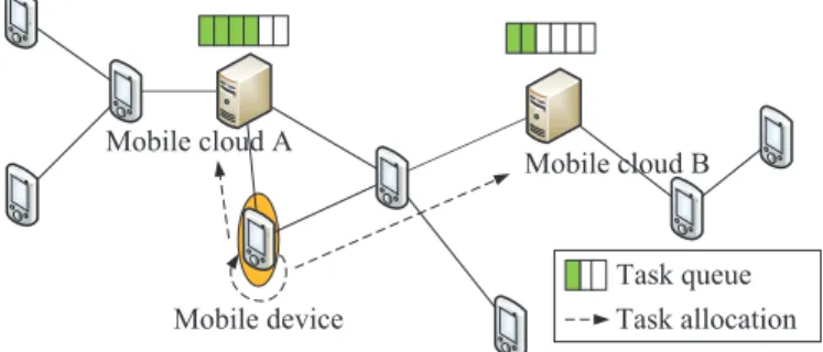
(e.g., they are carried by soldiers in battlefields), we assume their relative position to mobile clouds may not change too much during a short period of time, so the network can be modeled as a graph shown in Figure 1. Each mobile device generates a number of tasks over time and may upload them to some mobile clouds. It is possible that a mobile cloud is busy processing some existing tasks and has to put the new task into a waiting queue. In our model, each mobile cloud maintains a queue to buffer pending tasks which cannot be immediately processed. Tasks in the queue are processed on a first-come-first-serve basis, and the queuing delay may differ from one mobile cloud to another.

As shown in Figure 1, suppose a new task is generated by the mobile device encircled. The task can be completed by itself or uploaded to mobile cloud A or B. To upload the task, the task response time may be affected by several factors such as the processing delay at the mobile cloud, the communication delay from the mobile device to the mobile cloud, and the queuing delay at the mobile cloud. In this example, allocating the task to mobile cloud A incurs less communication delay than mobile cloud B, since there are fewer hops between mobile cloud A and the task generator. However, as mobile cloud A has more neighboring nodes (than mobile cloud B), mobile cloud A generally has higher task queuing delay. Thus, these three factors should be jointly considered to find the optimal task allocation.

In this paper, we address the task allocation problem under two settings: centralized setting and distributed setting.

1) Centralized Setting: Suppose all task information is

known as a priori. Then, the task allocation problem can be reduced to the NP-hard scheduling problem [13] which schedules a number of jobs (tasks) on multiple nodes. We can design a centralized scheme based on the technique of linear programming relaxation [12]. Specifically, the problem can be formulated as an integer linear programming problem, and then the integer constraint (each variable must be 0 or 1) can be replaced by a weaker constraint (each variable belongs to [0,1]). The resulting relaxation is a linear program, which can be solved by GLPK [14] in polynomial time. Finally, we transform the solution to meet the integer constraint, and then derive the task allocation decisions.

2) Distributed Setting: In practice, the information of future

tasks is not known as a priori, and we propose a distributed ap-proach in which each mobile device makes allocation decisions locally. More specifically, when a new task is generated, the task generator makes a greedy allocation decision to minimize the response time of that task. To achieve this, the task generator has to collect the information about processing delay, communication delay and queuing delay of mobile clouds. Here the queuing delay of a mobile cloud is frequently updated whenever a new task is received, so each mobile cloud has to periodically broadcast its queuing delay to inform all task generators (mobile devices). By increasing the frequency of broadcast, the information collected by the task generator will be more accurate. Then, the task generator will most likely make good allocation decisions, but at the cost of more control

Task queue Mobile cloud B Mobile cloud A

Mobile device Task allocation

Fig. 1: Network Scenario

message overhead. The tradeoff between performance and overhead will be investigated in the performance evaluation section.

B. Problem Formulation

We first describe the network model and the task model, and then formulate the task allocation problem.

1) Network Model: The network is modeled as a graph

G(V, E), where each node i ∈ V corresponds to either a mobile cloud or a mobile device, and an edge e ∈ E

represents the link between the two end nodes if they fall in the communication range. Each edge is associated with the communication link delay. In general, for any two nodes i1

and i2, the communication delay between them is modeled by the length of the shortest i1-i2 path in Gwhere the edge

weight is the communication link delay. Note that it can be obtained by Dijkstra’s shortest path algorithm [15].

2) Task Model: There are a number of tasks generated in

the network. Let pi,j be the processing delay of task j if it is processed by nodei. A task can be processed by either its generator or a mobile cloud who has much shorter processing delay than the generator, and the processing delay by any other node (except the generator or mobile cloud) is infinity long. LetTi,j be the time if taskj is completed by nodei, then

Ti,j=tj+ 2di,j+qi+pi,j

wheretj is the generation time of taskj,di,jis the communi-cation delay between nodeiand the generator of task j, and

qi is the queuing delay at nodei.

LetTj be the complete time of task j. Then,

Tj = min i∈V Ti,j and the response time of task j isTj−tj.

We formulate the task allocation problem as follows.

Definition 1: Task Allocation Problem

Given a set of tasks (denoted byU) to be completed by nodes in a heterogeneous wireless network, how to allocation tasks to minimize the average task response time _|_U1_|_j_∈_U(Tj−tj)? Note that _|_U1_|_j_∈_U(Tj−tj) = _|_U1_|j∈UTj−_|_U1_|j∈Utj and _|_U1_|_j_∈_Utj is a constant, so we simplify the objective to minimize the average task complete time _|_U1_|_j_∈_UTj.

(3)

III. OFFLINECENTRALIZEDAPPROACH

In this section, we first reduce the task allocation problem to the scheduling problem for proving the NP-hardness, and then propose a centralized algorithm based on linear programming relaxation.

A. Reduction to the Scheduling Problem

Definition 2: Scheduling Problem

Given a set of jobs (denoted by U) to be completed by a number of nodes. Each job j is associated with a positive weight wj, a nonnegative processing time and a nonnegative release time (i.e., the earliest possible start time) on each node. The jobs must be processed without interruption, and a node can process at most one job at a time. Let Tj denote the complete time of job j, how to schedule jobs to minimize the average job complete time _|_U1_|_j_∈_UwjTj?

Theorem 1: The scheduling problem is NP-hard [13].

The task allocation problem can be reduced to the schedul-ing problem as follows: each task corresponds to a job, and the task arrival time corresponds to the job release time. Our goal is to minimize the average task complete time, which corresponds to minimizing the weighted job complete time in the scheduling problem by assigning unit weight to every task. Since the scheduling problem is NP-hard, we have the following theorem.

Theorem 2: The task allocation problem is NP-hard.

B. Algorithm Description

1) Linear Programming Relaxation: Letndenote the

num-ber of nodes andmdenote the number of tasks. We formulate our problem as the following integer linear programming problem. minimize 1 m n i=1 m j=1 h k=1 τk−1xi,j,k (1) subject to n i=1 h k=1 xi,j,k= 1 (2) m j=1 h k=1 pi,jxi,j,k≤τk, h= 1,2, . . . , h (3)

xi,j,k= 0 ifτk< tj+di,j+pi,j (4)

xi,j,k∈ {0,1} (5)

Here we divide the time horizon into the following intervals:

[1,1],(1,2],(2,4],. . .,(2h−2,2h−1], wherehis the smallest integer such that

2h−1_≥_max i,j (tj+di,j) + m j=1 max

i,pi,j<∞pi,j

That is, 2h−1 is the latest possible time when all tasks are completed. For conciseness, let τ0 = 1, τk = 2k−1 (k =

1,2, . . . , h), so thekth interval can be denoted by (τk−1, τk] (k= 1,2, . . . , h).

In the program,xi,j,kindicates whether taskj is scheduled to complete on nodeiwithin the interval (τk−1, τk]. Ifxi,j,k is 1,τk−1 is used as an approximation of the actual complete

time to calculate the average task complete time (the objective function (1)). Constraint (2) ensures that only one node is scheduled to complete each task. Constraint (3) ensures that the complete time requirement indicated byxi,j,k is satisfied. Constraint (4) ensures that each taskj that completes by time

τk on node imust havetj+di,j+pi,j≤τk.

Since the program has an integer constraint (Constraint (5)), there is no polynomial time algorithm to find the so-lution. Thus, we relax Constraint (5) to Constraint (6) and use GLPK [14] to solve the linear program (1)-(4),(6) in polynomial time.

xi,j,k≥0 (6)

2) Rounding: Let x∗_i,j,k denote the solution for the linear

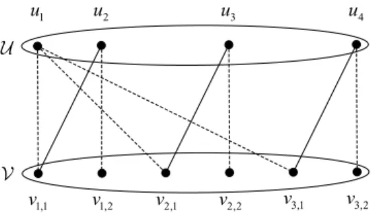
program (1)-(4),(6). However, x∗_i,j,k may be fractional, and hence does not represent a feasible solution to the task allocation problem. We apply the rounding technique [16] to transform x∗i,j,k into integers by constructing a weighted bipartite graphG(U,V,E). One side of the bipartite graph has the tasks, i.e.,

U ={uj|j= 1,2, . . . , m} The other side has the nodes, i.e.,

V ={vi,s|i= 1,2, . . . , n;s= 1,2, . . . , si} where si = mj=1

_h

k=1xi,j,k, and the si vertices {vi,s|s= 1,2, . . . , si}correspond to nodei.

For conciseness, letxi,j denoteh_k₌₁xi,j,k. The edges of the bipartite graph correspond to node-task pairs (i, j) such thatxi,j>0. More specifically, the edges connecting vertices {vi,s|s= 1,2, . . . , si}are constructed as follows:

1) Find the smallest indexj1 such thatji=11 xi,j≥1. 2) For j = 1,2, . . . , j1 −1, if xi,j > 0, add an edge

(uj, vi,1)with weight xi,j.

3) Add an edge(uj1, vi,1)with weight1−

_j₁₋₁

i=1 xi,j. This

ensures that the total weight of edges connectingvi,1 is at most 1.

4) Ifj_i₌₁1 xi,j > 1, add an edge (uj1, vi,2) with weight

j1

i=1xi,j−1.

5) In a similar way, continue adding edges to

vi,2, vi,3, . . . , vi,si.

Based on the matching theory [17], there exists a matching in bipartite graphG(U,V,E)which matches all tasks inU. We use the Hungarian algorithm [18] to find a maximum weighted matching whose total edge weight is the maximum among all matchings. If an edge(uj, vi,s)is in the matching, we setx¯i,j to 1; otherwise,x¯i,j is set to 0. This minimizes the difference between the fractional solution xi,j and the rounding result

¯ xi,j.

(4)

. -1 u u2 u3 u4 1,1 v v1,2 v2,1 v2,2 v3,1 v3,2

Fig. 2: An example bipartite graph. The weight of solid edge is 2/3, and the weight of dashed edge is 1/3.

Algorithm 1 Offline Centralized Algorithm

Input: task setU, node setV, andtj,di,j,pi,jfor∀i∈V, j∈ U

1: Calculate handτ_k,k= 0,1, . . . , h 2: Solve linear program (1)-(4),(6) by GLPK

3: Construct weighted bipartite graph G based on the frac-tional solution xi,j,k

4: Run Hungarian algorithm to find a maximum weighted bipartite matchingx¯i,j

5: Output the task allocation decisions

We use an example to illustrate the aforementioned proce-dure. Suppose we are given the following(xi,j).

(xi,j) = ⎡ ⎣1₁/_/3 1 0 0_{3 0 1 0} 1/3 0 0 1 ⎤ ⎦

The corresponding bipartite graph is shown in Figure 2. The maximum weighted matching is (u1, v1,1), (u2, v1,2),

(u3, v2,1), (u4, v3,1), which corresponds to the following

(¯xi,j). (¯xi,j) = ⎡ ⎣1 1 0 0_{0 0 1 0} 0 0 0 1 ⎤ ⎦

3) Deriving the Task Allocation Decisions: A task j is

allocated to node i if x¯i,j > 0. If there are multiple tasks allocated to node i, they are scheduled in a non-descending order of the task arrival time.

The entire flow of offline centralized algorithm is summa-rized in Algorithm 1.

IV. ONLINEDISTRIBUTEDAPPROACH

In this section, we first describe how to collect the required information, and then propose a distributed algorithm.

A. Information Collection

Suppose a new task j is generated by node i0. Node i0

makes the task allocation decision based on the following information of each candidate node i(i.e., either nodei0 or a

mobile cloud):

• Communication delay (di,j): As aforementioned in

Sec-tion II-B1, di,j can be obtained by running Dijkstra’s

Protocol 1Information Dissemination Protocol For each mobile cloud:

1: if node profile is updatedthen

2: Broadcast message (node id,profile,timestamp) to all neighboring nodes

3: end if

4: if timestamp−last timestamp≥T then

5: Ifqueuing delay=last queuing delay, broadcast

mes-sage(node id,queuing delay,timestamp) to all

neigh-boring nodes

6: last queuing delay←queuing delay

7: last timestamp←timestamp

8: end if

For each mobile device:

1: if message (node id,profile,timestamp) is received and

timestamp is newer then

2: Broadcast the message to all neighboring nodes and update(node id,profile,timestamp)in record

3: end if

4: if message (node id,queuing delay,timestamp) is re-ceived and timestampis newer then

5: Broadcast the message to all neighboring nodes and update(node id,queuing delay,timestamp)in record

6: end if

shortest path algorithm on graphG. However, such cen-tralized algorithm is difficult to implement in a distributed environment where nodei0do not have the entire network

information. This issue is addressed as follows. Similar to routing discovery in AODV [19], node i0 discovers

a number of paths to node i, during which the delay information of each path is also collected. Node i0

records the path with the minimum delay, whose value is assigned to di,j.

• Queuing delay (qi):As aforementioned in Section II-A,

qi is frequently updated whenever a new task arrives at nodei. Thus, nodei0has to be informed of the up-to-date

qi periodically. This will be achieved by the following information dissemination protocol.

• Processing delay (pi,j):As in several prior work [7], [8],

[9], pi,j can be obtained based on the node profile of node i and the execution profile of task j. Here a node profile includes the execution speed which is estimated by running benchmarks [20]; an execution profile includes the CPU cycles required for running the task. A node profile remains relatively stable over a long period of time. In case of an update, the node will share with all other nodes by the following information dissemination protocol.

The formal description of the information dissemination protocol is shown in Protocol 1, which consists of two parts: at mobile cloud side and at mobile device side.

• At mobile cloud side: Whenever the node profile is

updated, the mobile cloud broadcasts the up-to-date node profile through message (node id,profile,timestamp).

(5)

Algorithm 2 Online Distributed Algorithm at Nodei0

Input: task j and the collected information

1: _V₀← {_i₀}the set of mobile clouds

2: foreach nodeiinV0 do

3: _T_i,j←_t_j+ 2_d_i,j+_q_i+_p_i,j

4: end for

5: _i₁←the node whoseTi,j is the smallest among the nodes inV0

6: Send taskj to nodei1 along the predetermined shortest

i0-i1 path

Here node id denotes the ID which is unique to each

node, and timestampdenotes the time when sending the message. Each mobile cloud also checks whether the queuing delay is different from the last recorded value everyT time units. If there is an update, the mobile cloud broadcasts the up-to-date queuing delay to all neighboring nodes. The effect of T on network performance in will be investigated in Section V.

• At mobile device side: When receiving a message about

node profile (or queuing delay), the mobile device checks whether the timestamp of the message is newer compared with the recorded information. If so, it updates the recorded information and re-broadcasts the message, in order to inform all other mobile devices about the update.

B. Algorithm Description

When a new task is generated, the task generator tries to make a greedy allocation decision to minimize the complete time of that task. More specifically, it uses the collected information to estimate the complete time for each possible task allocation. Then, the task is sent to the node with the minimum complete time. Here the generator includes in the task the predetermined shortest path (as aforementioned in Section IV-A) as a subfield, so other nodes in the network know to which node to forward the task. Through this source routing approach, the communication delay is minimized and thus the quality of task allocation is ensured. The online distributed algorithm is summarized in Algorithm 2.

V. PERFORMANCEEVALUATIONS

In this section, we evaluate the performance of the designed solutions through extensive simulations, which includes two parts: the first part compares the offline and online approaches, and the second part compares the online approach with other approaches based on the NS-3 network simulator.

A. Comparison between Offline and Online Approaches

1) Simulation Setup: To obtain the future task information

required for the offline approach, we set up a simple simulation scenario and then compare it with the online approach. In our simulations, we randomly place 50 mobile devices and 5 mobile clouds in a 3000m × 3000m square area. The transmission range is 250m. If two nodes are within the transmission range, there is a link between them. The default wireless bandwidth is set to 24Mbps. As in previous study [9],

2 4 6 8 10 12 14 16 18 20 0 2 4 6 8 10 12 14

information dissmination period (s)

average task response time (s)

Online

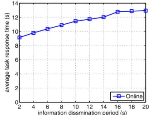
Fig. 3: Effect of information dissemination period

large tasks can be divided into multiple uniform small tasks. The task size, i.e., the size of code and data, is set to 2Mb. For each task, the processing delay by a mobile device is 20s, while the processing delay by a mobile cloud is 2s. Here we do not investigate the scenarios that different mobile clouds have different computing speed, which will be left as future work. The tasks are generated in a homogeneous Poisson process. Due to the memoryless property of Poisson process, the task generation interval follows an exponential distribution.

2) Tradeoff in Information Dissemination: Figure 3 shows

the effect of information dissemination period T on the average task response time. Here the mean task generation interval is set to 18s. The average response time increases as

T increases. AsT increases, the accuracy of the information collected by the task generators decreases. Then, these nodes are less likely to make good allocation decisions, which leads to the increase of average response time. When T increases from 2s to 10s, the average response time increases by 25%. When T further increases from 10s to 20s, the average response time only increases by 13%.

3) Performance Comparisons: Figure 4 shows the

perfor-mance of offline and online approaches in various settings. Since the computational complexity of the offline approach increases significantly as the number of tasks increases, the offline approach is evaluated using a trace of 500 tasks. The offline approach is compared with the online approach under different settings of information dissemination periodT. Note that the mean task generation interval is set to 30s in default. Figure 4a shows the effect of task generation interval on the average task response time. As shown in the figure, with the increase of task generation interval, the average task response time decreases for both offline and online approaches, because longer task generation interval results less queuing delay at mobile clouds. In addition, the online approach with smaller information dissemination period T has better performance. Figure 4b shows the effect of the number of mobile clouds on the average task response time. As expected, the increase of mobile clouds reduces the number of tasks processed at each mobile cloud, and thus decreases the average task response time. When the number of mobile clouds further increases, there is no queuing delay at mobile clouds and thus the task response time that only includes processing delay and communication delay becomes stable. Figure 4c shows the

(6)

10 14 18 22 26 30 0 5 10 15 20 25 30

mean task generation intervel (s)

Offline Online(T=6s) Online(T=12s) Online(T=18s)

(a) effect of mean task generation interval

1 2 3 4 5 6 0 5 10 15 20 25 30 # of mobile clouds

(b) effect of # mobile clouds

2 4 6 8 10 0 5 10 15 20 25 30

processing speed ratio

(c) effect of processing speed ratio Fig. 4: Performance of offline and online approaches when 500 tasks are generated in various settings, where the default processing delay at mobile devices is 20s, the default processing delay at mobile clouds is 2s, the default number of mobile clouds is 5, and the default value of mean task generation interval is 30s.

effect of processing speed ratio on the average task response time. Here we fix the processing delay by a mobile device to 20s, and denote the processing speed ratio as the ratio between the processing time by a mobile device and that by a mobile cloud. Similarly, the average task response time decreases when the processing speed ratio increases, because smaller processing delay leads to less queuing delay at mobile clouds.

As illustrated in Figure 4, the offline approach outperforms the online approaches; among the online approaches, smaller information dissemination period corresponds to better perfor-mance.

B. Comparisons between Online Approach and Other Ap-proaches

1) Simulation Setup: To simulate more realistic network

environments, we use NS-3 simulator to more accurately capture the characteristics of heterogeneous wireless networks. The simulation setup is similar as before. We randomly place 50 mobile devices and 5 mobile clouds in 3000m × 3000m area. Nodes move according to the random waypoint mobility model with a speed randomly chosen between 2 and 5m/s for mobile devices and between 5 and 10m/s for mobile clouds, and there is no pause time. WiFi ad hoc mode is used for wireless communication with a rate 24Mb/s rate (802.11a) and a Friis loss model. The transmission power is set to 17 dBm. The information dissemination protocol is implemented with broadcast interval 6 seconds to collect the information required for the online approach. Tasks are generated in Poisson processes and the mean task generation interval for each mobile device is randomly chosen between 40s and 60s or between 60s and 120s or between 120s and 180s. The task size is set to 1Mb or 2Mb. Tasks are transmitted through TCP connections. The processing delay at mobile clouds is set to 10s, and the processing delay at mobile devices is set to 50s or 100s. Each simulation runs for one hour.

We compare our online approach with the following ap-proaches:

• Random: The task generator randomly selects a mobile

cloud to allocate the task.

• Nearest:The task generator selects the mobile cloud with

the minimum communication delay for task allocation.

• Local:All tasks are completed by the task generator itself

(i.e., not uploaded to any mobile cloud).

2) Performance Comparisons: Figure 5 shows the

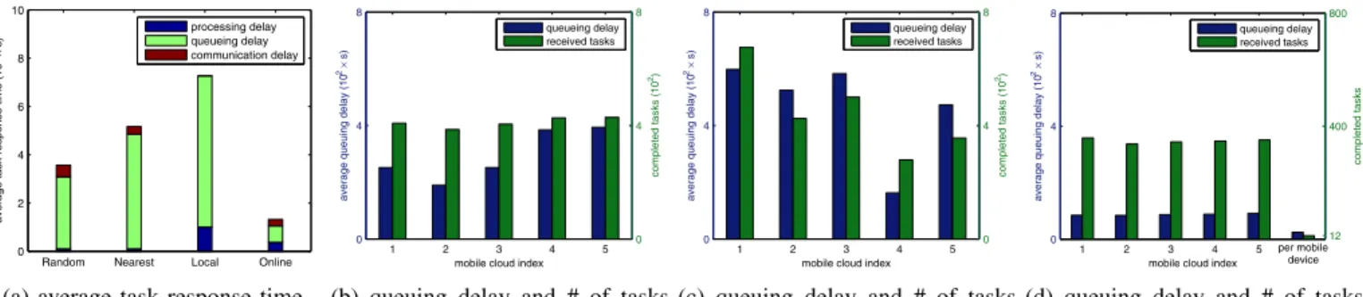
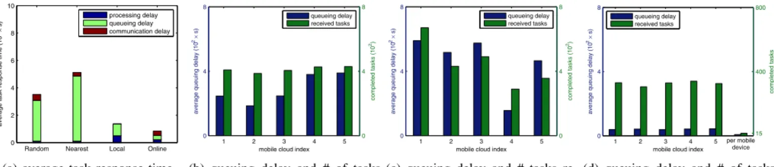
perfor-mance of these approaches when the processing delay at mobile devices and mobile clouds is 100s and 10s, respec-tively, and the mean task generation interval is randomly chosen between 60s and 120s for each mobile device. Figure 5a compares the four approaches in terms of average task response time which consists of processing delay, queueing delay, and communication delay. Among them, Online per-forms the best and the task response time is much less than the other three approaches, while Local performs the worst. For all these approaches, the proportion of the queuing delay in the task response time is large, but the queuing delay of

Online is much less than other approaches. Random has the

highest communication delay, becauseRandomallocates tasks to a randomly selected mobile cloud without considering the communication delay and hence the communication delay of the task can be very long when the task generators is far from the selected mobile cloud. SinceOnlineprocesses some tasks locally (no communication delay), it has less communication delay than N earest on average and the processing delay is also between 10s and 100s. Local does not incur any communication delay since it only processes tasks locally.

Onlineoutperforms others in terms of average task response

time because it considers the processing delay, communication delay and queue delay jointly while the other three approaches could not.

Figures 5b, 5c and 5d show the average queuing delay and the number of received tasks at each mobile cloud (also locally processed tasks for Online) for Random,Nearest and

Online, respectively. From these figures, we can seeRandom

allocates tasks more equally thanNearestandOnline.Nearest

(7)

Random Nearest Local Online 0 2 4 6 8 10

average task response time (10

2×

s)

processing delay queueing delay communication delay

(a) average task response time

1 2 3 4 5

0 4 8

mobile cloud index

average queuing delay (10

2× s) 0 4 8 completed tasks (10 2) queueing delay received tasks

(b) queuing delay and # of tasks received at each mobile cloud for

Random

1 2 3 4 5

0 4 8

mobile cloud index

(c) queuing delay and # of tasks received at each mobile cloud for

Nearest

1 2 3 4 5

0 4 8

mobile cloud index

2× s) per mobile device 12 400 800 completed tasks queueing delay received tasks

(d) queuing delay and # of tasks received at each mobile cloud for

Online

Fig. 5: Performance ofRandom,Nearest,LocalandOnlinewhen the task size is 1Mb, the processing delay at mobile devices and mobile clouds is 100s and 10s, respectively, and the mean task generation interval is between 60s and 120s.

Random Nearest Local Online 0

1 2 3

2×

s)

1 2 3 4 5

0 1 2

mobile cloud index

Random

1 2 3 4 5

0 1 2

mobile cloud index

Nearest

1 2 3 4 5

0 1 2

mobile cloud index

2× s) per mobile device 1 200 400 com p leted tasks queueing delay received tasks

Online

communication delay and thus tasks can gather at some specific mobile cloud if there are many mobile devices nearby, e.g., mobile cloud 1 in Figure 5c.Onlineallocates tasks evenly on each mobile cloud (about 350 tasks at each mobile cloud) and allocates 12 tasks at each mobile device on average, as shown in Figure 5d. Moreover, the average queuing delay at mobile devices is much less than that at mobile clouds (i.e., about 20 seconds at mobile devices and 80 seconds at mobile clouds.

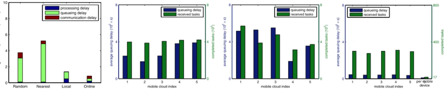
Figure 6 shows the performance of these approaches when tasks are generated at each mobile devices with the mean interval between 120s and 180s. Since less tasks are generated compared to Figure 5, the queueing delay at mobile clouds and mobile devices decreases and thus the average task response time of all these approaches drops significantly as shown in Figure 6a, whereOnlinestill outperforms others. ForRandom

andNearest, as shown in Figures 6b and 6c, the distribution of

tasks at each mobile cloud is similar as in Figures 5b and 5c, however the number of tasks and the queuing delay at each mobile cloud decrease. For Online, as shown Figure 7d due to the reduction of queuing delay at mobile clouds, Online

are more likely to allocate tasks at mobile cloud and very few tasks are allocated at mobile devices (less than 1 task per mobile device).

Figure 7 shows the performance of these approaches when

the processing delay at mobile devices is set to 50s and the mean task generation interval is between 60s and 120s. As shown in Figure 7a, the task response time of Local

decreases significantly due to the reduced processing delay at mobile devices, compared to Figure 5a. Since the change of processing delay at mobile devices does not affect the task allocation decisions ofRandomandNearest, their performance is similar as in Figure 5. ForOnline, the average task response time also decreases due to the reduced processing delay and queuing delay. As shown in Figure 7d, Online allocates less tasks at mobile clouds and more tasks at mobile devices compared to Figure 5d. Due to the reduced processing delay at mobile devices, processing tasks locally is more likely to obtain better task response time when the queuing delay at mobile clouds is high.

In Figure 8, we set the mean generation interval between 40s and 60s and keep other parameters same as in Figure 7. As shown in Figure 8a, the average task response time of all these approaches increases, compared to Figure 7a, due to the increased queuing delay incurred by more generated tasks. For RandomandNearest, although the generated tasks increase, the distribution of tasks among mobile clouds is similar with Figures 7b and 7c, respectively. When more tasks are generated, Online tends to process more tasks locally due to the increased queuing delay at mobile clouds and

(8)

2×

s)

1 2 3 4 5

0 4 8

mobile cloud index

Random

1 2 3 4 5

0 4 8

mobile cloud index

(c) queuing delay and # tasks re-ceived at each mobile cloud for

Nearest

1 2 3 4 5

0 4 8

mobile cloud index

Online

2×

s)

1 2 3 4 5

0 6 12

mobile cloud index

Random

1 2 3 4 5

0 6 12

mobile cloud index

Nearest

1 2 3 4 5

0 6 12

mobile cloud index

Online

the raised communication delay (incurred by the increased network traffic); i.e., 37 tasks on average are allocated at each mobile device in Figure 8d, while 15 tasks are processed locally at each mobile device in Figure 7d.

Finally, we investigate how the task size affects the perfor-mance of these approaches. Figure 9 shows the results when the task size is set to 2Mb, the processing delay at mobile devices is set to 50s, and the mean task generation interval is between 60s and 120s. Compared to Figure 7a where the task size is 1Mb, the communication delay ofRandomandNearest

increases due to the increase of task size, and thus the average task response time also increases, as shown in Figure 9a. Since the task size does not affect Local, its performance is the same as in Figure 7a. For Online, due to the increase of communication delay to mobile clouds,Onlineallocates more tasks at mobile devices and less tasks at mobile clouds than that in Figure 7d. Moreover, tasks are balanced among mobile clouds as before.

Figure 10 shows the results when the task size is 2Mb and the tasks are generated more frequently (the mean task generation interval is between 40s and 60s). As shown in Figure 10a, due to the increase of task size, the communication delay of Random, Nearest and Online increases, compared to Figure 8a. Moreover, comparing to Figure 9a, since more tasks are generated, the queueing delay increases for all

these approaches. Due to the increase of task size, Online

is more likely to allocate tasks at mobile devices, when the communication delay to mobile clouds is high, so as to achieve better task response time.

In summary, Random allocates tasks randomly at mobile clouds;Nearestallocates more tasks at the mobile clouds that have more mobile devices in vicinity;Local always allocates tasks locally at mobile devices;Onlineallocates tasks at mo-bile clouds and momo-bile device accordingly to minimize the task response time, considering the queuing delay, communication delay and processing delay together. Therefore,Onlineadapts to the variations of parameter settings and outperforms other approaches in all simulation settings.

VI. CONCLUSIONS

This paper studied the task allocation problem for mobile cloud computing in heterogeneous wireless networks, where multiple resource-rich computing nodes can be used as mobile clouds, and mobile devices can upload computation extensive tasks to these mobile clouds. The objective is to minimize the average task response time of all tasks considering communi-cation delay, queuing delay and processing delay. To address this NP-hard problem, we first designed an offline central-ized approach based on the technique of linear programming relaxation and then proposed an online distributed approach.

(9)

2×

s)

1 2 3 4 5

0 4 8

mobile cloud index

Random

1 2 3 4 5

0 4 8

mobile cloud index

Nearest

1 2 3 4 5 0

0 4 8

mobile cloud index

Online

2×

s)

1 2 3 4 5

0 6 12

mobile cloud index

Random

1 2 3 4 5

0 6 12

mobile cloud index

Nearest

1 2 3 4 5

0 6 12

mobile cloud index

Online

Evaluation results show that our approaches outperform others in terms of task response time in various scenarios.

REFERENCES

[1] H. T. Dinh, C. Lee, D. Niyato, and P. Wang, “A survey of mobile

cloud computing: architecture, applications, and approaches,”Wireless

Communications and Mobile Computing, vol. 13, no. 18, pp. 1587–1611, 2013.

[2] Z. Sanaei, S. Abolfazli, A. Gani, and R. Buyya, “Heterogeneity in

Mobile Cloud Computing: Taxonomy and Open Challenges,” IEEE

Communications Surveys & Tutorials, vol. 16, no. 1, pp. 369–392, 2014.

[3] M. Satyanarayanan, “Pervasive computing: vision and challenges,”IEEE

Personal Communications, vol. 8, no. 4, pp. 10–17, 2001.

[4] J. Flinn, S. Park, and M. Satyanarayanan, “Balancing performance,

energy, and quality in pervasive computing,” inProceedings of IEEE

International Conference on Distributed Computing Systems, 2002. [5] R. K. Balan, D. Gergle, M. Satyanarayanan, and J. Herbsleb,

“Sim-plifying cyber foraging for mobile devices,” inProceedings of ACM

International Conference on Mobile Systems, Applications, and Services, 2007.

[6] M. D. Kristensen, “Scavenger: Transparent development of efficient

cyber foraging applications,” in Proceedings of IEEE International

Conference on Computer Communications, 2010.

[7] E. Cuervo, A. Balasubramanian, D. Cho, A. Wolman, S. Saroiu, R. Chandra, and P. Bahl, “MAUI: making smartphones last longer

with code offload,” inProceedings of ACM International Conference

on Mobile Systems, Applications, and Services, 2010.

[8] B. Chun, S. Ihm, P. Maniatis, M. Naik, and A. Patti, “CloneCloud:

Elastic execution between mobile device and cloud,” inProceedings of

ACM European Conference on Computer Systems, 2011.

[9] C. Shi, V. Lakafosis, M. H. Ammar, and E. W. Zegura, “Serendipity: Enabling Remote Computing among Intermittently Connected Mobile

Devices,” inProceedings of ACM International Symposium on Mobile

Ad Hoc Networking and Computing, 2012.

[10] Y. Li and W. Wang, “Can Mobile Cloudlets Support Mobile

Applica-tions,” inProceedings of IEEE International Conference on Computer

Communications, 2014.

[11] A. Fahim, A. Mtibaa, and K. A. Harras, “Making the case for

com-putational offloading in mobile device clouds,” inProceedings of ACM

International Conference on Mobile Computing and Networking, 2013. [12] L. A.Hall, A. S. Schulz, D. B. Shmoys, and J.Wein, “Scheduling to minimize average completion time: Off-line and on-line approximation

algorithms,”Mathematics of Operations Research, vol. 22, no. 3, pp.

513–544, 1997.

[13] J. K. Lenstra, A. H. G. R. Kan, and P. Brucker, “Complexity of machine

scheduling problems,”Annals of Discrete Mathematics, vol. 1, pp. 343–

362, 1977.

[14] GLPK: GNU Linear Programming Kit, “http://www.gnu.org/software/ glpk/glpk.html.”

[15] E. W. Dijkstra, “A note on two problems in connexion with graphs,” Numerische Mathematik, vol. 1, no. 1, pp. 269–271, 1959.

[16] D. B. Shmoys and E. Tardos, “An approximation algorithm for the

generalized assignment problem,”Mathematical Programming, vol. 62,

no. 1-3, pp. 461–474, 1993.

[17] L. Lovasz and M. D. Plummer,Matching Theory. American

Mathe-matical Society, 2009.