ISSN: 1311-1728 (printed version); ISSN: 1314-8060 (on-line version)
doi:http://dx.doi.org/10.12732/ijam.v31i4.4
CONSTRUCTION OF COMPLEX NESTED IDEAL LATTICES FOR COMPLEX-VALUED
CHANNEL QUANTIZATION C. C. Trinca Watanabe 1§, J.-C. Belfiore 2,
E. D. De Carvalho 3, J. Vieira Filho4, R. Palazzo Jr. 1, R. A. Watanabe 5 1 Department of Communications (DECOM)
Campinas State University Campinas-SP, 13083-852, BRAZIL
2 Department of Communications and Electronics T´el´ecom ParisTech
Paris, 75013, FRANCE 3 Department of Mathematics
S˜ao Paulo State University Ilha Solteira-SP, 15385-000, BRAZIL
4 Telecommunications Engineering S˜ao Paulo State University
S˜ao Jo˜ao da Boa Vista-SP, 13876-750, BRAZIL 5 Institute of Mathematics, Statistics and
Scientific Computation (IMECC) Campinas State University Campinas-SP, 13083-852, BRAZIL
Abstract: In this work we develop a new algebraic methodology which quan-tizes complex-valued channels in order to realize interference alignment (IA) onto a complex ideal lattice. Also we make use of the minimum mean square error (MMSE) criterion to estimate complex-valued channels contaminated by additive Gaussian noise.
Received: March 14, 2018 c 2018 Academic Publications
AMS Subject Classification: 03G10, 06B05, 06B10, 11RXX, 13F10, 97N20 Key Words: complex ideal lattices; nested lattices; binary cyclotomic field; principal ideal rings; channel quantization
1. Introduction
In this work we make use of rotated complex lattices constructed through exten-sion fields to develop a new algebraic methodology to perform a complex-valued channel quantization in order to realize interference alignment (IA) [1] onto a complex ideal lattice.
In a wireless network a transmission from a single node is heard not only by the intended receiver, but also by all other nearby nodes. Each node, indexed by m = 1,2, . . . , M, observes a noisy linear combination of the transmitted signals through the channel
ym= L
X
l=1
hmlxl+zm, (1.1)
where hml ∈ C are complex-valued channel coefficients, xl is a complex
lat-tice point whose message space presents a uniform distribution and zm is an
i.i.d. circularly symmetric complex Gaussian noise. Figure 1 illustrates the corresponding channel model.
Figure 1: A Gaussian Multiple-Access Channel
partitioning of that lattice into a sublattice and its cosets. We call this general class of coded modulation schemes coset codes.
There is a great number of works based on coset codes and their applications in communications. It is not possible to discuss all of them here, but the references [3] and [4] are great indications for the interested reader.
In the literature we have that Z[ξ2r] is the ring of integers of the binary cyclotomic field Q(ξ2r), where ξ2r denotes the 2r-th root of unity and r ≥3. Therefore, Giraud et al. [5] show that an algebraic lattice can be associated to this ring of integersZ[ξ2r] and this lattice is a scaled version of theZ[i]n-lattice, wheren= 2r−2.
In this work we develop a new algebraic methodology which quantizes complex-valued channels in order to realize interference alignment (IA) [1] onto a complex ideal lattice and our channel model is given by equation (1.1). The coding scheme only requires that each relay knows the channel coefficients from each transmitter to itself.
In this new methodology we make use of the binary cyclotomic fieldQ(ξ2r), where r≥3, to provide a doubly infinite nested lattice partition chain for any dimensionn= 2r−2, wherer ≥3, in order to quantize complex-valued channels onto these nested lattices. Such complex ideal lattices are described by their corresponding construction A which furnishes us, in this case, nested lattice codes (coset codes). It is very important that the channel gain does not remove the lattice from the initial chain of nested lattices, then we show the existence of periodicity in the corresponding nested lattice partition chains.
After developing such a methodology, we also develop a precoding to ensure onto which lattice a given complex-valued channel must be quantized.
The concept of mean square error has assumed a central role in the theory and practice of estimation since the time of Gauss and Legendre. In partic-ular, minimization of mean square error underlies numerous methods in sta-tistical sciences. In this paper, we make use of the minimum mean square error (MMSE) criterion to estimate complex-valued channels contaminated by additive Gaussian noise.
In the following section we provide a quick preview of the concepts related to coset codes and complex ideal lattices that will figure in the rest of the paper.
2. Preliminaries
section we present basic concepts of the lattice theory.
Definition 1. Let v1, v2, . . . , vm be a set of linearly independent vectors
inRn such thatm≤n. The set of the points
Λ ={x=
m
X
i=1
λivi, whereλi∈Z} (2.1)
is called alattice of rankm and {v1, v2, . . . , vm} is called a basis of the lattice.
So we have that a real lattice Λ is simply a discrete set of vectors (points (n-tuples)) in real Euclidean n-space Rn that forms a group under ordinary vector addition, i.e., the sum or difference of any two vectors in Λ is in Λ. Thus Λ necessarily includes the all-zero n-tuple 0 and if λ is in Λ, then so is its additive inverse −λ.
As an example, the set Z of all integers is the only one-dimensional real lattice, up to scaling, and the prototype of all lattices. The setZn of all integer n-tuples is an n-dimensional real lattice, for any n, and its corresponding n2 -dimensional complex lattice is given byZ[i]n2.
Lattices have only two principal structural characteristics. Algebraically, a lattice is a group; this property leads to the study of subgroups (sublattices) and partitions (coset decompositions) induced by such subgroups. Geometrically, a lattice is endowed with the properties of the space in which it is embedded, such as the Euclidean distance metric and the notion of volume in Rn [3].
A sublattice Λ′ of Λ is a subset of the points of Λ which is itself an n-dimensional lattice. The sublattice induces a partition Λ/Λ′ of Λ into |Λ/Λ′|
cosets of Λ′, where|Λ/Λ′|is the order of the partition.
The coset codeC(Λ/Λ′;C) is the set of all sequences of signal points that lie within a sequence of cosets of Λ′ that could be specified by a sequence of coded
bits fromC. Some lattices, including the most useful ones, can be generated as lattice codesC(Λ/Λ′;C), whereCis a binary block code. IfCis a convolutional encoder, thenC(Λ/Λ′;C) is a trellis code [3].
A lattice codeC(Λ/Λ′;C), whereC is a binary block code, is defined as the set of all coset leaders in Λ/Λ′, i.e.,
C(Λ/Λ′;C) = Λ mod Λ′ ={λmod Λ′ : λ∈Λ}. (2.2) Geometrically, C(Λ/Λ′;C) is the intersection of the lattice Λ with the
funda-mental regionRΛ′ [3], i.e.,
For this reason, the fundamental region RΛ′ is often interpreted as the
shap-ing region. Note that there is a bijection between Λ/Λ′ and C(Λ/Λ′;C); in
particular,
|Λ/Λ′|=|C(Λ/Λ′;C)|. (2.4) A lattice Λ is said to be nested in a lattice Λ′ if Λ ⊆ Λ′. We refer to Λ as the coarse lattice and Λ′ as the fine lattice. More generally, a sequence of
lattices Λ,Λ1, . . . ,ΛP is nested if Λ ⊆ Λ1 ⊆ · · · ⊆ ΛP. Observe that nested
lattices induce nested lattice codes.
In [3] an n-dimensional real lattice Λ is a mod-2 binary lattice if and only if it is the set of all integern-tuples that are congruent modulo 2 to one of the codewords c in a linear binary (n, k) block code C. Mod-2 binary lattices are essentially isomorphic to linear binary block codes and this is “Construction A” of Leech and Sloane [6].
We callcomplex lattice a Z[i]-lattice
Λc ={x=λM : λ∈Z[i]n}, (2.5) whereM is thelattice generator matrix andM MH is theGram matrix, where H denotes the transpose conjugate.
Complex algebraic lattices can be obtained by using the relative canonical embedding of a number field. LetLbe a Galois extension of degreenoverQ(i). We denote byGal(L/Q(i)) ={σ1, σ2, . . . , σn} the Galois group ofL over Q(i)
and define therelative canonical embedding of L intoCn as
σ :L→Cn, whereσ(x) = (σ1(x), σ2(x), . . . , σn(x)). (2.6)
LetOLbe the ring of integers ofL. SinceZ[i] is principal, there exists aZ
[i]-basis BL = {w1, w2, . . . , wn}. The generator matrix of the complex algebraic
lattice Λc(OL) is obtained by applying the relative canonical embedding to the
basis of OL
N=
σ1(w1) · · · σn(w1) ..
. . .. ... σ1(wn) · · · σn(wn)
. (2.7)
We now generalize the definition of ideal lattices to the complex case. Definition 2. [7] LetL/Q(i) be a Galois extension of degreenover Q(i). A complex ideal latticeis aZ[i]-latticeΛc = (I, q), whereI is anOL-ideal and
q:I × I →Z[i], q(x, y) =T rL/Q(i)(xy),¯ ∀x, y∈ I, (2.8)
When considering complex ideal lattices, the Gram matrixM MH must be an Hermitian trace form.
Lemma 1. The matrix N defined, as in (2.7), by embedding the basis
BI ={ν1, ν2, . . . , νn} of the idealI ⊆OL
N =
σ1(ν1) · · · σn(ν1)
..
. . .. ...
σ1(νn) · · · σn(νn)
(2.9)
is the generator matrix of a complex ideal lattice if and only if the complex conjugation commutes with all the other embeddings.
Proof. See [7], page 323.
If L is a totally complex field containing a totally real field K such that [L : K] = 2 (we say that L is a complex multiplication field-CM field), then it can be shown that the complex conjugation commutes with all σi (see, for
example, [8]-Ch. 1).
3. Construction of Complex Nested Lattices from the Binary Cyclotomic Field Q(ξ2r) in Order to Realize Interference
Alignment
In order to realize interference alignment onto a lattice we need to quantize the channel coefficients hml. Thereby, in this section, we describe a way to find a
doubly infinite nested lattice partition chain for any dimensionn= 2(r−2), with r ≥ 3, in order to quantize the channel coefficients. For that, we make use of the binary cyclotomic field Q(ξ2r), with r ≥3, [Q(ξ2r) :Q] = ϕ(2r) = 2(r−1), where ϕ is the Euler function, and [Q(ξ2r) : Q(i)] = 2(r−2) = n. Hence we provide a new algebraic methodology to quantize complex-valued channels.
Such lattices are complex ideal lattices that are described by their corre-sponding construction A which furnishes us, in this case, nested lattice codes (nested coset codes).
3.1. Quantization of complex-valued channels onto a lattice Suppose that our interference channel is complex-valued, specificallyhml ∈C.
We also suppose that all lattices used by the legitimate user and the interferers are one of a certain lattice partition chain which is extended by periodicity.
In this section we consider n-dimensional complex-valued vectors, where n= 2r−2 and r ≥3. Now we show, for a given user, how its codeword can be transformed so that we can perform the channel quantization and, for that, we make use of the binary cyclotomic fieldQ(ξ2r), wherer ≥3.
In fact, consider the following Galois extensions, wherer≥3:
Q(ξ2r) 2(r−2)
Q(i) 2
Q
(3.1)
As [Q(ξ2r) : Q] = ϕ(2r) = 2(r−1), where ϕ is the Euler function, and [Q(i) : Q] = 2, then we have [Q(ξ2r) : Q(i)] = 2(r−2) = n. We have that the Galois groups of [Q(ξ2r) :Q(i)] and [Q(i) :Q] are given by
Gal(Q(ξ2r)/Q(i)) ={σ1 =id:Q(ξ2r)→Q(ξ2r), σ2, σ3, . . . , σ 2(r−2)} and
Gal(Q(i)/Q) ={σ1 =id:Q(i)→Q(i) and σ2 :Q(i)→Q(i),
where σ2(i) =−i, respectively}. (3.2) By [7] we have that Q(ξ2r) = Q(ξ2r +ξ−1
2r )Q(i) and Z[ξ2r], the ring of integers of Q(ξ2r), is a free Z[i]-module of rank 2(r−2). Besides, the following set
{1, ξ2r, ξ22r, . . . , ξ(2
(r−2)−1)
2r } (3.3)
is aZ[i]-basis of Z[ξ2r]. As{1, ξ2r, ξ22r, . . . , ξ(2
(r−2)−1)
2r } is aZ[i]-basis of Z[ξ2r], then the matrix
M =
σ1(1) σ1(ξ2r) σ
1(ξ22r) . . . σ1(ξ
(2(r−2)
−1) 2r )
σ2(1) σ2(ξ2r) σ2(ξ2
2r) . . . σ2(ξ
(2(r−2) −1) 2r )
σ3(1) σ3(ξ2r) σ3(ξ2
2r) . . . σ3(ξ
(2(r−2) −1) 2r )
..
. ... ... ... ... σ2r−2(1) σ2r−2(ξ2r) σ
2r−2(ξ22r) . . . σ2r−2(ξ(2 (r−2)
−1) 2r )
is a generator matrix of the complex algebraic lattice σ(Z[ξ2r]) [7].
Now sinceM0 = 2((r−12)/2)Mis a unitary matrix, thenσ(Z[ξ2r]) is isomorphic to theZ[i]2(r−2)-lattice [7].
At the receiver, suppose that we apply M0 to the received vector (1.1) to obtain
¯
ym =M0ym = L
X
l=1
hmlM0xl+M0zm. (3.5)
As zm is an i.i.d. circularly symmetric complex Gaussian noise and M0 is a unitary matrix, then the noise in (3.5) is also i.i.d. circularly symmetric complex Gaussian. Now observe the vectors of the form hmlM0xl, then we can
rewrite it as
hml 0 · · · 0
0 hml · · · 0
..
. ... . .. ... 0 0 · · · hml
·M0·xl=Hml·M0·xl. (3.6)
The idea we want to develop is to quantize the diagonal matrix Hml by a
diagonal matrix whose elements are components of the canonical embedding of the power (positive or negative) of an element ofZ[ξ2r] with absolute algebraic norm equal to 2.
Observe thatNQ(i)/Q(1 +i) = (1 +i)(1−i) = 2 and (1−i)2 = 2(−i). As−i is a unit in Q(i), then 2Z[i] = (1−i)2 inZ[i]. So 2 is totally ramified inQ(i).
In [9] and [10] we have
NQ(ξ8)/Q(i)(1 +ξ8) =NQ(ξ16)/Q(i)(1 +ξ16) = 1−i. (3.7) Now we can show, by induction over r, that NQ(ξ2r)/Q(i)(1 +ξ2r) = 1−i. In fact, consider the following Galois extensions:
Q(ξ2r+1) 2
Q(ξ2r) 2(r−2)
Q(i) 2
Q
Notice that it is easy to verify that ξ22r+1 =ξ2r, for all r ≥3. Suppose, by induction, that NQ(ξ2r)/Q(i)(1 +ξ2r) = 1−iand let us prove it for r+ 1. Then
NQ(ξ2r+1)/Q(i)(1 +ξ2r+1) =NQ(ξ2r)/Q(i)(NQ(ξ2r+1)/Q(ξ2r)(1 +ξ2r+1)) =NQ(ξ2r)/Q(i)((1 +ξ2r+1)(1−ξ2r+1)) =NQ(ξ
2r)/Q(i)(1−ξ 2 2r+1)
=NQ(ξ2r)/Q(i)(1−ξ2r) = 1−i. (3.9) Thus 2 is totally ramified in Q(ξ2r) and 2Z[ξ2r] = (2) = ℑ2(r−1), where ℑ= (1 +ξ2r).
We have thatℑis the ideal in Z[ξ2r] generated by 1 +ξ2r. Hence the ideal ℑk is generated by (1 +ξ
2r)k, for all k ∈Z. Observe that, fork = 0, we have ℑ0=Z[ξ2r].
Now we approximate the matrix Hml with the canonical embedding of the
generator (1 +ξ2r)k of ℑk, where k ∈ Z, and we make use of the following proposition.
Proposition 1. We have that
{(1 +ξ2r)k,(1 +ξ2r)kξ2r,(1 +ξ2r)kξ22r, . . . ,(1 +ξ2r)kξn−1 2r }
is a Z[i]-basis of(1 +ξ2r)kZ[ξ2r], wheren= 2(r−2).
Proof. Let x ∈ (1 +ξ2r)kZ[ξ2r], then x = (1 +ξ2r)kα, where α ∈ Z[ξ2r]. Thus
x= (1 +ξ2r)k(a0+a1ξ2r +a2ξ22r +. . .+an−1ξn2r−1), whereai ∈Z[i], i= 0,1, . . . , n−1, if, and only if,
x=a0(1 +ξ2r)k+a1(1 +ξ2r)kξ2r+a2(1 +ξ2r)kξ22r +. . .+an−1(1 +ξ2r)kξn−1 2r , whereai ∈Z[i], i= 0,1, . . . , n−1.
Hence{(1+ξ2r)k,(1+ξ2r)kξ2r, . . . ,(1+ξ2r)kξ2nr−1}generates (1+ξ2r)kZ[ξ2r]. We prove now that
{(1 +ξ2r)k,(1 +ξ2r)kξ2r, . . . ,(1 +ξ2r)kξ2nr−1} is linearly independent and we use the fact that the set
{1, ξ2r, ξ22r, . . . , ξ2nr−1}
a0(1 +ξ2r)k+a1(1 +ξ2r)kξ2r +. . .+an−1(1 +ξ2r)kξ2nr−1 = 0⇔ ⇔a0(1 +ξ2r)k(1 +ξ2r)−k+a1(1 +ξ2r)k(1 +ξ2r)−kξ2r
+. . .+an−1(1 +ξ2r)k(1 +ξ2r)−kξ2nr−1 = 0⇔ ⇔a0+a1ξ2r +. . .+an−1ξn−1
2r = 0⇔ai = 0, ∀ i= 0,1, . . . , n−1,
so{(1 +ξ2r)k,(1 +ξ2r)kξ2r, . . . ,(1 +ξ2r)kξn2r−1}is aZ[i]-basis of (1 +ξ2r)kZ[ξ2r].
Then, by Proposition 1, we have that a generator matrix of the complex algebraic lattice σ((1 +ξ2r)kZ[ξ2r]) is given by
Mk =
(1 +ξ2r)k (1 +ξ
2r)kξ
2r · · · (1 +ξ
2r)kξn−1
2r
σ2((1 +ξ2r)k) σ2((1 +ξ2r)kξ2r) · · · σ2((1 +ξ2r)kξ
n−1 2r )
..
. ... ... ...
σn((1 +ξ2r)k) σn((1 +ξ
2r)kξ
2r) · · · σn((1 +ξ
2r)kξ
n−1 2r )
=
(1 +ξ2r)k 0 · · · 0
0 σ2((1 +ξ2r)k) · · · 0
..
. ... ... ... 0 0 · · · σn((1 +ξ2r)k)
·M. (3.10)
SinceM0 = 2((r−12)/2)M and M generate the same lattice and by comparing the equations (3.10) and (3.6), then the conclusion is that the matrix Hml can
be approximated by
M′ k =
(1 +ξ2r)k 0 · · · 0
0 σ2((1 +ξ2r)k) · · · 0
..
. ... ... ... 0 0 · · · σn((1 +ξ2r)k)
. (3.11)
Consequently the diagonal matrixHml is quantized by the diagonal matrix
M′
k whose elements are components of the canonical embedding of the power
(positive or negative) of an element ofZ[ξ2r] with absolute algebraic norm equal to 2.
Now, by using the concept of equivalent lattices, observe that
Mk′M =
(1 +ξ2r)k 0 · · · 0
0 σ2((1 +ξ2r)k) · · · 0
..
. ... ... ... 0 0 · · · σn((1 +ξ2r)k)
=M M(1+ξ2r)k, (3.12) where M(1+ξ2r)k is an n×nmatrix whose entries belong to the ring Z[i]; this means that if (1 +ξ2r)k generates the ideal (1 +ξ2r)kZ[ξ2r], then the matrix M(1+ξ2r)k is a generator matrix of the lattice that is the canonical embedding of the ideal ℑk whose position compared to theZ[i]n-lattice is equal to k.
Since for k= 1 we have
1 +ξ2r 0 · · · 0
0 σ2(1 +ξ2r) · · · 0
..
. ... ... ... 0 0 · · · σn(1 +ξ2r)
·M =M M(1+ξ2r), (3.13)
then we can see, by induction, thatM′
kM =M(M(1+ξ2r))
k, for k≥1; that is,
M(1+ξ2r)k = (M(1+ξ2r))k, fork≥1.
Now in the following section we present a method that describes for any dimensionn= 2r−2, withr ≥3, a doubly infinite nested lattice partition chain in order to quantize complex-valued channels onto a lattice, that is, in order to realize interference alignment onto a lattice and, for that, we make use of the Pascal’s triangle modulo 2.
3.2. Construction of complex nested ideal lattices from the channel quantization
In [9] and [10] we have that the lattice partition chains related tor= 3 (n= 2) and r= 4 (n= 4) are given by
· · · ⊃(1 +i)−1Z[i]2 ⊃(1 +i)−1D4 ⊃Z[i]2 ⊃D4 ⊃(1 +i)Z[i]2 ⊃ ⊃(1 +i)D4 ⊃2Z[i]2⊃ · · · (3.14)
and
· · · ⊃((1 +i)Z[i]4)∗⊃(Λ′)∗⊃Λ∗ ⊃D8∗ ⊃Z[i]4⊃D8 ⊃Λ⊃
⊃Λ′ ⊃(1 +i)Z[i]4 ⊃ · · ·, (3.15) respectively, where ∗denotes the dual of a lattice.
Galois extensions:
Q(ξ2r) 2
Q(ξ2r−1) 2(r−3)
Q(i) 2
Q
(3.16)
Letℑ= (1+ξ2r) = (1+ξ2r)Z[ξ2r] andJ = (1+ξ2r−1) = (1+ξ2r−1)Z[ξ2r−1], where Z[ξ2r] and Z[ξ2r−1] are the rings of integers of Q(ξ2r) and Q(ξ2r−1), re-spectively. Also, letσ andτ be the canonical embeddings of the ideals inQ(ξ2r) and Q(ξ2r−1), respectively.
We have ξ22r = ξ2r−1, ℑk = ((1 +ξ2r)k) = (1 +ξ2r)kZ[ξ2r], Jk = ((1 + ξ2r−1)k) = (1 +ξ2r−1)kZ[ξ2r−1], wherek∈Z, and, due to the ideal ramification, ℑ2=J.
The following theorem shows us, for any r ≥3, that the lattice related to the canonical embedding of the ideal ℑk, wherek = 1, is given by the lattice
D2n, where n= 2(r−2).
Theorem 1. We have, for k= 1, thatσ(ℑ) =D2n, wheren= 2(r−2).
Proof. See Appendix 1.
From now on we explain how to obtain, for any r ≥ 3, the construction A of the lattices related to the canonical embedding of the ideals ℑk, where k= 1,2,3, . . . , n−1. For that, we make use of the following proposition:
Proposition 2. Let Λ = ((1 +i)Z[i]n+C)∪(((1 +i)Z[i]n +C) +c),
where Λ is an n-dimensional lattice, C is a linear binary block code and c is an n-dimensional binary vector. Then Λ = (1 +i)Z[i]n+C′, where C′ is a linear binary block code,MC is a generator matrix of the codeC andMC′ is a generator matrix of the code C′ whose rows are formed by the rows of M
C by
adding the binary vector c.
Proof. Suppose that c1, c2, . . . , cl and c1, c2, . . . , cl, c are the rows of the
{c1, c2, . . . , cl}and {c1, c2, . . . , cl, c}
are the basis of the linear binary block codes C and C′, respectively.
We have to prove that
Λ = ((1 +i)Z[i]n+C)∪(((1 +i)Z[i]n+C) +c) = (1 +i)Z[i]n+C′. In fact, ifx∈(1 +i)Z[i]n+C′, then
x=λ+ (a1c1+a2c2+· · ·+alcl+al+1c), where λ ∈ (1 +i)Z[i]n and a
i ∈ {0,1}, for i = 1,2, . . . , l+ 1. So if al+1 = 0, then x ∈ (1 +i)Z[i]n +C and if al+1 = 1, then x ∈ ((1 +i)Z[i]n+C) +c. Hence, either x ∈ (1 +i)Z[i]n +C or x ∈ ((1 +i)Z[i]n +C) + c, that is, x∈((1 +i)Z[i]n+C)∪(((1 +i)Z[i]n+C) +c). Then we can conclude that
((1 +i)Z[i]n+C′)⊂(((1 +i)Z[i]n+C)∪(((1 +i)Z[i]n+C) +c). It is trivial that ((1+i)Z[i]n+C)∪(((1+i)Z[i]n+C)+c)⊂((1+i)Z[i]n+C′), then Λ = ((1 +i)Z[i]n+C)∪(((1 +i)Z[i]n+C) +c) = (1 +i)Z[i]n+C′.
Thereby, for each k = 1,2,3, . . . , n−1, we find a binary vector related to each k such that this binary vector is added to the generator matrix of the code related to the construction A of the posterior lattice (we make use of the proposition 2), that is, the lattice related to the position k+ 1. Then, after that, we have the construction A of these lattices.
We denote by ck such a binary vector with n coordinates related to the
positionk, where 1≤k≤n−1.
Let r≥3 and n= 2r−2, we have that ℑ2 =J,ξ22r =ξ2r−1 and, in section 3.1, we have that
{1, ξ2r, ξ2r−1, ξ2rξ2r−1, ξ22r−1, ξ2rξ22r−1, . . . , ξ2 r−3−1 2r−1 , ξ2rξ2
r−3−1
2r−1 } (3.17) is aZ[i]-basis of Z[ξ2r] and the following matrix
M =
1 ξ2r ξ
2r−1 · · · ξ2
r−3 −1 2r−1 ξ2r
1 σ2(ξ2r) σ2(ξ
2r−1) · · · σ2(ξ2
r−3 −1 2r−1 ξ2r)
1 σ3(ξ2r) σ3(ξ
2r−1) · · · σ3(ξ
2r−3
−1 2r−1 ξ2r)
..
. ... ... ... ... 1 σn(ξ2r) σn(ξ
2r−1) · · · σn(ξ
2r−3 −1 2r−1 ξ2r)
(3.18)
First we find the binary vectors related to the positionsk, where kis odd. In fact, letk= 2α+1, where 0≤α≤(2r−3−1). Sinceℑ=ℑ2∪(ℑ2+(1+ξ
2r)), we have
ℑk=ℑk−1ℑ=ℑk+1∪(ℑk+1+ (1 +ξ2r−1)α(1 +ξ2r)). (3.19) Then the lattice related to the canonical embedding of the idealℑk, where k= 2α+ 1, can be expressed, via an isomorphism, by
σ(ℑk) =σ(ℑk+1)∪(σ(ℑk+1) +σ((1 +ξ2r−1)α(1 +ξ2r))). (3.20) As we want to provide the construction A of the lattices related to each k, then we must have the elementσ((1 +ξ2r−1)α(1 +ξ2r)) modulo 2≡1 +i.
By using the fact that HmlM = M(M(1+ξ2r))
k, since the matrices M and
M0 provide the same lattice, theZ[i]n-lattice, and the fact that (M(1+ξ2r))kis a generator matrix of the lattice related to the canonical embedding of the ideal (1 +ξ2r)kZ[ξ2r] whose position in the nested lattice partition chain compared to theZ[i]n-lattice is equal tok, we have that
σ((1 +ξ2r−1)α(1 +ξ2r))≡M·ck (modulo (1 +i)≡2) (3.21) and, thus, σ(ℑk) =σ(ℑk+1)∪(σ(ℑk+1) +c
k).
In [11] observe that the rowαfrom the Pascal’s triangle modulo 2 indicates the coefficients of (1 +ξ2r−1)α modulo 2 (coefficients equal to 0 or 1).
We can see that the elements 1, ξ2r−1, ξ22r−1, . . . , ξ2 r−3−1
2r−1 are located at the odd positions of the basis (3.17) and the elements
ξ2r, ξ2rξ2r−1, . . . , ξ2rξ2 r−3−1 2r−1
are located at the even positions of the basis (3.17) and are posterior to the elements 1, ξ2r−1, ξ22r−1, . . . , ξ2
r−3−1
2r−1 , respectively.
Hence, for k = 2α+ 1, let the row α from the Pascal’s triangle modulo 2 be filled by zeros to obtain n2 coefficients. Thus, by observing the position of the elements of the basis (3.17) and the fact that, for all k = 2α + 1, where 0 ≤α ≤(2r−3 −1), we have (1 +ξ2r−1)α(1 +ξ2r), we can conclude that each coefficient of the row α filled by zeros must be repeated twice and, after that, this new vector has ncoefficients (coordinates).
Then, with this construction, we can find, for any r ≥ 3, all the binary vectors ck with n coordinates related to the positions k = 2α+ 1, where 0 ≤
Besides, through the procedure of such a construction and basic properties given in [11], we can show, for any r ≥3 (n = 2r−2) and k = 2α+ 1, where 0≤α≤(2r−3−1), that the binary vectorckrelated to the positionk= 2α+ 1
is simply the rowk= 2α+ 1 from the Pascal’s triangle modulo 2 filled by zeros to obtain ncoefficients modulo 2.
Now, without loss of generality, we find the binary vectors related to the positions k, where k is even. In fact, let k = 2α, where 1 ≤ α ≤ (2r−3−1). Since ℑ=ℑ2∪(ℑ2+ (1 +ξ2r)), we have
σ(ℑk) =σ(ℑk+1)∪(σ(ℑk+1) +σ((1 +ξ2r−1)α)). (3.22) As we want to provide the construction A of the lattices related to each k, then we must have the elementσ((1 +ξ2r−1)α) modulo 2≡1 +i.
Since HmlM =M(M(1+ξ2r))
k and (M
(1+ξ2r))
k is a generator matrix of the
lattice related to the canonical embedding of the ideal (1 +ξ2r)kZ[ξ2r] whose position in the nested lattice partition chain compared to the Z[i]n-lattice is equal tok, we have that
σ((1 +ξ2r−1)α)≡M ·ck (modulo (1 +i)≡2) (3.23) and, consequently,σ(ℑk) =σ(ℑk+1)∪(σ(ℑk+1) +ck).
The rowα from the Pascal’s triangle modulo 2 indicates the coefficients of (1 +ξ2r−1)α modulo 2 (coefficients equal to 0 or 1).
We can see that the elements 1, ξ2r−1, ξ2
2r−1, . . . , ξ2 r−3−1
2r−1 are located at the odd positions of the basis (3.17) and the elements
ξ2r, ξ2rξ2r−1, . . . , ξ2rξ2 r−3−1 2r−1
are located at the even positions of the basis (3.17) and are posterior to the elements 1, ξ2r−1, ξ22r−1, . . . , ξ2
r−3−1
2r−1 , respectively.
Then, fork= 2α, let the rowαfrom the Pascal’s triangle modulo 2 be filled by zeros to obtain n2 coefficients. Thus, by observing the position of the elements of the basis (3.17) and the fact that, for all k= 2α, where 1≤α≤(2r−3−1), we have (1 +ξ2r−1)α, we can conclude that the coefficients of the row αfilled by zeros are put at the odd positions, with the same order, and the even positions are equal to zero. After that, this new vector hasncoefficients (coordinates).
Thereby, with this construction, we can find, for any r ≥3, all the binary vectors ck withn coordinates related to the positions k = 2α, where 1 ≤α≤
(2r−3−1).
1 ≤ α ≤ (2r−3 −1), that the binary vector ck related to the position k = 2α
is simply the rowk= 2α from the Pascal’s triangle modulo 2 filled by zeros to obtain ncoefficients modulo 2.
As we have seen, the binary vector ck is found through the constructions
above for the cases wherekis either odd or even and, in both cases, the binary vector ck is the row k from the Pascal’s triangle modulo 2 filled by zeros to obtain n coefficients modulo 2; that is, for k= 1, . . . , n−1, the binary vector ck is the row kfrom the Pascal’s triangle modulo 2 filled by zeros to obtain n
coefficients modulo 2.
Then, for obtaining the construction A of the lattice related to the canonical embedding of the ideal ℑk, where k= 1,2, . . . , n−1, we have
σ(ℑk) =σ(ℑk−1ℑ) =σ(ℑk+1)∪(σ(ℑk+1) +ck) =
= ((1 +i)Z[i]n+Ck+1)∪(((1 +i)Z[i]n+Ck+1) +ck), (3.24)
whereσ(ℑk+1) = (1 +i)Z[i]n+C
k+1is the complex code formula (Construction A) for the lattice related to the canonical embedding of the ideal ℑk+1.
Therefore, by using Proposition 2, we can conclude that σ(ℑk) = (1 + i)Z[i]n +C
k, where Ck is a linear binary block code and MCk is a generator matrix of the code Ck whose rows are formed by the rows ofMCk+1 by adding the binary vector ck, where MCk+1 is a generator matrix of the codeCk+1.
Let M(1+ξ2r) represent a generator matrix of the lattice related to the po-sition k = 1 calculated by using (3.13). Hence the following theorem gives us the extension by periodicity of the nested lattice partition chain for the positive positions, that is, k≥0.
Theorem 2. For k =nβ+j, where β ∈ Nand 0 ≤j ≤ n−1, we have that M(1+ξ2r)(nβ+j) = (M(1+ξ2r))k=(nβ+j) is a generator matrix of the lattice (1 +i)βΛ
j seen as a Z[i]-lattice, where Λj is the lattice found previously in
this section, by the construction A, related to the position k compared to the
Z[i]n-lattice.
Proof. See Appendix 2.
Consequently, by Theorem 2, we can conclude that the periodicity of the nested lattice partition chain for the positive positions is equal to k = n be-causeσ(ℑn) = (1 +i)Z[i]n, that is,σ(ℑn) is a scaled version of theZ[i]n-lattice.
the construction A of these lattices by starting the calculations from the last position (k=n−1) to the first (k= 1) by using Proposition 2.
We know that the lattice related to the canonical embedding of the ideal whenk= 0 is isomorphic to theZ[i]n-lattice and we haveZ[i]n=D2n∪(D2n+
(1,0,0, . . . ,0)), where Λ1 =D2n=Z[i]n+C1. Thereby, by using Proposition 2, we have Z[i]n= (1 +i)Z[i]n+C0, where C0 = (n, n) is the linear binary block code generated by the matrixMC0 whose rows are formed by the rows ofMC1 by adding the vector (1,0,0, . . . ,0), whereMC1 is a generator matrix of the code C1. Then we obtain the construction A of the lattice related to the canonical embedding of the ideal when k = 0, that is, we obtain the construction A of theZ[i]n-lattice.
The following proposition shows us that the minimum Hamming distance dk of the codeCk, wherek= 1,2, . . . , n−1 = 2r−2−1, is even and dk≥2.
Proposition 3. Let Ck be the linear binary block code related to the
construction A at the position k, wherek = 1,2, . . . , n−1 = 2r−2−1. Then dk is even anddk≥2, wheredk is the minimum Hamming distance of the code
Ck.
Proof. See Appendix 3.
Now the following theorem gives us the extension by periodicity of the nested lattice partition chain for the negative positions, that is,k≤ −1.
Theorem 3. For all k ∈ N∗, we have σ(ℑ−k) = σ(ℑk)∗, where σ(ℑk)∗ indicates the dual lattice ofσ(ℑk).
Proof. Let −→x and −→y be arbitrary elements of σ(ℑk) and σ(ℑ−k),
respec-tively, where k∈N∗. Then we have
h−→x ,−→yi=T rQ(ξ2r)/Q(i)(x·y), where x ∈ ℑk and y ∈ ℑ−k. So x = (1 +ξ
2r)kx0, where x0 ∈ Z[ξ2r], and y= (1 +ξ2r)−ky0, wherey0∈Z[ξ2r].
It is easy to see that
T rQ(ξ2r)/Q(i)(x·y) =
n
X
i=1
σi(x·y) = n
X
i=1
=
n
X
i=1
σi(x0)σi(y0) =T rQ(ξ2r)/Q(i)(x0·y0). We have thatT rQ(ξ2r)/Q(i)(x0·y0)∈Z⊂Z[i], then
h−→x ,−→yi=T rQ(ξ2r)/Q(i)(x·y)∈Z[i]. Thus,σ(ℑ−k)⊂σ(ℑk)∗, for all k∈N∗. We also have that
V ol[σ(ℑk)∗] = 1
V ol[σ(ℑk)] =V ol[σ(ℑ
−k)].
So the index|σ(ℑk)∗/σ(ℑ−k)|is equal to 1 and, then,σ(ℑ−k) =σ(ℑk)∗. By using Theorems 2 and 3 we can conclude that we haven(k= 0,1,2, . . . , n− 1) different lattices in the doubly infinite nested lattice partition chain.
Hence, in this section, we have constructed a doubly infinite nested lattice partition chain related to any dimension n = 2r−2, where r ≥ 3, in order to realize interference alignment onto a lattice. Then, for the complex case, we have a generalization to obtain a doubly infinite nested lattice partition chain in order to quantize complex channel coefficients in order to realize interference alignment onto a lattice.
Besides, consequently, we have constructed nested lattice codes (nested coset codes) with (1 +i)Z[i]n being the corresponding sublattice.
4. Precoder
In Section 3 we show that complex-valued channels can be quantized onto a lattice. Therefore, precoding is essential to ensure onto which lattice a given complex-valued channel coefficient must be quantized. Hence, in this section, we provide the details of such a precoding which is related to the dimension n= 2r−2, wherer ≥3.
Observe that ξn
2r = i ∈ Z[i], where n = 2r−2. A generator of an ideal of a ring of integers multiplied by a unit of this ring of integers also generates such an ideal. Thus we must analyse all the possible generators and, for each case, utilize a precoding for that the respective channel approximations be aligned onto one of thendifferent lattices related to the doubly infinite nested lattice partition chain constructed in Section 3.2. As generators, note that (1 +ξ2r)n= (1 +i)∈Z[i].
different lattices. Observe that thesendifferent lattices are the lattices related to the positions 0,1,2,3, . . . , n−1 of the doubly infinite nested lattice partition chain.
Remember that the position of the lattices in the doubly infinite nested lat-tice partition chain is related to the power of the principal ideal (1+ξ2r)Z[ξ2r] = ℑ, that is, let (1 +ξ2r)k and by computing k modulo n, we have that k ∈ {0,1,2,3, . . . , n−1} and the ideal (1 +ξ2r)kZ[ξ2r] =ℑk furnishes us, by using the Galois embedding, the lattice related to the positionkof the doubly infinite nested lattice partition chain.
We have that all the possible generators are (ξ2r)k′(1 +ξ2r)kλ [12], where λ∈Z[i] andk, k′ ∈Z. Then we have to analyse the product (ξ
2r)k′(1 +ξ2r)k, since λ6= 1 removes the element (ξ2r)k′(1 +ξ2r)k from the origin. Therefore, all the possible generators of the ideals are the elements (ξ2r)k′(1 +ξ2r)k, where k, k′ ∈Z.
We also have thatkandk′, for the dimensionn= 2r−2(r ≥3), each of them has npossibilities of values, since ξ2nr =i∈Z[i] and k∈ {0,1,2,3, . . . , n−1}. So, by analysing the element (ξ2r)k′(1 +ξ2r)k, we have a total ofn2 possibilities of values for it.
Now as it is not possible to discuss all the cases for k and k′ in order
to precode the complex-valued channel coefficients hml, then we explain the
process to realize the precoding in each case, i.e., for each case, we ensure that the complex-valued channel coefficient belongs to a corresponding lattice (one of the n different lattices). For that, we observe the form of the generator in each case.
For the case k≡0 modulo nand k′ ≡0 modulo n, we have no precoding becausehml is approximated by an element that belongs in Z[i].
For the other cases we fix a particular one, then hml is approximated by
(ξ2r)k′(1 +ξ2r)k, that is,
hml →(ξ2r)k′(1 +ξ2r)k, (4.1)
for some fixed kand k′.
precoding which is given as it follows:
hml 0 0 0 · · · 0
0 hml·ζ2 0 0 · · · 0 0 0 hml·ζ3 0 · · · 0
..
. ... ... ... . .. ... 0 0 0 0 · · · hml·ζn
→
→
σ1((ξ2r)k
′
(µ)k) 0 0 · · · 0
0 σ2((ξ2r)k
′
(µ)k) 0 · · · 0
..
. ... ... . .. ... 0 0 0 · · · σn((ξ2r)k
′ (µ)k)
∼M′
k, (4.2)
whereµ= 1 +ξ2r.
Consequently, we ensure onto which lattice a given complex-valued channel coefficient must be quantized.
Now we need to argue how we can find, given an arbitrary hml ∈ C, the
appropriate k and k′, that is, given an arbitrary hml ∈ C, we find k and k′
such thathml→(ξ2r)k′(1 +ξ2r)k. Hence, after finding the appropriate integers k and k′, we compute them modulon and then we use one of the n2 possible cases in order to realize the complex-valued channel quantization for dimension n.
So let hml ∈C. From the new algebraic methodology described in Section
3 in order to realize interference alignment onto a lattice, it is natural the approximation k hml k→k1 +ξ2r kk, where k ∈Z. Consequently, to find the appropriate k, we have logkhmlk
logk1+ξ2rk → k ∈ Z, that is, we choose k as being the
closest integer value to the value logkhmlk
logk1+ξ2rk.
Now, after findingk, finally we can findk′ by using the argument function. In fact, we have that hml → (ξ2r)k′(1 +ξ2r)k (note that we already know k), then, to find k′, we have arg(hml)−narg(1+ξ2r)
π/2r−1 →k′ ∈Z, that is, we choose k′ as being the closest integer value to the value arg(hml)−narg(1+ξ2r)
π/2r−1 .
5. Minimum Mean Square Error Criterion for the Complex-Valued Channel Quantization
In Section 3.1 we introduce a new algebraic methodology to quantize complex-valued channel coefficients. The purpose of this section is to minimize the mean square error related to the quantization of this work, consequently, it provides us the best estimation for such a quantization.
In Section 3.1, for fixedmandl, we have that the matrixHml is quantized
by Mk′, where Section 3.2 guarantees that k∈ {0,1, . . . , n−1}.
In this section we have l = 1,2, . . . , L, then for the sake of simplicity we denote Mk′ byMk′
l andM(1+ξ2r)k by M(1+ξ2r)kl, wherekl∈ {0,1, . . . , n−1}. The following theorem furnishes us the computation of the corresponding mean square error.
Theorem 4. The n×nmatrixB = 1ηPL
l=1hml(M0M(1+ξ2r)klM
H
0 )
mini-mizes the mean square errorE[−→υH
m−→υm], where
η= (khk2+ 1
ρ), h= (hm1, hm2, . . . , hmL), ρ is the signal-to-noise ratio (SNR),
− →υ
m =
L
X
l=1
hml M0HBM0
−M(1+ξ 2r)kl
− →v
l +M0HB−→zm, (5.1)
− →v
l ∈ Z[i]n and Mk′lM0 = M0M(1+ξ2r)kl, for l = 1, . . . , L, with M(1+ξ2r)kl ∈
Mn(Z[i]) and H denotes the transpose conjugate of a matrix, where Mn(Z[i])
denotes the set of then×nmatrices with integer complex entries. The equality
Mk′lM0 = M0M(1+ξ2r)kl means that the matrices Mk′l and M(1+ξ2r)kl generate
the same lattice. In addition, the mean square error is given by
Ps
1 η(η
L
X
l=1
T rQ(ξ2r)/Q(i)(((1 +ξ2r)kl)2)
−
L
X
l,j=1
hmlhmjT rQ(ξ2r)/Q(i)((1 +ξ2r)kl(1 +ξ2r)kj)), (5.2)
Proof. See Appendix 4.
Equation (5.2) is an expression of the mean square error and, by minimizing such an equation, the minimum solution of the mean square error is obtained. Thereby, for finding the corresponding minimum solution, we have to min-imize the following expression:
η
L
X
l=1
T rQ(ξ2r)/Q(i)(((1 +ξ2r)kl)2)
−
L
X
l,j=1
hmlhmjT rQ(ξ2r)/Q(i)((1 +ξ2r)kl(1 +ξ2r)kj). (5.3)
Equation (5.3) is a quadratic form whose variables are al0, al1, . . . , al(n−1)∈Z[i], wherel= 1, . . . , L, and
(1 +ξ2r)kl =al0+al1ξ2r +al2ξ22r +· · ·+al(n−1)ξ2nr−1. (5.4) We can associate the quadratic form (5.3) to the following functional
F(a) =η
L
X
l=1
T rQ(ξ2r)/Q(i)(((1 +ξ2r)kl)2)
−
L
X
l,j=1
hmlhmjT rQ(ξ2r)/Q(i)((1 +ξ2r)
kl(1 +ξ
2r)kj) =atQa, (5.5)
wherea= (a10, a11, . . . , a1(n−1), . . . , aL0, aL1, . . . , aL(n−1))∈Z[i]Ln andQis the correspondingLn×Ln symmetric matrix.
Since Q is a complex symmetric square matrix, we apply the Takagi de-composition of the matrixQ=V DVt, whereDis a real nonnegative diagonal matrix andV is unitary.
The goal is to find a ∈ (Z[i]Ln − {0}) such that a is the vector which minimizesF(a). Hence
min
a∈(Z[i]Ln−{0})F(a) =a∈(Z[mini]Ln−{0})a
= min
a∈(Z[i]Ln−{0})a
tV DVta= min b∈Λ′b
tDb, (5.6)
whereb=Vtaand Λ′ is the corresponding lattice.
Thereby, given complex-valued channelshml, where l= 1,2, . . . , L, we find
a ∈ Z[i]Ln which gives us the best estimation for the respective equations in (5.4), therefore, we obtain the best estimation for the corresponding quantiza-tionsM′
kl ∼(M(1+ξ2r))
kl. Notice that by applying the stipulated value for the complex-valued channels hml, wherel= 1,2, . . . , L, we have the value ofη by
conditioning a value for ρ and, through Section 4, we can find the value of the corresponding powerskl, wherel= 1,2, . . . , L.
As we perform the complex-valued channel quantization described in Sec-tion 3.1, the corresponding codewordsxl, wherel= 1,2, . . . , L, are transformed
in lattice points which belong to one of thenlattices constructed in Section 3.2. By using the minimum mean square error criterion, the corresponding estima-tion forhmlxlis a point of the lattice related to the powerklwhich is associated
to a coset of this lattice with (1+i)Z[i]nbeing the corresponding sublattice and,
consequently, we have an efficient decoder for such a complex-valued channel quantization and the corresponding achievable computation rate at each node is maximized.
5.1. Minimum mean square error criterion for the two-complex dimensional quantization
In [9], for the two-complex dimensional case and L = 2, we have the corre-sponding complex-valued channel quantization and the construction of complex nested ideal lattices from such a channel quantization.
By (5.5) the functional related to such a minimization is given by F(a) =η
2 X
l=1
T rQ(ξ8)/Q(i)(((1 +ξ8)
kl)2)
− 2 X
l,j=1
hmlhmjT rQ(ξ8)/Q(i)((1 +ξ8)
kl(1 +ξ
8)kj) =atQa, (5.7)
where a∈Z[i]4, η = (khk2 +1
ρ), h= (hm1, hm2), ρ is the signal-to-noise ratio
(SNR) andQ is the corresponding 4×4 symmetric complex matrix.
The goal is to finda∈(Z[i]4−{0}) such thatais the vector which minimizes F(a). Hence
min
a∈(Z[i]4−{0})F(a) =a∈(Zmin[i]4−{0})a
tQa
= min
a∈(Z[i]4−{0})a
tV DVta= min b∈Λ′b
tDb, (5.8)
whereb=Vtaand Λ′ is the corresponding lattice.
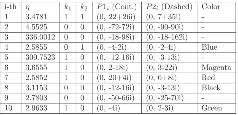
Following the theoretical construction developed in Section 5, for the two-complex dimensional case and L= 2, the input elements hm1, hm2 of the func-tional (5.7) are uniformly distributed random numbers. Also we randomly generate the values of the SNR ρ for each computational experiment i, where i= 1,2, . . . ,10. Thereby we compute the values of η in the second column of Table ??. Therefrom the functional (5.7) and its respective quadratic form is obtained. The minimum of the equation (5.8) corresponds to ab∈Λ′such that bis the closest lattice point to the origin.
For each computational experiment i, we find the vector a∈ (Z[i]4− {0}) which gives us the best estimation for the respective equations in (5.4). In (5.4) we have
(1 +ξ8)k1 =a10+a11ξ8 (a)
(1 +ξ8)k2 =a20+a21ξ8 (b), (5.9) where (a) and (b) correspond, respectively, to the best estimation of the quan-tizations Mk′1 and Mk′2. Each kl, where l = 1,2, is computed by taking the
closest integer of the following value
logkhmlk
logk1 +ξ8k (5.10)
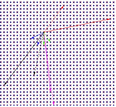
and, after that, we compute such an integer value mod 2 to obtainkl. In Figure
2 each lattice is represented by either Λ0 =Z[i]2 (blue dots) or Λ1 =D4 (red crosses).
The corresponding estimations forhm1x1 andhm2x2 are represented in Ta-ble ??by the vectors P1i and P2i, respectively, for the computational
experi-ments i= 1, . . . ,10. These estimations are points of the lattices related to the powers k1 and k2, respectively, and are associated to a coset of such lattices with (1 +i)Z[i]2 being the corresponding sublattice. Consequently, we have an efficient decoder for such a two-complex dimensional channel quantization and the corresponding achievable computation rate at each node is maximized.
pointsP1i (continous) andP2i (dashed) are estimations forhm1x1 andhm2x2, respectively.
From the computational experiments, we observe that we obtain a two-dimensional hyperplane by taking the values ofhm1 andhm2such that||hm1||= ||hm2|| = 1. We can generate such a two-dimensional hyperplane through the projection of the last complex coordinate.
i-th η k1 k2 P1i (Cont.) P2i (Dashed) Color
1 3.4781 1 1 (0, 22+26i) (0, 7+35i) -2 4.5525 0 0 (0, -72-72i) (0, -90-90i) -3 336.0012 0 0 (0, -18-98i) (0, -18-162i) -4 2.5855 0 1 (0, -4-2i) (0, -2-4i) Blue 5 300.7523 1 0 (0, -12-16i) (0, -3-13i)
-6 3.6555 1 0 (0, 2-18i) (0, 3-22i) Magenta
7 2.5852 1 0 (0, 20+4i) (0, 6+8i) Red
8 3.1153 0 0 (0, -12-16i) (0, -3-13i) Black 9 2.7803 0 0 (0, -50-66i) (0, -25-70i)
-10 2.9633 1 0 (0, -4i) (0, 2-3i) Green
Table 1: Data from the Computational Experiments
6. Conclusion
This work presents a new algebraic methodology to quantize complex-valued channels in order to realize interference alignment (IA) [1] onto a complex ideal lattice. Such a methodology makes use of the binary cyclotomic field Q(ξ2r), where r≥3, to provide a doubly infinite nested lattice partition chain for any dimensionn= 2r−2, wherer ≥3, in order to quantize complex-valued channels onto these nested lattices.
We prove the existence of periodicity in the corresponding nested lattice partition chains to guarantee that the channel gain does not remove the lattice from the initial chain of nested complex ideal lattices.
Precoding is essential to ensure onto which lattice a given complex-valued channel must be quantized. Therefore Section 4 provides us such a precoder.
Figure 2: Representation of the VectorsP1i and P2i from Table I.
Note that Λ1 =D4 ⊆Λ0=Z[i]2.
algebraic methodology through the two-complex dimensional channel quantiza-tion and show all the corresponding computaquantiza-tional experiments.
The proposed algebraic methodology is original and can be approached to applications such as compute-and-forward [13] and homomorphic encryption schemes.
7. Appendix 1: The lattice related to the canonical embedding of the ideal ℑk, where k= 1, is given by the lattice D2n, where
n= 2(r−2) We have Z[i]n/σ(ℑ)/D2
n and
Z[i]n=D2n∪(Dn⊕(Dn+ (1,0,0, . . . ,0)))∪
∪((Dn+ (1,0,0, . . . ,0))⊕Dn)∪((Dn+ (1,0,0, . . . ,0))⊕
⊕(Dn+ (1,0,0, . . . ,0))) =Dn2∪(D2n+ (0,1,0,0, . . . ,0))∪
Then σ(ℑ) is the union ofD2n with either
(Dn⊕(Dn+ (1,0,0, . . . ,0))),
or ((Dn+(1,0,0, . . . ,0))⊕Dn) or ((Dn+(1,0,0, . . . ,0))⊕(Dn+(1,0,0, . . . ,0))).
Observe thatℑ=ℑ2∪(ℑ2+ (1 +ξ2r)), thenσ(ℑ) =σ(ℑ2)∪σ(ℑ2+ (1 + ξ2r)) =Dn2 ∪σ(ℑ2+ (1 +ξ2r)) and we can conclude that σ(ℑ2+ (1 +ξ2r)) is equal to either (Dn⊕(Dn+ (1,0,0, . . . ,0))), or ((Dn+ (1,0,0, . . . ,0))⊕Dn) or
((Dn+ (1,0,0, . . . ,0))⊕(Dn+ (1,0,0, . . . ,0))).
We have σ(ℑ2+ (1 +ξ2r)) =σ(ℑ2) +σ(1 +ξ2r) =D2n+σ(1 +ξ2r), where σ(1 +ξ2r) = (1 +ξ2r, σ2(1 +ξ2r), . . . , σn(1 +ξ2r)) =
= (1 +ξ2r,1 +σ2(ξ2r), . . . ,1 +σn(ξ2r)),
where, in section 3.1, we have that{id=σ1, σ2, σ3, . . . , σn} is the Galois group
of the field extension Q(ξ2r)/Q(i) and id is the identity map.
Also, in section 3.1, we have that aZ[i]-basis of Z[ξ2r] is given by {1, ξ2r, ξ22r, ξ23r, . . . , ξn2r−1}=
={1, ξ2r, ξ2r−1, ξ2r−1ξ2r, ξ2
2r−1, . . . , ξ2 r−3−1 2r−1 , ξ2
r−3−1 2r−1 ξ2r} and the following matrix
M =
1 ξ2r ξ2r−1 · · · ξ2
r−3 −1 2r−1 ξ2r
1 σ2(ξ2r) σ2(ξ
2r−1) · · · σ2(ξ2
r−3
−1 2r−1 ξ2r)
1 σ3(ξ2r) σ3(ξ
2r−1) · · · σ3(ξ
2r−3
−1 2r−1 ξ2r)
..
. ... ... ... ... 1 σn(ξ2r) σn(ξ
2r−1) · · · σn(ξ
2r−3 −1 2r−1 ξ2r)
generates the complex algebraic lattice σ(Z[ξ2r]). Thus, we have
σ(1 +ξ2r) =M 1 1 0 0 0 .. . 0 =
1 +ξ2r
1 +σ2(ξ2r)
1 +σ3(ξ2r)
1 +σ4(ξ2r)
1 +σ5(ξ2r)
.. . 1 +σn(ξ2r)
Then we can conclude that
σ(ℑ2+ (1 +ξ2r)) =Dn2+ (1,1,0,0, . . . ,0) = = (Dn+ (1,0,0, . . . ,0))⊕(Dn+ (1,0,0, . . . ,0))
and
σ(ℑ) =Dn2 ∪((Dn+ (1,0,0, . . . ,0))⊕(Dn+ (1,0,0, . . . ,0))) =D2n.
Therefore, for r ≥ 3 and k = 1, we have the lattice D2n whose position
compared to the Z[i]n-lattice is equal tok= 1.
8. Appendix 2: Extension by periodicity of the nested lattice partition chain for the positive positions, that is, k≥0 In section 3.2, we have the lattices Λj, where 0 ≤ j ≤ n−1 and Λj is the
lattice related to the positionj. Also we have thatM(1+ξ2r)j = (M(1+ξ 2r))
j is a
generator matrix of the lattice Λj and we know that the matrices (M(1+ξ2r))n and (1+i)In×nare equivalent matrices, whereIn×nis then×nidentity matrix.
Then, fork=n, the matrix (M(1+ξ2r))
ngenerates the lattice (1+i)Z[i]n; for
k=n+j, we haveM(1+ξ
2r)(n+j) = (M(1+ξ2r))
(n+j)= ((M
(1+ξ2r))
n)(M
(1+ξ2r))
j =
(1+i)(M(1+ξ2r))j as being a generator matrix of the lattice (1+i)Λj and, fork=
2n+j, we haveM(1+ξ
2r)(2n+j) = (M(1+ξ2r))(2n+j) = ((M(1+ξ2r))2n)(M(1+ξ2r))j = (1 +i)2(M(1+ξ2r))j = 2(M(1+ξ2r))j as being a generator matrix of the lattice 2Λj, since the matrices (M(1+ξ2r))
n and (1 +i)I
n×nare equivalent.
Then we suppose, by hypothesis of induction, that (M(1+ξ2r))
nβ+j, where
β ∈Nand 0≤j≤n−1, is a generator matrix of the lattice (1 +i)βΛj.
We show, fork=n(β+ 1) +j, that the lattice (1 +i)β+1Λ
j has a generator
matrix as being the matrix (M(1+ξ2r))
(n(β+1)+j). In fact, (M
(1+ξ2r))
n(β+1)+j =
((M(1+ξ2r))n)((M(1+ξ2r))
(nβ+j)), by using the hypothesis of induction and the fact that (1 + i)In×n and (M(1+ξ2r))
n are equivalent matrices, we have
(M(1+ξ2r))n(β+1)+j as a generator matrix of the lattice (1 +i)β+1Λj.
Hence, we show, fork=nβ+j, where β ∈Nand 0≤j≤n−1, that the matrix (M(1+ξ2r))nβ+j is a generator matrix of the lattice (1 +i)βΛj.
Therefore, if β is even, we have β = 2ǫ, where ǫ ∈ N, and (1 +i)βΛ
j =
2β/2Λj, for β 6= 0; forβ = 0, we have the lattice Λj. Now ifβ is odd, we have
β = 2ǫ+ 1, whereǫ∈N, and (1 +i)βΛ
9. Appendix 3: The minimum Hamming distance dk of the code Ck,
where k= 1,2, . . . , n−1 = 2r−2−1, is even and d
k≥2
We have thatC0 is the universal codeFn2 ={0,1}n and its generator matrix is given by the matrixMC0 whose rows are the rows 0,1,2, . . . , n−1 of the Pascal’s triangle modulo 2 [11] filled by zeros to obtainncoefficients. We also know that the matrix MC1 generates the code C1 whose rows are the rows 1,2, . . . , n−1 of the Pascal’s triangle modulo 2 filled by zeros to obtainncoefficients, that is, are the rows fromMC0 by removing the first one (row 0 of the Pascal’s triangle). We show, for anyr≥3 (n= 2r−2 and k= 1,2, . . . , n−1), that the rows of the matrix MC1 have an even number of 1’s and, at least, two 1’s. In fact, for r= 3 (n= 2 andk= 1), the rows of the matrix MC1 are given by the rows 1,2 of the Pascal’s triangle modulo 2 filled by zeros to obtain 2 coefficients and we can see that these rows have an even number of 1’s and, at least, two 1’s. So dk ≥2 and is even.
For r = 4 (n = 4 and k = 1,2,3), the rows of the matrix MC1 are given by the rows 1,2,3 of the Pascal’s triangle modulo 2 filled by zeros to obtain 4 coefficients and we can see that these rows have an even number of 1’s and, at least, two 1’s. Sodk≥2 and is even.
In [11] we have the following basic properties of the Pascal’s triangle modulo 2:
1) Row 2ϑ−1 consists of 2ϑ ones: 111...111 (2ϑ 1’s);
2) Row 2ϑ consists of two ones separated by 2ϑ−1 zeros: 100...001 ((2ϑ−1)
0’s);
3) More generally, row 2ϑ+u, where 0≤u <2ϑ, consists of two copies of the rowu separated by (2ϑ−1−u) zeros.
Forr = 4 we already know that the rows 1,2,3 have an even number of 1’s and, at least, two 1’s. Observe thatr=ϑ+ 3 and then ϑ= 2. By Property 2) we have that the row 4 consists of two 1’s separated by 3 zeros and, by Property 3), we have that the rows 4 +u, where 1≤u≤3, consist of 2 copies of the row u (u= 1,2,3) separated by 3−u zeros.
Since the rowsu= 1,2,3 have an even number of 1’s and, at least, two 1’s, by Property 3) the rows 5,6,7 have an even number of 1’s and, at least, four 1’s. So the rows 1,2,3,4,5,6,7 have an even number of 1’s and, at least, two 1’s (row 4).
Hence, by using these three properties, we prove it by induction. Letr≥3, r = ϑ+ 3, k = 1,2,3, . . . , n −1 = 2r−2 −1 and the rows 2ϑ +u, where
number of 1’s and, at least, two 1’s.
Now we show, by induction, that this is valid forr+ 1 =ϑ+ 4 = (ϑ+ 1) + 3. So, for r+ 1, we have Property 3) given by the rows 2ϑ+1+u, where 0≤u≤ 2ϑ+1−1, which consist of two copies of the row u separated by 2ϑ+1−1−u zeros and we have the rows 1,2,3, . . . ,2ϑ+1−1,2ϑ+1,2ϑ+1+ 1, . . . ,2ϑ+2−1 that generate the codeC1 related tor+ 1.
However, by hypothesis of induction, we have that the rows 1,2,3, . . . ,2ϑ,2ϑ+ 1, . . . ,2ϑ+1−1 have an even number of 1’s and, at least, two 1’s and since the rows 2ϑ+1 +u, where 0 ≤ u ≤ 2ϑ+1−1, consist of two copies of the row u separated by 2ϑ+1 −1 −u zeros, it follows that the rows 1,2,3, . . . ,2ϑ+1 − 1,2ϑ+1,2ϑ+1+ 1, . . . ,2ϑ+2−1 have an even number of 1’s and, at least, two 1’s (row 2ϑ+1).
Then we prove, by induction, thatdk is even anddk ≥2.
10. Appendix 4: Providing an expression for the corresponding mean square error
From equation (1.1), we have
B−→ym= L
X
l=1
B(hmlI)−→xl+B−→zm =
=
L
X
l=1
Mk′l−→xl+ L
X
l=1
(B(hmlI)−Mk′l) − →x
l+B−→zm,
where Mk′l−→xl =Mk′l(M0 − →v
l) =M0(M(1+ξ2r)kl − →v
l), withM(1+ξ2r)kl ∈Mn(Z[i]). Hence
L
X
l=1
Mk′l−→xl = L
X
l=1
M0(M(1+ξ2r)kl−→vl) =M0
L
X
l=1
(M(1+ξ
2r)kl−→vl). We also have that
L
X
l=1
(B(hmlI)−Mk′l) − →x l = L X l=1
((M0M0H)hmlB−Mk′l) − →x l= = L X l=1
((M0M0H)hmlB)−→xl− L
X
l=1
=
L
X
l=1
(M0M0H)hmlB(M0M0H)−→xl− L
X
l=1
M0(M(1+ξ2r)kl − →v
l) =
=
L
X
l=1
(M0M0H)hmlBM0−→vl− L
X
l=1
M0(M(1+ξ2r)kl−→vl) =
=M0
L
X
l=1
(M0HhmlBM0)−→vl
! −M0
L
X
l=1 M(1+ξ
2r)kl − →v
l=
=M0
L
X
l=1
(hml(M0HBM0)−M(1+ξ2r)kl)−→vl
and B−→zm =M0(M0HB−→zm).
Then we conclude that − →y′
m =M0HB−→ym= L
X
l=1 M(1+ξ
2r)kl − →v l+ + L X l=1
(hml(M0HBM0)−M(1+ξ2r)kl)−→vl+M0HB−→zm,
where −→υm = PLl=1(hml(M0HBM0)−M(1+ξ2r)kl) − →v
l +M0HB−→zm is the noise
term (−→υm is ann×1 column vector). Thus the mean square error is given by
E[−→υHm−→υm] =T r(E[−→υHm−→υm]) =
=E[T r(−→υHm→−υm)] =E[T r(−→υm−→υHm)] =T r(E[−→υm−→υHm]) and
T r(E[−→υm−→υHm]) =
=T r(E[(
L
X
l=1
(hml(M0HBM0)−M(1+ξ2r)kl) − →v
·(
L
X
l=1
(hml(M0HBM0)−M(1+ξ2r)kl) − →v
l+M0HB−→zm)H]).
Since the variables −→vl and −→zm are uncorrelated, forl= 1, . . . , L, we have
E[−→υm−→υHm] = L
X
l=1
(hml(M0HBM0)−M(1+ξ2r)kl)·E[ − →v
l−→vHl ]·
·(hml(M0HBHM0)−M(1+H ξ2r)kl)+
+M0HBE[−→zm−→zHm]BHM0. Hence
E[−→υHm−→υm] =T r( L
X
l=1
(hml(M0HBM0)−M(1+ξ2r)kl)·E[ − →v
l−→vHl ]·
·(hml(M0HBHM0)−M(1+H ξ2r)kl)+
+M0HBE[−→zm−→zHm]BHM0).
Let E[−→vl−→vHl ] = Ps, for all l = 1, . . . , L, and E[−→zm−→zHm] = σ2N, where Ps
is the signal power, σ2
N is the noise variance andρ = σP2s N
is the signal-to-noise ratio (SNR). Then
E[−→υHm−→υm] =PsT r( L
X
l=1
(hml(M0HBM0)−M(1+ξ2r)kl)·
·(hml(M0HBHM0)−M(1+H ξ
2r)kl) + 1 ρM
H
0 BBHM0) =
=PsT r( L
X
l=1
−
L
X
l=1
hml[(M0HBM0)M(1+H ξ2r)kl+M(1+ξ2r)kl(M
H
0 BHM0)]+
+
L
X
l=1 M(1+ξ
2r)klM
H
(1+ξ2r)kl + 1 ρM
H
0 BBHM0). Thereby we have
E[−→υHm−→υm] =PsT r((khk2+1
ρ)M
H
0 BBHM0−
−
L
X
l=1
hml(M0HBM0)M(1+H ξ 2r)kl −
L
X
l=1
hmlM(1+ξ2r)kl(M0HBHM0)+
+
L
X
l=1
M(1+ξ2r)klM(1+H ξ2r)kl),
whereh= (hm1, hm2, . . . , hmL).
LetF =M0HBM0 (FH =M0HBHM0) and η= (khk2+ 1ρ). Then
E[−→υHm−→υm] =PsηT r(F·FH−
1 ηF
L
X
l=1
hmlM(1+H ξ2r)kl−
−1 ηF H L X l=1
hmlM(1+ξ2r)kl + 1 η
L
X
l=1 M(1+ξ
2r)klM
H
(1+ξ2r)kl) =
=PsηT r((F−
1 η
L
X
l=1
hmlM(1+ξ2r)kl)(F − 1 η
L
X
l=1
hmlM(1+ξ2r)kl)
H+ +1 η L X l=1 M(1+ξ
2r)klM
H
−1 η2(
L
X
l=1
hmlM(1+ξ2r)kl)(
L
X
l=1
hmlM(1+ξ2r)kl)
H).
Observe that F = 1ηPL
l=1hmlM(1+ξ2r)kl minimizes E[−→υHm−→υm]. Since F =
MH
0 BM0, it follows that BM0=
1 ηM0
L
X
l=1
hmlM(1+ξ2r)kl ⇔
⇔B = 1 ηM0(
L
X
l=1
hmlM(1+ξ2r)kl)M0H =
= 1 η
L
X
l=1
hml(M0M(1+ξ2r)klM0H).
Hence B = η1PL
l=1hml(M0M(1+ξ2r)klM
H
0 ) minimizes E[−→υHm−→υm] and the
mean square error is given by
PsT r( L
X
l=1 M(1+ξ
2r)klM
H
(1+ξ2r)kl−
−1 η(
L
X
l=1
hmlM(1+ξ2r)kl)(
L
X
l=1
hmlM(1+ξ2r)kl)
H) =
=Ps( L
X
l=1
T r(M(1+ξ 2r)klM
H
(1+ξ2r)kl)− 1 η k
L
X
l=1
hmlM(1+ξ2r)kl k 2
F) =
=Ps( L
X
l=1
kM(1+ξ 2r)kl k
2 F − 1 η k L X l=1
hmlM(1+ξ2r)kl k 2
F),
with k A kF=
p
T r(AAt), where A is an m×n complex matrix. The norm
k · kF is called Frobenius norm.
Since
kM(1+ξ
=T r(M(1+ξ 2r)klM
H
(1+ξ2r)klM0HM0) = =T r(M0M(1+ξ2r)klM(1+H ξ2r)klM
H
0 ) =
=
n
X
i=1
σi((1 +ξ2r)kl)2 =
n
X
i=1
σi(((1 +ξ2r)kl)2) =
=T rQ(ξ2r)/Q(i)(((1 +ξ2r)kl)2) and
k
L
X
l=1
hmlM(1+ξ2r)kl k2F=T r(( L
X
l=1
hmlM(1+ξ2r)kl)(
L
X
l=1
hmlM(1+ξ2r)kl)H) =
=T r(M0(
L
X
l=1
hmlM(1+ξ2r)kl)(
L
X
l=1
hmlM(1+ξ2r)kl)HM0H) =
=T r((
L
X
l=1
hmlM0M(1+ξ2r)kl)(
L
X
l=1
hmlM(1+H ξ2r)klM0H)) =
=
L
X
l,j=1
hmlhmjT rQ(ξ2r)/Q(i)((1 +ξ2r)
kl(1 +ξ2r)kj),
the mean square error is given by Ps(
L
X
l=1
T rQ(ξ2r)/Q(i)(((1 +ξ2r)kl)2)−
−1 η
L
X
l,j=1
hmlhmjT rQ(ξ2r)/Q(i)((1 +ξ2r)
kl(1 +ξ2r)kj)) =
=Ps
1 η(η
L
X
l=1
T rQ(ξ2r)/Q(i)(((1 +ξ2r)
kl)2)−
−
L
X
l,j=1
hmlhmjT rQ(ξ2r)/Q(i)((1 +ξ2r)
Acknowledgment
This work has been supported by the following Brazilian Agencies: FAPESP (Funda¸c˜ao de Amparo `a Pesquisa do Estado de S˜ao Paulo) under grants No. 2013/03976-9 and 2013/25977-7, CAPES (Coordena¸c˜ao de Aperfei¸coamento de Pessoal de N´ıvel Superior) under grant No. 6562-10-8 and CNPq (Con-selho Nacional de Desenvolvimento Cientfico e Tecnolgico) under grant No. 303059/2010-9.
References
[1] J. Tang and S. Lambotharan, Interference alignment techniques for MIMO multi-cell interfering broadcast channels, IEEE Trans. on Communica-tions,61 (2013), 164-175.
[2] A.R. Calderbank and N.J.A. Sloane, New trellis codes based on lattices and cosets, IEEE Trans. on Information Theory,33 (1987), 177-195. [3] G.D. Forney, Coset Codes - Part I: Introduction and geometrical
clas-sification, IEEE Transactions on Information Theory, 34, No 5 (1998), 1123-1151.
[4] R. Zamir, Lattices are everywhere, In: Proc. 4th Annual Workshop on Information Theory and its Applications (ITA)(2009).
[5] X. Giraud, E. Boutillon and J-C. Belfiore, Algebraic tools to build mod-ulation schemes for fading channels, IEEE Transactions on Information Theory, 43, No 3 (1997), 938-952.
[6] J. Leech and N.J.A. Sloane, Sphere packings and error correcting codes, Canadian J. of Mathematics, 23(1971), 718-745.
[7] E. Bayer-Fluckiger, F. Oggier and E. Viterbo, Algebraic lattice constella-tions: bounds on performance, IEEE Trans. on Information Theory, 52, No 1 (2006), 319-327.
[8] S. Lang,Complex Multiplication, Springer-Verlag, New York (1983). [9] C.C. Trinca, J.-C. Belfiore, E.D. de Carvalho and J. Vieira Filho, Coding
[10] C.C. Trinca, J.-C. Belfiore, E.D. de Carvalho and J. Vieira Filho, Con-struction of nested 4-dimensional complex lattices in order to realize in-terference alignment onto a lattice, In: 6th Internat. Multi-Conference on Complexity, Informatics and Cybernetics (IMCIC 2015) (2015).
[11] B.R. Hodgson, On some number sequences related to the parity of binomial coefficients,Universit´e Laval, Qu´ebec G1K 7P4, Canada,30, No 1 (1990), 35-47.
[12] K. Conrad, Dirichlet’s unit theorem, Retrieved from:
http://www.math.uconn.edu/ kconrad/blurbs/gradnumthy/unittheorem.pdf. [13] B. Nazer and M. Gastpar, Compute-and-forward: Harnessing interference