The Instinctive Outline towards Online Shortest Path
T.Chandana Gouri,Assistant Professor in CSE,
Indo American Institutions Technical Campus, Anakapalle [email protected]
ABSTRACT
Processing the most limited way between two given areas in a road network is a critical issue that discovers applications in different guide administrations and business route items. The best in class answers for the issue can be isolated into two classifications: spatial-rationality based strategies and vertex-significance based methodologies. The two classes of procedures, be that as it may, have not been thought about deliberately under the same exploratory structure, as they were created from two free lines of examination that don't allude to each other. This renders it troublesome for an expert to choose which network ought to be received for a particular application. Moreover, the exploratory assessment of the current procedures, as introduced in past work, misses the mark in a few perspectives. A few strategies were tried just on little road networks with up to one hundred thousand vertices; some methodologies were assessed utilizing separation inquiries (rather than most limited way questions), in particular, inquiries that approach just for the length of the briefest way; a cutting edge strategy was inspected in view of a defective execution that prompted mistaken inquiry results. To address the above issues, this paper exhibits a far reaching examination of the most progressive spatial-intelligence based and vertex-significance based methodologies. Utilizing an assortment of genuine road networks with up to twenty million vertices, we assessed every strategy as far as its preprocessing time, space utilization, and inquiry productivity (for both most brief way and separation questions). Our exploratory results uncover the qualities of various networks, taking into account which we give rules on selecting fitting strategies for different situations. Keywords—Shortest path, broadcasting, LTI, Road traffic, Road Networking
I. Introduction
Most concise way count is a vital limit in front line auto course networks .This limit safeguards a driver to comprehend the best course from his energy position to destination. Normally, the most constrained way is handled by detached from the net
International Journal of Science Engineering and Advance Technology,
IJSEAT, Vol. 4, Issue 8
ISSN 2321-6905
August -2016
correspondence cost will be spent on sending result routes on the model. Plainly, the client server basic designing will soon get the opportunity to be nonsensical in overseeing enormous live development in not all that inaccessible future. Client server basic building, it can't scale well with a broad number of customers. Besides, reported ways are inaccurate results and the network does not give any exactness guarantee. An alternative course of action is to broadcast live action data over remote framework (e.g., 3G, LTE, Mobile WiMAX, et cetera.). The course network gets the live movement data from the broadcast station and executes the computation by local norms (called rough transmission model). The development data are appeared by a game plan of groups for each broadcast cycle. To answer briefest path questions in light of live development circumstances, the course network must get those overhauled packages for each show cycle. The guideline challenge on noticing live most constrained ways is versatility, to the extent the amount of clients and the measure of live development upgrades. Another and promising response for the most constrained way computation is to demonstrate an air list over the remote framework (called list transmission model). The essential central purposes of this model are that the framework overhead is free of the amount of clients and every client just downloads an entire's section guide as demonstrated by the document information. For instance, the proposed list constitutes a course of action of pairwise slightest and most amazing voyaging costs between every two sub-portions of the aide. Regardless, these schedules simply settle the versatility issue for the amount of clients however not for the measure of live action overhauls. As reported the re estimation time of the rundown takes 2 hours for the San Francisco (CA) guide. It is prohibitively extravagant to overhaul the record for OSP, to stay mindful of live action circumstances. Convinced by the nonattendance of off-the-rack answer for OSP, Anew course of action in perspective of the record transmission model by introducing live movement document (LTI) as the middle strategy. LTI is required to give for the most part short tune-in cost (at client side), snappy request response time (at client side), little show size (at server side), and light bolster time (at server side) for OSP. LTI highlights as takes after. • The record structure of LTI is updated by two novel methods, graph distributing stochastic-based improvement, in the wake of driving a serious examination on the different leveled list networks. To the best of our understanding, this is the primary work to give a thorough cost examination on
the different leveled record strategies and apply stochastic methodology to streamline the document dynamic structure. • LTI adequately keeps up the record for live development circumstances by merging Dynamic Shortest Path Tree (DSPT) into dynamic rundown networks. • LTI diminishes the tune-in cost up to a solicitation of degree when diverged from the best in class contenders; while notwithstanding it gives centered request response time, broadcast size, and bolster time. To the best of our knowledge, we are the main work that tries to minimize all these execution components.
II. Related Work
concerning static quickest way issues. In any case, Halpern [13] demonstrated that the speculation of Dijkstra's calculation is valid for FIFO networks. On the off chance that the FIFO property does not hold in a period subordinate network, then the issue is NP-Hard. In [14], Orda and Rom presented Bellman-Ford based calculation where they decide the way toward destination by refining the landing time capacities on every hub in the entire time interim T. In [15], Kanoulas et al. proposed Time Interval All Fastest Path (allFP) approach in which they keep up a need line of all ways to be extended as opposed to sorting the need line by scalar qualities. They specify every one of the ways from source to a destination hub which causes exponential running time in the most pessimistic scenario. In [16], Ding et al. utilized a variety of Dijkstra's calculation to take care of the TDFP issue. With their TDFP calculation, utilizing Dijkstra like extension, they decouple the way determination and time refinement (registering most punctual landing time capacities for hubs) for a given beginning time interim T. Their calculation is additionally appeared to keep running in exponential time for unique cases [17]. The center of both [15] and [16] is to locate the speediest way in time subordinate road networks for a given begin time interim. The ALT calculation [18] was initially proposed to quicken speediest way calculation in static road networks. With ALT, an arrangement of hubs called points of interest are picked and after that the most limited separations between every one of the hubs in the network and every one of the historic points are registered and put away. ALT utilizes triangle disparity in light of separations to the milestones to get a heuristic capacity to be utilized as a part of A* inquiry. The time subordinate variation of this procedure is examined in [19] (unidirectional) and [20] (bidirectional A* look) where heuristic capacity is registered w.r.t lowerbound chart. Be that as it may, the historic point choice is exceptionally troublesome and the measure of the pursuit space is extremely influenced by the decision of milestones. So far no ideal methodology regarding point of interest determination and irregular inquiries has been found. In particular, historic point determination is NP-hard [21] and ALT does not ensure to yield the littlest inquiry spaces as for quickest way calculations where source and destination hubs are picked aimlessly. Our examinations with genuine time subordinate travel-times demonstrate that our methodology devours considerably less capacity when contrasted with ALT based methodologies and yields quicker reaction times. In two diverse studies, The Contraction Hierarchies (CH) and SHARC
techniques (likewise created for static networks) were enlarged to time-subordinate road networks in [8] and [9], individually. The fundamental thought of these networks is to expel irrelevant hubs from the diagram without changing the quickest way removes between the staying (more vital) hubs. Be that as it may, not at all like the static networks, the significance of a hub can change for the duration of the time under thought in time subordinate networks, thus the significance of the hubs are time shifting. Considering the polynomial info size, and henceforth the super-polynomial number of critical hubs with time-subordinate networks, the fundamental deficiencies of these methodologies are illogical pre-handling times and broad space utilization. For instance, the precomputation time for SHARC in time subordinate road networks takes over 11 hours for moderately little road networks (e.g. LA with 304,162 hubs) [9]. Additionally, because of the huge utilization of curve banners [9], SHARC does not work in a dynamic situation: at whatever point an edge cost capacity changes, circular segment banners ought to be recomputed, despite the fact that the diagram parcel need not be upgraded. While CH additionally experiences moderate pre-handling times, the space utilization for CH is no less than 1000 bytes for each hub for less fluctuated edge-weights where the capacity cost increments with certifiable time-subordinate edge weights. In this manner, it may not be plausible to apply SHARC and CH to mainland size road networks which can comprise of more than 45 million road portions (e.g., North America road network) with perhaps extensive changed edge weights.
III. Problem Statement
The briefest way calculation is mostly utilized as a part of the road network. The primary arrangement of the ideal course inquiry depends on the pre-put away weights. The principal approaches considered just the end focuses. A large portion of the methods have impediments in some specific territory. The principle issues are to discover briefest way amid road movement networks. Among this some may consider requirements and others without consider the imperatives and these are the fundamental issues to consider.
IV. Traffic Database
International Journal of Science Engineering and Advance Technology,
IJSEAT, Vol. 4, Issue 8
ISSN 2321-6905
August -2016
framework, for example, the one used to screen the San Francisco Bay Area traffic conditions 2 , can utilize radiofrequency labels set in every auto to track the ways navigated by individual vehicles. These labels can be the same ones utilized for robotized toll gathering, the city would simply introduce perusers at numerous non-toll roads. For this situation, every movement perception will be of the structure (auto id, edge id, time, speed), where auto id is a vehicle identifier, and different qualities are characterized as some time recently. Vehicle-level perceptions can be sorted on auto id and t to produce a way database, where every passage is the succession of edges crossed by an auto amid a driving session. We can utilize either type of information to decide continuous driving examples. On the off chance that just edge-level information is accessible, we can utilize the quantity of edge perceptions as backing, however for this situation just continuous length-1 examples can be mined. In the event that we have vehicle-level information, we can mine more drawn out successive driving examples. Notwithstanding speed data at every edge, we can expand the movement database with the arrangement of driving conditions present amid every edge perception. Given an arrangement of accessible driving elements D1, . . . ,Dn, we can enlarge every traffic perception with the tuple (d1, . . . , dn) where each di is a worth for driving variable Di. Table 3 displays a case movement database in way arrange, where every way stage is of
car id path ((edge id, start time, end time), . . . ) 1 (e1, 10, 15)(e2, 15, 23)(e7, 23, 29) 2 (e3, 20, 29)(e1, 29, 33)
3 (e1, 9, 16)(e2, 16, 22)
4 (e9, 10, 11)(e2, 11, 17)(e8, 17, 20) . . . .
Table 2: Traffic Database
The form (edge id, start time, end time), where start time is the time when the car entered the edge, and end time is the time when the car exited the edge. For lack of space we do not show observed driving conditions at path stages. In the above example we have that support(e1) = 3, support(e2) = 3, support(e7) = 1, etc.
V. ROAD NETWORK PARTITIONING Road Hierarchy
Road networks are sorted out around an all around characterized pecking order of roads. A case of a run of the mill road progressive network is the road network of the United States, where thruways associate different expansive districts, interstate roads interface areas inside a locale, multi-path roads interface city territories, and little roads venture into individual houses. Data on road classifications is
can build a progression of ranges as a tree of profundity l − 1: The root hub speaks to the whole road network, offspring of the root hub speak to the zones shaped by apportioning the root utilizing level-1 edges, the hubs in every territory frame a diagram themselves, and all the edges from E interfacing two hubs in a region are said to have a place with the region. A hub at level-k results from the allotment of its guardian hub utilizing the edges of class k − 1. Notice that as per this tradition, road class 1 is the biggest, and road class l the littlest.
Area partitioning algorithm
In this area we build up a proficient calculation that can consequently create a semantically significant parcel of the road network by utilizing road progression data. The calculation utilizes a surge filling method to recognize emphatically associated parts delimited by abnormal state edges. We take as info the road network G and the edge class k utilized for dividing. Clench hand we dole out to every hub a void arrangement of regions. We then pick a hub n with class(n) > k (i.e., associated with edges less vital than the ones utilized for dividing), and add territory a to this present hub's range set; as of right now we move to all neighbors of the hub that are reachable through the edges of the classes more prominent than k, and add a to their region sets. This procedure rehashes until no further hubs can be come to. We are essentially strolling in each conceivable heading from the hub until we achieve vast roads utilized for dividing and we stop. Right now we expand our territory number, move to the tracking hub with a void region set, and rehash the procedure until all hubs are relegated to no less than one range. One
pleasant component of the calculation is that it consequently distinguishes inside hubs (those with a solitary zone in their general vicinity set), and outskirt hubs (those with various zones in their general vicinity set). Investigation. Calculation 1 looks at every inside hub O(1) times, and fringe hubs O(|a|), where |a| is the quantity of regions. So the request of the general calculation is O(n× |a|). When all is said in done, |a| ¿ n. So the calculation can be viewed as straight in the quantity of hubs. In our trials we divided genuine road network charts with more than a million hubs in only a few moments.
Algorithm 1 Area partitioning
Input: G(V, E), k edge class used to partition G. Output: Partition P(k) = V1k, V2k,………, Vnk Method:
1: area = 0;
2: Areas[ni] = φ for all node ni; 3: for Each node ni do
4: if Area[ni] = φ and class(ni) > k then 5: q.push(ni);
6: while not q.empty() do 7: n← q.pop(); n.mark = true; 8: Area[n] = Area[n] S{area};
9: push into q all neighbors of n reachable through edges of class greater than k, s.t., n.mark = false; 10: end while
11: area = area + 1; 12: q.clear(); 13: end if 14: end for
15: for each area i construct ViK
as the set of nodes n such that i∈Area[n]
VI. Proposed Work
We propose a bidirectional time subordinate quickest way calculation (BTDFP) based on A* seek [2]. There are two fundamental difficulties to utilize bidirectional A* seek in time subordinate networks. To begin with, finding an allowable heuristic capacity (i.e., lower bound separation) between a middle of the road vi hub and the destination d is trying as the separation between viand d changes in light of the flight time from vi . Second, it is impractical to execute a regressive hunt without knowing the landing time at the destination. We address the previous test by dividing the road network to non-covering segments (a disconnected from the net operation) and precompute the intra (hub to-fringe) and bury (outskirt to-outskirt) segment separation marks as for Lower-bound Graph G which is created by substituting the edge travel times in can build a progression of ranges as a tree of
profundity l − 1: The root hub speaks to the whole road network, offspring of the root hub speak to the zones shaped by apportioning the root utilizing level-1 edges, the hubs in every territory frame a diagram themselves, and all the edges from E interfacing two hubs in a region are said to have a place with the region. A hub at level-k results from the allotment of its guardian hub utilizing the edges of class k − 1. Notice that as per this tradition, road class 1 is the biggest, and road class l the littlest.
Area partitioning algorithm
In this area we build up a proficient calculation that can consequently create a semantically significant parcel of the road network by utilizing road progression data. The calculation utilizes a surge filling method to recognize emphatically associated parts delimited by abnormal state edges. We take as info the road network G and the edge class k utilized for dividing. Clench hand we dole out to every hub a void arrangement of regions. We then pick a hub n with class(n) > k (i.e., associated with edges less vital than the ones utilized for dividing), and add territory a to this present hub's range set; as of right now we move to all neighbors of the hub that are reachable through the edges of the classes more prominent than k, and add a to their region sets. This procedure rehashes until no further hubs can be come to. We are essentially strolling in each conceivable heading from the hub until we achieve vast roads utilized for dividing and we stop. Right now we expand our territory number, move to the tracking hub with a void region set, and rehash the procedure until all hubs are relegated to no less than one range. One
pleasant component of the calculation is that it consequently distinguishes inside hubs (those with a solitary zone in their general vicinity set), and outskirt hubs (those with various zones in their general vicinity set). Investigation. Calculation 1 looks at every inside hub O(1) times, and fringe hubs O(|a|), where |a| is the quantity of regions. So the request of the general calculation is O(n× |a|). When all is said in done, |a| ¿ n. So the calculation can be viewed as straight in the quantity of hubs. In our trials we divided genuine road network charts with more than a million hubs in only a few moments.
Algorithm 1 Area partitioning
Input: G(V, E), k edge class used to partition G. Output: Partition P(k) = V1k, V2k,………, Vnk Method:
1: area = 0;
2: Areas[ni] = φ for all node ni; 3: for Each node ni do
4: if Area[ni] = φ and class(ni) > k then 5: q.push(ni);
6: while not q.empty() do 7: n← q.pop(); n.mark = true; 8: Area[n] = Area[n] S{area};
9: push into q all neighbors of n reachable through edges of class greater than k, s.t., n.mark = false; 10: end while
11: area = area + 1; 12: q.clear(); 13: end if 14: end for
15: for each area i construct ViK
as the set of nodes n such that i∈Area[n]
VI. Proposed Work
International Journal of Science Engineering and Advance Technology,
IJSEAT, Vol. 4, Issue 8
ISSN 2321-6905
August -2016
Gwith least conceivable travel-times. We utilize the blend of intra and entomb separation names as a heuristic capacity in the online calculation. To address the last test, we run the regressive hunt on the lower-bound diagram (G) which empowers us to channel in the arrangement of the hubs that should be investigated by the forward inquiry. We clarify our bidirectional time subordinate speediest way approach that we sum up bidirectional A* calculation proposed for static spatial networks [26] to time subordinate road networks. Our proposed arrangement includes two stages. At the precomputation stage, we parcel the road network into non-covering segments and precompute lower-bound separation names inside and over the segments as for G(V,E). Progressively, at the online stage, we utilize the pre-registered separation names as a heuristic capacity in our bidirectional time subordinate A* look that performs concurrent quests from source and destination. As appeared in [5], the time subordinate speediest way issue can be unraveled by adjusting Dijkstra calculation. We allude to adjusted Dijkstra calculation as time ward Dijkstra (TD-Dijkstra). TD-Dijkstra visits all network hubs reachable from s in each course until destination hub d is come to. On the other side, a period subordinate A* calculation can essentially lessen the quantity of hubs that must be crossed in TD-Dijkstra calculation by utilizing a heuristic capacity h(v) that coordinates the hunt towards destination. To ensure ideal results, h(v) must be permissible and reliable (a.k.a, monotonic). The suitability infers that h(v) must be not exactly or equivalent to the real separation amongst v and d. With static road networks where the length of an edge is steady, Euclidian separation amongst v and d is utilized as h(v). Be that as it may, this basic heuristic capacity can't be straightforwardly connected to time-subordinate road networks, on the grounds that, the ideal travel-time amongst v and d changes in view of the takeoff time television from v. In this manner, in time-subordinate road networks, we have to utilize an estimator that never overestimates the travel-time amongst v and d for any conceivable television. One straightforward lowerbound estimator is deuc(v, d)/max(speed), i.e., the Euclidean separation amongst v and d isolated by the most extreme rate among the edges in the whole network. In spite of the fact that this estimator is ensured to be a lower-bound, it is a free bound, and consequently yields immaterial pruning. With our methodology, we get a much more tightly bound by using the pre processed separation marks. Expecting that an online time subordinate speediest way question asks for a way from source s
in parcel Si to destination d in segment S. The speediest way should go through from one outskirt hub bi in Si and another fringe hub bj in Sj . We realize that the time-subordinate quickest way remove going from bi and bj is more prominent than or equivalent to the pre figured lower-bound outskirt to-fringe (e.g., LTT (bl ,bt)) separation for Si and Sj pair. We likewise realize that a time dependent quickest way separate from s to bi is constantly more noteworthy than or equivalent to the precomputed lower-bound speediest way separation of s to its closest fringe hub bs . Comparably, same is valid from the fringe hub bd(i.e., closest outskirt hub) to noise Sj . In this way, we can register a lower-bound estimator of s by h(s) = LTT (s, bs) + LTT (bl ,bt) + LTT (bd, d).
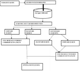
Fig. Proposed System Architecture Algorithm 1.B-TDFP Algorithm
1. Input: GT,G, s:source, d:destination,ts:departure time
2. Output: a (s, d, ts) fastest path
3. FS():forward search, BS():backward search, Nf/Nb: nodes scanned by FS()/BS(),dbv:label of the minimum element in BS queue
4. FS(GT ) and BS(G) //start searches simultaneously 5. Nf← FS(GT ) and Nb← BS(G)
6. If Nf∩ Nb_=∅then u← Nf∩ Nb 7. M = TDFP(s, u, ts) + TDFP(u, d, tu) 8. end If
9. While dbv>M 10. Nb← BS(G) 11. EndWhile 12. FS(Nb) 13. return (s, d, ts) VII. CONCLUSION
We developed an adaptive fastest path algorithm, that bases routing decision on driving and speed patterns
International Journal of Science Engineering and Advance Technology,
IJSEAT, Vol. 4, Issue 8
ISSN 2321-6905
August -2016
Gwith least conceivable travel-times. We utilize the blend of intra and entomb separation names as a heuristic capacity in the online calculation. To address the last test, we run the regressive hunt on the lower-bound diagram (G) which empowers us to channel in the arrangement of the hubs that should be investigated by the forward inquiry. We clarify our bidirectional time subordinate speediest way approach that we sum up bidirectional A* calculation proposed for static spatial networks [26] to time subordinate road networks. Our proposed arrangement includes two stages. At the precomputation stage, we parcel the road network into non-covering segments and precompute lower-bound separation names inside and over the segments as for G(V,E). Progressively, at the online stage, we utilize the pre-registered separation names as a heuristic capacity in our bidirectional time subordinate A* look that performs concurrent quests from source and destination. As appeared in [5], the time subordinate speediest way issue can be unraveled by adjusting Dijkstra calculation. We allude to adjusted Dijkstra calculation as time ward Dijkstra (TD-Dijkstra). TD-Dijkstra visits all network hubs reachable from s in each course until destination hub d is come to. On the other side, a period subordinate A* calculation can essentially lessen the quantity of hubs that must be crossed in TD-Dijkstra calculation by utilizing a heuristic capacity h(v) that coordinates the hunt towards destination. To ensure ideal results, h(v) must be permissible and reliable (a.k.a, monotonic). The suitability infers that h(v) must be not exactly or equivalent to the real separation amongst v and d. With static road networks where the length of an edge is steady, Euclidian separation amongst v and d is utilized as h(v). Be that as it may, this basic heuristic capacity can't be straightforwardly connected to time-subordinate road networks, on the grounds that, the ideal travel-time amongst v and d changes in view of the takeoff time television from v. In this manner, in time-subordinate road networks, we have to utilize an estimator that never overestimates the travel-time amongst v and d for any conceivable television. One straightforward lowerbound estimator is deuc(v, d)/max(speed), i.e., the Euclidean separation amongst v and d isolated by the most extreme rate among the edges in the whole network. In spite of the fact that this estimator is ensured to be a lower-bound, it is a free bound, and consequently yields immaterial pruning. With our methodology, we get a much more tightly bound by using the pre processed separation marks. Expecting that an online time subordinate speediest way question asks for a way from source s
in parcel Si to destination d in segment S. The speediest way should go through from one outskirt hub bi in Si and another fringe hub bj in Sj . We realize that the time-subordinate quickest way remove going from bi and bj is more prominent than or equivalent to the pre figured lower-bound outskirt to-fringe (e.g., LTT (bl ,bt)) separation for Si and Sj pair. We likewise realize that a time dependent quickest way separate from s to bi is constantly more noteworthy than or equivalent to the precomputed lower-bound speediest way separation of s to its closest fringe hub bs . Comparably, same is valid from the fringe hub bd(i.e., closest outskirt hub) to noise Sj . In this way, we can register a lower-bound estimator of s by h(s) = LTT (s, bs) + LTT (bl ,bt) + LTT (bd, d).
Fig. Proposed System Architecture Algorithm 1.B-TDFP Algorithm
1. Input: GT,G, s:source, d:destination,ts:departure time
2. Output: a (s, d, ts) fastest path
3. FS():forward search, BS():backward search, Nf/Nb: nodes scanned by FS()/BS(),dbv:label of the minimum element in BS queue
4. FS(GT ) and BS(G) //start searches simultaneously 5. Nf← FS(GT ) and Nb← BS(G)
6. If Nf∩ Nb_=∅then u← Nf∩ Nb 7. M = TDFP(s, u, ts) + TDFP(u, d, tu) 8. end If
9. While dbv>M 10. Nb← BS(G) 11. EndWhile 12. FS(Nb) 13. return (s, d, ts) VII. CONCLUSION
mined from historical data. This is a radical departure from traditional algorithms that have focused only on speed and Euclidean distance considerations. The routes computed by our algorithm are not only fast given a set of driving conditions but also reflect observed driving preferences. This is in sharp contrast to existing algorithms that may send a driver through high crime areas of a city at night, or through unsafe roads in order to save a few minutes of travel time. A road network partitioning algorithm was introduced. The algorithm uses the hierarchy of roads to segment the network into areas that are enclosed by large roads. This method yields very natural partitions, where large areas are observed at regions with low road densities, and much finer areas are observed at dense regions such as big cities. Areas are a central concept to route planning, as they provide the basis for hierarchical path finding, area level precomputation, and area sensitive support of driving patterns. We showed that significant query processing gains can be obtained, by following the principle that drivers tend to travel through the largest roads available for the trip, unless small roads along the way have a speed advantage over the large ones. We also presented a method to identify such fast roads, and efficiently incorporate them into route planning. In our experimental study we demonstrated that incorporating fast small roads into the hierarchical path finding algorithm can significantly improve the quality of routes. Through an empirical study, on real road networks, using a realistic traffic information, we verify the large performance gains of our algorithms vs. competing methods, while showing that computed routes are close to optimal. REFERENCES
[1] Leong Hou U, Hong Jun Zhao, Man Lung Yiu, Yuhong Li, and Zhiguo Gong, “Towards Online Shortest Path Computation”, IEEE TRANSACTIONS ON KNOWLEDGE AND DATA ENGINEERING, VOL. 26, NO. 4, APRIL 2014 [2] A. Deepthi, Dr. P. Srinivas Rao, S. Jayaprada, Ch. UjjwalaRoopa ,”A new approach for computing shortest path for Road Networks”., International Journal of Emerging Technology and Advanced Engineering Volume 5, Issue 4, April 2015
[3] JagadeeshMailu And M. Ganthimathi, “Enhanced Online Shortest Path Using Traffic Index Approach”, International Journal of Computer Application Issue 5, Volume 1 (Jan.- Feb. 2015)
[4] R.SUBASHINI, A.JEYA CHRISTY “Online Shortest Path based on Traffic Circumstances” , International Journal of Computer Science and Mobile Computing, Vol.3 Issue.11, November- 2014, pg. 331-337
[5] MALLEPOGU VINOD KUMAR, B.SREEDHAR “LTI Shortest Path Algorithm for Virtual Network Construction of Online Shortest Path Computation” International Journal of Scientific Engineering and Technology Research Volume.04, IssueNo.12, May- 2015, Pages: 2258-2262
[6] Mr.NikhilAsolkar, Prof. Satish R. Todmal “Online Shortest Path Computation on Time Dependent Network” International Journal of Advanced Research in Computer Engineering & Technology (IJARCET) Volume 3 Issue 12, December 2014
[7] T. Buhler and M. Hein, “Spectral Clustering Based on The Graph Laplacian,” Proc. Int’l Conf. Machine Learning (ICML), p. 11, 2009.
[8] R. Bauer and D. Delling, “SHARC: Fast and Robust Unidirectional Routing,”pp. 13-26, 2008. [9] A.V. Goldberg and R.F.F. Werneck, “Computing Point to point Shortest Path from External Memory”, 2005.