AbstractThis paper derives the relationship between the static stiffness and modal stiffness of a structure. The static stiffness and modal stiffness are two important concepts in both structural statics and dynamics. Although both stiffnesses indicate the capacity of the structure to resist deformation, they are obtained using different methods. The former is calculated by solving the equations of equilibrium and the latter can be obtained by solving an eigenvalue problem. A mathematical relationship between the two stiffnesses was derived based on the definitions of two stiffnesses. This relationship was applicable to a linear system and the derivation of relationships does not reveal any other limitations. Verification of the relationship was given by using several examples. The relationship between the two stiffnesses demonstrated that the modal stiffness of the fundamental mode was always larger than the static stiffness of a structure if the critical point and the maxi-mum mode value are at the same node, i.e. for simply supported beam and seven storeys building are 1.5% and 15% respectively. The relationship could be applied into real structures, where the greater the number of modes being considered, the smaller the difference between the modal stiffness and the static stiffness of a structure.
Keywordsstatic stiffness, modal stiffness, relationship of stiffnesses, frequency, static, dynamic
I.INTRODUCTION
he stiffness of a structure is generally understood to be the ability of a structure to resist deformation. Structural stiffness describes the capacity of a structure to resist deformations induced by applied loads. If a discrete model of a structure is considered, its structural stiffness of a structure can be completely described by its stiffness matrix. However, it may be difficult to be able to sense how stiff a structure is from its stiffness matrix. In engineering practice a single value of the stiffness of a structure is preferred as it gives a direct indication of how stiff the structure is” [6]. As the static stiffness and modal stiffness are defined independently and different-ly, the values calculated from the two definitions may differ for the same structure. However, as the two values are calculated on the basis of the same structure, i.e. using the same stiffness matrix, there should be a relationship between them.
The objectives of this research are to establish the relationship between the static stiffness and modal stiff-ness of a structure and to verify this relationship into a real structure.
1Endah Wahyuni is with Department of Civil Engineering, FTSP,
Institut Teknologi Sepuluh Nopember, Surabaya, 60111, Indonesia. E-mail: [email protected].
2Tianjian Ji is with School of Mechanical, Aerospace and Civil
Engineering, The University of Manchester, PO Box 88, Manchester M60 1QD,UK. E-mail: [email protected]
II. THEORIES
The static stiffness of a structure relates to a unit load applied on the structure and can be uniquely defined. “Point stiffness is the inverse of the displacement in the load direction on a node where a unit load is applied. Thus the point stiffness relates to the position and direction where the unit load is applied; in other words, the point stiffness values at different positions and directions are different. The static stiffness of a structure in the loading direction is the smallest value among all point stiffnesses, i.e.
Ks = min {k1, k2, ..., kj, ..., kn} (1)
where Ks is the static stiffness in the load direction, kj is
the point stiffness at the j th node and n is the number of nodes of the model of the structure. Alternatively the static stiffness can be expressed as the inverse of the maximum displacement induced by a unit force at the load location and direction, i.e.
{
j n}
s
u u u u
K max , ,..., ,...,
1
2 1
= (2)
Where uj is the displacement in the load direction on the j th node where a unit force is applied. The location of
the node where the maximum displacement occurs is called the critical point. For many structures the critical point can be easily identified, for example for a hori-zontal cantilever the critical point for a vertical load will be at the end of the cantilever, or for a simply supported rectangular plate it will be at the centre of the plate, and for a plane frame supported at its base the critical point for a horizontal load will be at the top of the frame” [5].
Consider a structure that is modeled by n nodes and m elements. Each node consists of d degrees of freedom. Therefore, the static equilibrium equation, containing n x
d unknowns, is expressed as
[K] {U} = {P} (3)
Where {U} and {P} are the displacement and load vectors respectively. [K] is the stiffness matrix that includes the effect of boundary conditions and is independent of the load for linear problems. [K] thus also describes how stiff the structure is to resist external loads.
Based on the definition of the static stiffness, only a unit load is applied on the critical node and in the concerned direction, i.e.
{P} = {0, 0, …1,…,0,0}T (4)
here ε* is the equivalent transformation strain.
Solving Equation (3) leads to the solution of the dis-placement and the maximum disdis-placement at the critical point Ucl based on Equation (4). Therefore the static
stiffness of the structure, according to Equation (2), is
cl s
u
K = 1 (5)
Relationship between Static Stiffness and Modal
Stiffness of Structures
Endah Wahyuni
1and Tianjian Ji
21There are a number of ways to determine the modal stiffness of a structure, which relates to the vibration modes of the structure. Three typical methods are briefly
described below.
A. Numerical Method
The eigenvalue problem of a structure [2] is
([K] - ω2 [M]) {Φ} = 0 (6)
The eigenvalue and the eigenvectors of the structure can be obtained by solving the equation. The following relationships are true
{ }
[ ]{ }
≠ = = Φ Φ j i j i M M i j T i 0 (7){ }
[ ]{ }
≠ = = Φ Φ j i j i KK j mi
T i
0
, (8)
where Φi, Mi and Km,i are the eigenvector, modal mass
and modal stiffness of the i th mode respectively. Thus, the modal stiffness of the i th mode can be calculated by solving Equation (6) and then using Equation (8).
B. Experimental Method
The modal stiffness of the i th mode has the following relationship
Km,i = ωi2 Mi (9)
Where ωi is the natural frequency of the i th mode.
Among these natural frequencies the fundamental frequency ωi can be easily and accurately measured. The
modal mass can be calculated by using Equation (7) where the vibratory mode can either be calculated or assumed, such as using the deformation shape of the structure subjected to its self-weight.
C. Energy Method
The n x d independent vectors in [Φ] constitute a base of a n x d dimensional space. Any vector in the space can be expressed as a linear combination of the base vectors [Φ]. Thus a displacement vector [U] can be expressed as a superposition of the responses of the base vectors, i.e.
[ ]
U z{ }
[ ]{ }
Zr
i i i =Φ
=
∑
=1
φ (10)
where zi is the generalized coordinates and r equals n x d.
The total strain energy of a structural system written in a discrete form is
{ }
[ ]{ }
{ } { }
[ ]{ }{ }
{ }
[ ]{ }
∑
= = = = r i mi im T T T T z K Z K Z Z K Z U K U E 2 , 2 1 2 1 2 1 2 1 φ φ (11)
Equation (11) indicates that the total energy of a structure can be expressed as the sum of the energy of each mode. In the above derivation, Equation (8) and Equation (10) are used. The modal stiffness of the i th mode can therefore be obtained from Equation (11) by differentiating E twice in respect to the generalized coordinate zi, i.e.
2 2 , i i m z E K ∂ ∂ = (12)
Equation (12) is useful, in particular, when the strain energy of the structure system can be easily represented by using the generalized coordinates.
Substituting Equation (10) into the static equilibrium equation (Equation (3)) and pre-multiplying by
{ }
ΦTgives
[Φ]T [K] [Φ] {Z} = [Φ]T {P} or
{ } { }
{ } { }
{ } { }
= = r cl cl cl T r T T r r m m m P P P z z z K K K , 2 , 1 , 2 1 2 1 , 2 , 1 , ... ... ... ... φ φ φ φ φ φ (13) i.e.Km,i zi {φi}T {P} = Pi φcl,i i = 1, 2, ..., r (14)
where φcl,i is the value of the i th mode at the critical
point in the loading direction.
The structural response at the critical point and in the load direction is (from Equations (10) and (14))
∑
∑
∑
= = = = = = ri mi
i cl r
i mi
i cl i cl r i i i cl cl K K z u 1 , 2 , 1 , , , 1 , . φ φ φ φ (15)
According to the definition given in equation (2), equation (15) becomes
r m r cl m cl m cl m cl r
i mi
i cl
s K K K K K
K , 2 , 3 , 2 3 , 2 , 2 2 , 1 , 2 1 , 1 , 2 , ....
1 φ φ φ φ φ
+ + + + = =
∑
= (16)Equation (16) provides the relationship between the static stiffness and the modal stiffness of a structure. The relationship is applicable to any linear system and there are no other limitations given in the derivation of Equation (16).
The physical meaning of Equation (16) is that the deflection of a single spring with stiffness of Ks is equal
to that of a series of springs with stiffness’s of Km,i/φcl,i 2
(i = 2, 3, …, r) when a unit load is applied on the two systems, as shown in Fig. 1.
As φcl,i2 > 0 and Km,i > 0 (i = 2, 3, …, n), Equation (16)
becomes 1 , 2 1 , 1 m cl s K K φ
> (17)
If φcl,i =1, i.e. the point where the fundamental mode
has the maximum value (the maximum mode value) is the critical point, it leads to
Km,1 > Ks (18)
Equation (18) indicates that the modal stiffness of the fundamental mode of a linear system is always larger than the static stiffness if the critical point and the maximum mode value are at the same node.
III.METHOD
A. Analythical Verification
The basic relationships (Equations (16) and (18)) can be demonstrated by a simple supported beam, where analytical expression can be derived. Consider a simply supported beam subjected to a concentrated load P at its centre as shown in Fig. 2.
The critical point of a simply supported beam is at the centre of the beam where the vertical unit load is applied. The maximum displacement induced by the load is L3/(48.EI). Based on the definition given in Equation (3) the static stiffness for the simply supported beam is
The natural frequency of the i th mode of the simply supported beam is
4 2
2 mL
EI i
fi= π or 2 2 4
mL EI i
i π
ω = (20)
The i th mode shape of the simply supported beam is
=
L x i sin ) x ( i
π
φ (21)
The value of the
φ
cl ,i at the centre of the beam, x = L/2,is
( )
= =
0 1
2 ,
L i i
cl
φ
φ
,....
6
,
4
,
2
,....
5
,
3
,
1
=
=
i
when
i
when
(22)
The modal mass of the beam is
∫
==L i
i
mL dx ) x ( ) x ( m M
0 2
2
φ (23)
The modal stiffness of the beam can be calculated using Equations (9) as follows
4 4 4 4
2
, 4 3
2 2
m i i i
i EI mL i EI
K M
mL L
π π
ω
= = = (24)
where i = 1, 3, 5, …
Substituting the static stiffness in Equation (19) and modal stiffness of the i th mode in Equation (24) into the relationship Equation (16) leads to
3 3 3 3
4 4 4 4 4 4
3
4 4 4 4
2 2 2
0 0 ....
48 1 3 5
2 1 1 1
0 0 ...
1 3 5
L L L L
EI EI EI EI
L EI
π π π
π
= + + + + +
= + + + + +
(25)
Fig. 1. Physical representation of the relationship of the two stiffnesses
Fig.2. A simply supported beam under a concentrated load
Removing the common terms in both sides of equation (25) gives the following identical equation
4
4 4 4 4
1,3,5,...
1 1 1 1
96 1 ... 96
3 5 7 i i
π ∞
=
= + + + + =
∑
(26)
Equation (26) is known as an application of the Fourier series, which demonstrates that the relationship (Equation (16)) between the static and modal stiffness of a structure is held.
The accuracy of approximation to the maximum static displacement (the item on the left side of Equation (25)) using the modal displacement (the items on the right side of Equation (25)) is examined by considering the first few items.
The ratio of the modal stiffness of the fundamental mode (Equation (24)) to the static stiffness (Equation (19)) is
0147 1 96 48 2
4 3 3 4 1
. EI
L . L
EI K
K
s ,
m =π =π ≈ (27)
This result agrees with the conclusion given in Equation (18) and the modal stiffness of the fundamental mode is bigger and very close to the static stiffness for the studied case.
B. Numerical Verification
This section aims to validate Equation (16) using nu-merical analysis and to examine the differences between the modal stiffness and the static stiffness of a structure quantitatively using a seven-storey concrete building.
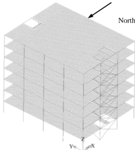
The Finite Element (FE) model of the building is created using the LUSAS FE Software [3]. The model of a concrete building is shown in Fig. 3. The flat floors are created using the 3D flat thin shell element (QSI4) with a mesh of 15 x 15 for each of the 12 panels. The columns and beams are created using eight 3D thick beam elements (BMS3). The bracing members are created using 3D bar elements (BRS2). The bottom ends of the columns are fixed to the foundation.
Fig. 3 gives an appropriate representation of the actual structure based on the available frequency measurements [9]. The natural frequencies of the building are measured every stages of the construction [1].
Table 1 shows the comparison between the natural frequency measurements and numerical results of the three first modes, which are called NS1 (the first North South direction), EW1 (the first East West direction) and R1 (the first rotation).
Fig. 3. The seven storeys Cardington concrete building model
As shown in the table, the natural frequencies from the numerical results are close to the measured natural fquencies. This means that the model is appropriate to re-present the actual building.
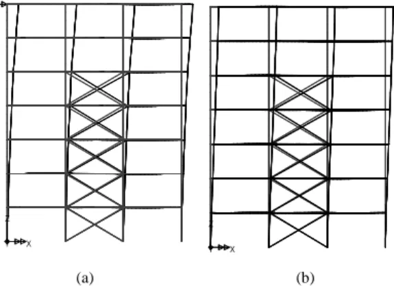
The 7th stage of the building model is used to inves-tigate the relationship between the static stiffness and the modal stiffness of the building. The modes in the North South (NS) direction are investigated, thus a point load is applied in the NS direction too. The static deformed shape and the first mode shape are shown in Fig. 4.
The floor mass of the building is a constant throughout the seven storeys and the masses of the columns are lumped in with the neighboring floors. Thus the modal mass of the i th mode of the building can be calculated by [7]:
∑
=
= 7
1 2
, ,
j i j j i
m M
M φ (28)
P=1
P=1
2 , ,
r cl r m
K
φ 2
1 , 1 ,
cl m
K φ 2
2 , 2 ,
cl m
K φ 2
3 , 3 ,
cl m
K φ KBsB
P=1P
L/2 L/2
TABLE 1.
COMPARISON BETWEEN THE NATURAL FREQUENCIES
Frecuency (Hz)
Stages NSI EWI RI
E N E N E N
1 2.90 2.733 3.14 2.828 3.42 3.25
2 1.77 1.902 1.86 1.885 2.14 2.33
3 1.36 1.245 1.36 1.343 1.61 1.75
4 1.04 1.062 1.04 1.159 1.28 1.44
5 0.87 0.889 0.87 0.933 1.06 1.18
6 0.71 0.735 0.73 0.769 0.87 0.99
7 0.60 0.619 0.61 0.648 0.76 0.83
E: experiment, N: numerical
TABLE 2.
RATIO OF THE MODAL DISPLACEMENTS TO THE STATIC DISPLACEMENT OF THE CONCRETE BUILDING
Modes Frequency (f) hz Modal Mass (mkg i) Modal Stiffness (kn/m mi) Mode Shape at the Critical Point (φcl,i)
Modal Disp. at the Critical Point due to each Mode*
Total Modal Displ.
Ratio, %
1 2 3 4 5 6 7 8
NS1 0.619 1.120E+06 1.697E+07 0.955 5.372E-08 5.372E-08 85.6
NS2 1.694 1.211E+06 1.372E+08 0.983 7.037E-09 6.076E-08 96.9
NS3 2.956 1.443E+06 4.979E+08 -0.759 1.158E-09 6.192E-08 98.7
NS4 4.208 1.116E+06 7.801E+08 -0.624 4.996E-10 6.241E-08 99.5
NS5 5.261 1.010E+06 1.104E+09 -0.319 9.200E-11 6.251E-08 99.6
NS6 6.446 1.217E+06 1.996E+09 -0.130 8.467E-12 6.252E-08 99.7
NS7 7.525 1.071E+06 2.394E+09 -0.027 3.096E-13 6.252E-08 99.7
Static displacement at the critical point, ui 6.273E-08 100.0
*The modal displacements at the critical point due to each mode are calculated by :
∑
== k
i mi i cl k cl
K u
1 2
, ,
φ
s k cl u u ,
i m
i cl
K , 2
,
(a) (b)
Fig.4. (a) Displaced shape; (b) The first mode shape (NS direction)
where φj,iis the normalized value of the j th floor in
the i th mode shape (provided by LUSAS results) and
Mj is the total masses of the j th floor and concerned
columns and bracing members. Once an eigenvalue analysis has been conducted, the modal stiffness of the associated mode can be calculated using equation (9).
The ratio of the modal displacements up to the k th mode to the static displacement of the concrete building are given in Table 2.The term of ‘mode shape at the critical points, φcl,i of the building in
column 5 of Table 2 are the normalized displacement of the i th mode at the NS direction. The ratio between the total modal displacement and the static stiffness can be drawn in Fig. 5.
Fig. 5. Ratio between the modal displacement to the static displacement
From Table 2 and Fig. 5, it can be seen that: 1. As the number of the mode considered increases
(the 1st mode to the 7th mode), the difference between the total modal displacement and the static displacement decreases as shown in the graph.
2. The first mode dominates the total modal displacement of the building, i.e., 85.6%, it means using the first mode of the modal stiffness is about 15% less than the static stiffness of the building. Using the first two modes usually is accurate to predict the structural responses of the buildings, i.e. about 97%.
3. Equation (16), which shows the relationship between the static stiffness and the modal stiffness, is verified for the seven storeys concrete building with the ratio is about 100% after the first 7 modes considered.
IV.CONCLUSIONS
The relationships (Equations (16) and (18)) between static stiffness and modal stiffness of a structure are derived on the basis of the definitions of the two stiffnesses. The relationship is applicable to any linear system.
The first mode of the modal stiffness of a structure is always larger than the static stiffness if the critical point and the maximum mode value are at the same node.
1. The verifications show that the first mode dominates the summation of the Equation (16). 2. The greater the number of modes being
considered, the smaller the difference between the total modal displacement and the static displacement of a structure.
REFERENCES
[1] A. J. Bougard and B. R. Ellis, 1998, “Vibrating testing of the
Cardington Framed Building”, Proceeding of the 3rd
Cardington Conference, Bedfordshire, UK.
[2] R. W. Clough and J. Penzien, 1993, Dynamics of Structures,
London, Mc. Graw-Hill. Inc.
[3] FEA Ltd, 2005, LUSAS User Manual,
Kingston-Upon-Thames, UK.
[4] Istruct E, 2002, ”The institution of structural engineers”. The
Use of Computers for Engineering Calculations. London.
[5] T. Ji and B. R. Ellis, 1997, “Effective bracing system for
temporary grandstands”. The Structural Engineer, Vol. 75, No. 6, pp. 95-100.
[6] T. Ji, 2003, “Concepts for designing stiffer structures”. The
Structural Engineer, Vol. 81, No. 21, pp. 36 - 42.
[7] Kim, 2001. "Effect of stiffness and mass variations on the
seismic response of reinforced concrete frames”. Journal of
Engineering and Applied Science, Vol. 48, No.5, pp. 919.
[8] H. Liu, Z. Yang, et al., 2005. "Structural identification and
finite element modeling of a 14-story office building using recorded data”. Engineering Structures, Vol. 27, No. 3, pp. 463-473.
[9] E. Wahyuni and T. Ji, 2004, ”The dynamic characteristics of a
concrete building from construction to completion”.
Proceedings of the 7th International Conference on Computational Structures Technology, 7-9 September 2004,
Lisbon, Portugal.
X Y Z
X Y Z
80 85 90 95 100 105