Efficient Clustering Protocol Based on Stochastic
Matrix & MCL and Data Routing for Mobile
Wireless Sensors Network
Omnia Mezghani
1, Pr. Mahmoud Abdellaoui
2- Senior Member IEEE
1
National Engineering School of Sfax (ENIS), Sfax University,Tunisia
2
National Engineering School of Electronics and Tel-Communication (ENETCOM), Sfax University, Tunisia
Abstract: In this paper, we have already presented a new approach for data routing dedicated to mobile Wireless Sensors Network (WSN) based on clustering. The proposed method is based on stochastic matrix and on the Markov Chain Cluster (MCL) algorithm to organize a large number of mobile sensors into clusters without defining the required clusters number in advance. It is based on mobile sensors connectivity to determine the optimal number of clusters and to form compact and well separated clusters. Our proposed approach is a distributed method using nodes locations, degrees and theirs residual energies during the cluster head election. Simulation results showed that the proposed approach reduced the loss packets rate by 80%, the energy consumption by 30% and improved the data delivery rate by 70% compared to LEACH-M protocol. Moreover, it outperforms the E-MBC protocol and reduced the average energy consumption and loss packets rate by 60%; as well as it improved the success packets delivery rate by 40%.
Keywords: Mobile WSN, clustering, stochastic matrix, localization, mobility, energy consumption.
1.
Introduction
Recent advances in the world of microelectronics and wireless technologies have allowed the emergence of small sensors characterized by a constrained processing capabilities, wireless communication capabilities and a limited energy resource. A WSN is a computing paradigm based on the collaborative efforts of a very large number of self-organizing sensors. Sensor nodes are densely deployed in a sensing field to collect data from their environment and communicate it to the base station (BS) [1]-[4]. Thus, WSNs are used in a variety of applications such as smart habitat, military, forest fire detection, underwater applications, animal tracking, health monitoring, patient monitoring, etc. WSNs can be deployed in hostile areas such as volcano which make difficult to replace sensors batteries [5]. So, extending the WSN lifetime is a trivial task. In the literature, many papers showed that the radio module in a sensor node is the component which consumes the most part of energy (about 94%)because it is responsible to ensure the communication between sensor nodes [6]. For that, an appropriate data routing protocol should be used to optimize the energy consumption.
Several research considers static networks while developing routing protocols. In such networks, nodes are fixed and do not change their locations after deployment. However, nowadays many applications such as the natural disaster prevention, complex environment supervision and medical supervision, etc, require the presence of mobile components in a WSN [1]. In fact, there are varieties of applications
including mobile sensor nodes that should operate in all autonomy, collaborate together and transmit their data to the BS [2], [7]. Mobile sensors networks are characterized by a frequent topology change making more challenges for researchers [8]-[10]. Some data routing protocols consider that each sensor node can communicate directly with the BS. This is not a suitable assumption because sensor nodes are constrained by a limited source energy. Other solutions propose a multi-hop data routing. Hierarchical routing protocols have been widely used for WSNs and have demonstrated an energy efficiency and scalability[8]-[15]. The Hierarchical protocols organize sensor nodes in the network dynamically into groups called clusters. For each cluster, a sensor with some criteria is elected as cluster head. Then, the cluster head collects data from other sensors in its cluster and aggregates it to reduce data transmission and to save energy [16]-[19].
Many existing approaches assume that the number of clusters is known in advance. Thus, it is not the real world scenario because they avoid the dynamic creation of clusters according to the sensors mobility. For that, we considered, in this paper, a more general scenario and assume that formed groups depend on mobile sensors connectivity and position to generate more compact clusters.
In this context, the work in this paper fits in the field of modeling and simulating multi-hop mobile WSN and revolves around three axes. Firstly, we addressed the problem of dimensioning the network and propose the stochastic method to model this network. Secondly, we considered the network partitioning and we proposed a clustering method by reference to the stochastic matrix using the MCL algorithm. Then, we addressed the issue of data routing in a mobile WSN. Finally, we evaluated the proposed approach performance and compare it to the Mobile Low Energy Adaptive Clustering Hierarchy protocol (LEACH-M) and the Enhanced Mobility Based Clustering protocol (E-MBC) into the OMNet++ simulator.
2.
Related Work
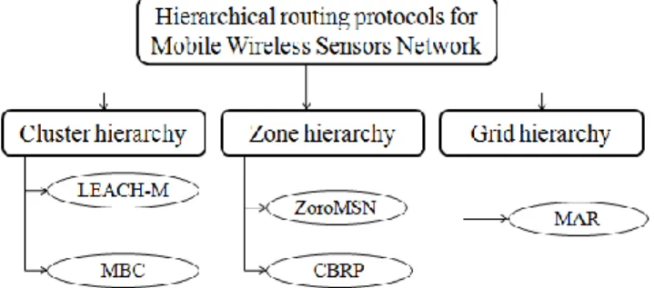
When the network size is larger, its management becomes difficult. Flat routing protocols work well with small size networks [20]. So, partitioning a large scale network is a key tool to save energy in each node in the network. One of the known structuring approaches is the hierarchy. The hierarchical technique is used to divide the network into subsets to facilitate network management especially routing process. As shown in Figure 1, we distinguish three types of node group: zone hierarchy, cluster hierarchy and grid hierarchy.
Figure 1. Hierarchical Routing Protocols for Mobile WSN
Cluster Hierarchy:In this type nodes group, a cluster is defined by a set of nodes and a head node named Cluster Head (CH). The CH is a gateway linking the cluster nodes to the base station directly or through other CHs. The CH is elected according to different criteria such: the energy level of a sensor, connection with other sensors, location, etc. The LEACH-Mobile is an extension of LEACH supporting the nodes mobility [21]. It outperforms LEACH in terms of loss packets rate in a mobile centric environment.
A node with low mobility is elected as CH. Once elected, the CH becomes stationary. Its election is based on the remaining energy, mobility and position given by the GPS system. It is based on data negotiation i.e. a mobile node transmits its data packet only if it receives a request from the CH. If it didn’t receive a request for 2 consecutive data frames, it should try to join a new CH [19], [21], [22].This protocol is dedicated for WSN with low-mobility because sensors have a low speed. It is not an adaptive mobility protocol where the packet loss rate increase when the speed or the number of sensors increase in a WSN.
The Enhanced Energy Efficient Clustering Algorithm (EEECA) [23] is based on non overlapping groups. Each cluster is managed by a cluster head which collects data packets from all the member nodes, aggregates and sends it toward the base station [23]. Although EEECA can minimize the energy dissipation and improve the mobile WSN lifetime, it has some drawbacks. It considers that all cluster heads are able to reach the sink whatever the distance. This assumption is unrealistic for large scale WSN and lead to a significant amount of energy consumption. Also, it assumes that each node know its position at each instant t.
The Mobility Adaptive Density Connected Clustering Algorithm (MADCCA) [24] is a density based clustering protocol. The clustering process is based on the exchange of the average relative velocity, the position and the density between neighborhood mobile entities. This proposed approach was targeted to vehicular traffic scenario [24]. This
protocol has two main drawbacks. Firstly, the vehicles move in the same direction. Secondly, they are equipped with GPS to be located.
The Mobility-Based Clustering protocol (MBC) [25] is designed for wireless sensors networks with mobile nodes. A node is elected as CH based on its remaining energy and mobility. The base station is fixed, the nodes are mobile and homogeneous. According to the number of sensors in a cluster, each CH creates a TDMA schedule. Each sensor node sends its data packets in its allocated time slot to its CH. When losing the connection with the corresponding CH, it broadcasts a request message to join a new CH. The main advantages of this protocol were energy efficiency, links stability and rate packet delivery success.
But, this protocol follows a proactive scheme and does not provide fault tolerance [19], [25]. An extension of MBC called Enhanced MBC (E-MBC) [26] has been proposed for mobile WSN. Similar to the MBC protocol, E-MBC is based on two phases: the set-up phase and the steady-state phase. In the first phase, mobile sensors are organized into clusters and a TDMA schedule is created. In the second phase, data packets are transmitted from sensors nodes toward the base station.
Each sensor node transmits its sensed data packet to the CH in its allocated time slot using a one-hop communication scheme.
Then, each CH aggregates the received data to transmit it toward the base station using a multi-hop scheme. If a sensor don’t has a data packet to transmit in its allocated time slot, it sends a special packet to indicate that it is still connected to the same CH. On the other side, a CH which has not receive any data packet in a time slot assumes that the corresponding sensor has left its cluster to another one. Thus, the CH eliminates the allocated time slot of the failed sensor node from the TDMA schedule.
The special packet has a small size compared to MBC allowing less energy consumption. Therefore, it informs CHs about its membership and about sensors nodes which are still alive. So, it is a fault tolerant and reliable clustering protocol [26].
Zone Hierarchy: In the second type nodes group, the network is divided into different zones. Zones construction relies on network information, thus requiring its instrumentation. These information can be static (such as sensors position in a fixed network) or dynamic (such as the energy level of sensor nodes). By shrinking the topology reorganization scope, the scalability can be increased. This is achieved as each zone performs distributive routing. Some protocols are able to create non overlapping zones while others are not. It reduces the reorganization complexity inferred by nodes movement [19].
The Zone-based Routing Protocol for Mobile Sensors Networks (ZoroMSN) [27] supports the mobility of sensors. It is a routing protocol that divides a mobile WSN into zones. This protocol is used to rotate data in a low-mobility network. In fact, it is applicable in a WSN using small area sizes and sensors with low speed [27].
where clusters are formed based on sensors mobility. Nodes are assumed to be homogeneous and know their locations. The base station is assumed to be stationary. The sensor field is divided into different zones.
Each zone has a unique identifier. The size of these zones determinates the neighboring of a sensor node. Each zone has a zone head which acts as a gateway between the sensors in the cluster and the base stations or with other zone heads. Routing is done by the zone head. The destination node collects several paths when receiving messages ”Route Request” (RREQ) from the source node and selects the most stable way to send their ”Route Reply” messages [28]. The Dynamic Clustering Mobile Data Collectors protocol (DCMDC) [29] is based on dividing sensors into groups called Service Zones (SZs). The localization of the mobility management traffic in a SZ reduces the communication overhead, bandwidth utilization and the roads establishment delay. This protocol is a self-organizing and adaptive dynamic clustering solution to keep MDC relay in the network. It reduces the energy consumption and prolongs the network lifetime [29]. However, it is characterized by an important handover interruption time , i.e., the delay from leaving one SZ and reaching a new one.
Grid Hierarchy: In the third type nodes group, nodes are arranged into a grid, which can be either calculated in a centralized manner by the BS and transmitted to all nodes, or performed by the sensors nodes themselves using a greedy algorithm. The main reason for constructing a grid structure is to reduce energy consumption by enabling the sensors located at grid points to acquire the forwarding information [30].
The Mobility Aware Routing (MAR) [31] is an hierarchical routing protocol based on localization. In this protocol a geographic grid is constructed in the sensing field and cluster heads are selected according to the sensors nodes mobility factor. The mobility factor refers to the number of sensors positions change. The objective of this CHs election is to select the node that has minimal mobility rate. Then, the node which has the lowest mobility rate is elected as CH during the CH selection process. This improves the CH connectivity with its associated nodes [31]. However, this protocol presented a major problem because it doesn’t consider the node energy in the CH selection process. Also, it doesn’t consider nodes location, which increases the data loss rate.
According to the literature survey, the existing works on clustering for mobile WSN are not optimal because they do not consider all constraints. Indeed, nodes mobility factor is not addressed appropriately and the majority of the existing classification systems are based on the adaptation of solutions dedicated for a fixed network to support nodes mobility. It is difficult and impractical to use these conventional schemes proposed for static WSN in a mobile WSN. Even if the node mobility is considered, the work is not addressed effectively to a dynamic network where nodes can migrate to different clusters. For this, mobile nodes movement must be properly addressed. In fact, the LEACH-M and Zoro-LEACH-MSN protocols are inappropriate for large-scale networks. The DCMDC is characterized by an important handover interruption time. The MAR does not consider nodes location and nodes energy in the CH selection process.
Therefore, sensors in MADCCA use GPS to be located. So, we have developed a new approach dedicated for a large mobile WSN that fills all the existing protocols limitations. This approach is based on the combination of three metrics at the CH election phase: the remaining energy, the degree and the position of each sensor. The proposed sensor location method is based on the combination of the GOMASHIO trapezoid method, ToA and RSSI techniques.
3.
Proposed Approach for Clustering
Partitioning a graph require to specify partitions size in advance. This is used with graphs that are homogeneous like for mesh or grid structures. But it avoids the creation of natural groups. Otherwise, this is not suitable for mobile networks in which sensors repartition is not planned in every region at every instant. In fact, mobile sensors nodes move freely in the sensing field.
In this setting, using Mobile Sensors Network needs a graph clustering that finds good partitions without specifying the groups member number in advance.
3.1 Graph Clustering Paradigm
Graph clustering considers that the formed clusters have the following properties:
A random walk in the graph G that visits a dense cluster will not leave this cluster until visiting many of its vertices.
Noting that a partition V is a collection of disjoint sets V1 ,.., Vd where each set Vi is a nonempty subset of V
and the union Ui=1..dVi is V .
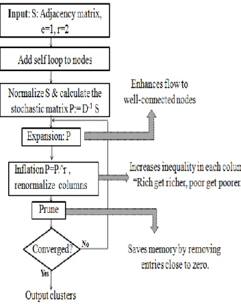
Emulating the network through a graph can be done by transforming it to a Markov graph. The Markov process stimulates random walk on a graph to find clusters. The idea is to use Markov to promote dense regions and downgrade the less favored regions (with less popular neighbors). This leads to clusters structure creation in the graph. The Markov process takes as input a stochastic matrix corresponding to the Markov graph; then it alternates the expansion and inflation which are both operators converting one stochastic matrix into another. Mathematically, the resulting process is called the Markov Chain Cluster process or MCL process [32]. 3.2 Classification by reference to a stochastic matrix
We proposed a classification method based on a stochastic matrix. The stochastic matrix reflects the affinity between the objects to be classified and is determined from the adjacency matrix which measure the similarity between them. The advantage of this method is its great flexibility due to the consideration of different resemblance measures (similarities measures, density measures, ...). The proposed classification approach is related to random walks on a graph by applying iteratively the stochastic matrix on this graph nodes [33].
3.2.1 Notations
S is an adjacency matrix having n variables that are measured on a set of N nodes.
is a stochastic matrix having N lines
and N columns . Each row of P is a probability vector (i.e.
). The ith line reflects the
communication link of the ith node with other nodes.
3.2.2 Stochastic Matrix Determination
The stochastic matrix P is determined from the similarity matrix S. with:
otherwise
neighbors
are
x
x
if
S
ij j i0
)
,
(
1
,
(1) To calculate P, we proceed with the normalization:
S D
P 1 (2)
where D is the diagonal matrix whose ith diagonal element is equal to the sum of the ith line of S:
n j i i jD
(, ); 1.. (3)An example of a graph (a set of nodes forming a network) which we apply on it the stochastic matrix for classification is discussed below.
3.2.3 Identifying classes from a stochastic matrix
We consider the graph G (V,w) where V is the set of vertices and w are the edges. The graph has N vertices corresponding to the different nodes. An edge is created from the vertex i to the vertex j if node i can communicate with node j ( i.e. the affinity between these node is not null). A random walk on this graph is a stochastic process that models a random movement from one node to another. It is defined by the stochastic matrix . This means that the probability of moving from node i to node j is given by the coefficient . Among the known properties of stochastic matrices, recalling that for a non negative integer n (n>0) the matrix
) gives the probability of moving from node i to node j in n hops. The node j is said accessible from i if there is a path from i to j i.e. if there is an integer n > 0 such that
. The nodes i and j communicate if there is a path from i to j and a path from j to i i.e. there are two integers n > 0 and m > 0 where
. The communication relationship is an equivalence relation. It defines equivalent classes of vertices, where each class is a set of maximum nodes that can communicate. Therefore, these classes correspond to the strongly connected components in the graph.
3.3 Markov Chain Clustering Process
In MCL, two processes are alternated repeatedly:
Expansion which is just normal matrix multiplication. It consists on putting the stochastic matrix P power n: the probability of a random walk from node i to node j in n steps.
Inflation which increase the weight of each vertices pair that have high entires and thus have a good chance to be belonged in the same cluster.
3.3.1 MCL Inflation
Given a matrix
, M≥0 and a non negative real r, the matrix resulting from rescaling each column in M with a power coefficient r is called ГrM. Гr is called the inflation operator with power coefficient r. Formally, the action of Гr :
is defined by [32], [34]:
k
i Miq r
r pq M pq M
r ) ( ) / 1( )
( (4)
3.3.2 MCL Algorithm Convergence
The algorithm converges always to a ”doubly idempotent” matrix i.e. every element in a column has the same value with other elements in this column (homogeneous column). In fact, a non-negative homogeneous column in a matrix M which is idempotent under matrix multiplication is called doubly idempotent [32], [34].
Definition 1. Let G = (V , w) be the associated graph of a non-negative idempotent matrix of dimension N, where
. The node
is called an attractor if
. If i is an attractor then the set of its neighbours is called an attractor system.
So, to interpret clusters, the attractors have at least one positive flow value within their corresponding row (in the steady state matrix ).
Each attractor is attracting the vertices which have positive values within its row. Then, the resulting sets form the clusters.
3.3.3 MCL Algorithm
Figure 2. MCL organigram
3.3.4 Running MCL Process
The graph presented in Figure 3 correspond to 7 connected mobile nodes in a sensing region. We applied the MCL algorithm on this graph to determinate the eventual groups forming this area.
Figure 3. Mobile sensor nodes graph
According the MCL algorithm, the first step consists to determinate the adjacency matrix S depending on the communication links between sensor nodes. Its resulting adjacency matrix is shown as:
0
1
1
0
0
0
0
1
0
1
0
0
0
0
1
1
0
0
0
1
0
0
0
0
0
1
1
1
0
0
0
1
0
1
1
0
0
1
1
1
0
1
0
0
0
1
1
1
0
S
Then, the parity dependence was removed by adding loops to each node in G. On the algebra side, adding loops corresponds with adding the identity matrix to S.
In the next step, we determined the diagonal matrix D as shown as:
7 (, ) 0 0 0 0 0 0 0 6 (, ) 0 0 0 0 0 0 0 5 (, ) 0 0 0 0 0 0 0 4 (, ) 0 0 0 0 0 0 0 3 (, ) 0 0 0 0 0 0 0 2 (, ) 0 0 0 0 0 0 0 1 (, )
i Si j i Si j i Si j i Si j i Si j i Si j i Si j
D
The stochastic matrix, obtained through the normalization based on Equation (2), is defined as following as:
77 ... 71 . . . . . . 17 16 ... 12 11 7 ) , ( 1 0 0 0 0 0 0 0 6 ) , ( 1 0 0 0 0 0 0 0 5 ) , ( 1 0 0 0 0 0 0 0 4 ) , ( 1 0 0 0 0 0 0 0 3 ) , ( 1 0 0 0 0 0 0 0 2(,)1 0 0 0 0 0 0 0 1 ) , ( 1 S S S S S S i j i S i j i S i j i S i j i S i j i S i Si j i
j i S
The calculation result of the preceding matrix (Adjacency matrix normalization) gives us the markov matrix P presented below: 33 . 0 33 . 0 33 . 0 00 . 0 00 . 0 00 . 0 00 . 0 33 . 0 33 . 0 33 . 0 00 . 0 00 . 0 00 . 0 00 . 0 25 . 0 25 . 0 25 . 0 00 . 0 00 . 0 25 . 0 00 . 0 00 . 0 00 . 0 00 . 0 25 . 0 25 . 0 25 . 0 25 . 0 00 . 0 00 . 0 00 . 0 25 . 0 25 . 0 25 . 0 25 . 0 00 . 0 00 . 0 20 . 0 20 . 0 20 . 0 20 . 0 20 . 0 00 . 0 00 . 0 00 . 0 25 . 0 25 . 0 25 . 0 25 . 0 P
Given the Markov matrix P, the value indicates the communication probability between the vertex j and the vertex i as compared to the other values in the jth column. A very important step is to iterate the alternation of expanding information flow via normal matrix multiplication and contracting information flow via applying .
The MCL process converges when every column in the matrix obtained after inflation presents the same value. The steady phase is reached as following as:
18
.
2
18
.
2
18
.
2
00
.
0
00
.
0
00
.
0
00
.
0
18
.
2
18
.
2
18
.
2
00
.
0
00
.
0
00
.
0
00
.
0
00
.
0
00
.
0
00
.
0
00
.
0
00
.
0
13
.
1
00
.
0
00
.
0
00
.
0
00
.
0
31
.
0
31
.
0
13
.
1
31
.
0
00
.
0
00
.
0
00
.
0
31
.
0
31
.
0
13
.
1
31
.
0
00
.
0
00
.
0
00
.
0
00
.
0
00
.
0
00
.
0
00
.
0
00
.
0
00
.
0
00
.
0
31
.
0
31
.
0
13
.
1
31
.
0
3
)
)
7
7
(
2
(
P
According to Definition1, the equivalence classes are
and
. The Figure 4 showed the resulting
clusters when using the MCL process.
Figure 4. Formed clusters by MCL algorithm
4.
Data Routing
In this section, we described our proposed approach to rotate collected data from mobile sensors nodes to the BS.
4.1 Process Network Model
We consider an heterogeneous network in which sensors nodes are randomly dispersed over the sensing field. We assumed that:
The sensors nodes are mobile and move randomly in the sensing field,
There are few anchors nodes knowing their positions in advance,
The sink is fixed,
All nodes have the same energy level initially and the same range which is equal to R.
Mobile nodes are located using the trapezoidal GOMASHIO approach combined with the ToA and RSSI techniques. The determined position is compared to each mobile node range; then, if it is lower than this range, it is admitted to be the final mobile node location.
4.2 Radio Energy Consumption Model
We implemented the same radio energy consumption model proposed in [35], [36], [37]. In this model, the consumed energy for transmitting k-bits message over a distance d is determined by
E
Tx(
k
,
d
)
(Equation (5)). The dissipated energy when receiving a k-bits message from a node at distance d is given byE
Rx(
k
)
(Equation (6)).d
k
E
k
E
d
k
E
Tx(
,
)
elec*
amp*
*
(5)
k
E
k
E
Rx(
)
elec*
(6)where and are the transmitting and receiving cost respectively, is the energy consumption when running the transmitter or receiver circuitry and is the energy dissipation for the amplifier transmissions. When launching the experiments in this paper, the radio energy consumption parameters are taken as:
E
elec
50
nJ
/
bit
,m
bit
pJ
E
amp
10
/
/
.4.3 Protocol Description
Our approach is based on three phases: the setup phase, cluster head election and data transmission.
4.3.1 Setup Phase
During the setup phase, anchors nodes forward an advertisement in order to collect data regarding the mobile nodes in their coverage. Mobile sensors nodes should determinate and send their locations, their residual energies and their degrees to the corresponding anchor node. Based on the received data, each anchor node calculates the stochastic matrix and launch the MCL algorithm to organize its member. More than one cluster can be found by an anchor node. During initialization, each anchor node broadcasts an announcement to start mobile nodes organization. After calculating the weight, a mobile sensor node selects the nearest anchor in its range and sends a message CH Announcement. Anchor node runs the MCL algorithm to organize the mobile sensors, to form the clusters and to elect for each cluster a CH having the higher weight.
4.3.2 Cluster Head Election
The anchor selects a group header for each group. This is a useful mechanism that reduces the complexity and increases the energy efficiency in a network [38]. During cluster head selection, anchor node calculates a weight for each mobile node in its coverage based on its residual energy, its proximity to this anchor and its degree. The weight is given by the following equation:
iai ri i e
d
e
W
deg
1
(7)
where
deg
i is the degree of the node i,e
ri is the residual energy and is the distance that separates node i to the anchor i in its range. This distance is determined using the combination of three methods: Gomashio based on trapezoidal method, ToA and RSSI. The corresponding process is given in Algorithm 1.Start location estimation;
if is_mobile_node then
broadcast an announcement to get anchors range
for j=1 to nb anchor do
Determine points coordinate resulting from different anchors range intersection dgij= position by the gomashio trapezoidal
drij= position by RSSI to anchor j
end
end
Gomashio error-correction;
if is_mobile_node then
position= Min(my_range,dgij ,drij ,dtij )
end
Algorithm 1: Mobile node position estimation
Cluster head should have the higher weight as compared to other nodes in the cluster. The cluster head election process is given in Algorithm 2.
Start Cluster Head Election;
if is_scheduled then
if this_is_anchor then
broadcast an organization announcement
end
end
Receive organization Announcement;
if is_mobile_node then
determine_distance_to_my_anchors();
if is_the nearest_anchor then
calculate my_degree();
send_CH_Announcement(myID,my_weight);
end
end
Receive_CH_Announcement;
Algorithm 2: Cluster Head election Algorithm CH election process is re-launched periodically. The main objective is to select a node as a cluster head that has higher neighbor nodes number, higher residual energy and is has the nearest position to the anchor node. Such CH selection serves two purposes:
1. Cluster head located near the anchor node provides better packet delivery and efficient energy consumption during communication with anchor node. When receiving data from other mobile sensors, the CH has to send its data packets to the anchor.
2. During communication between a CH and its member, such cluster head selection (with higher degree) can reduce the packets lost number because there is a possibility that CH and mobile nodes members are within transmission range of each other.
4.3.3 Data transmission
When generating a data, each mobile sensor node sends its data packet to its cluster head. The system assumes that if
any mobile node move away from a cluster to another, it loses the communication with the old CH and should try to join a new CH.
Each CH collects data from the surrounding nodes in its cluster, performs data aggregation and forwards it to the nearest anchor node in its range. Then, this anchor sends the data to the sink either directly or indirectly via some other anchors nodes.
5.
Performance Evaluation
An effective evaluation is important to convince users and to give them confidence regarding the proposed clustering methods.
5.1 Clustering Quality Evaluation
Different clustering algorithms are proposed and usually lead to different clusters in the sensing field. Even, for the different algorithms, the different parameters selection and data presentation may highly affect the final clustering groups. Our proposed method for clustering tends to : Optimize the number of clusters: by minimizing the number
of clusters and minimizing the number of isolated nodes and clusters with small size.
Maximize the formed clusters homogeneity: in terms of their cardinality.
Minimize the mean of the distances between the sensors within a cluster: minimize the intra-clusters inertia. Combine multiple criteria when electing the CH: Knowing
that the existing works have used only two criteria as well as the intra-clusters distance average was not taken into account.
Minimizing the intra-clusters distance (intra-clusters inertia) still an objective to obtain compact and well separated clusters. In fact, the intra-Clusters inertia measures the sensors concentration around the gravity center. More smaller is this inertia, little is the sensors dispersion around the gravity center. Lets recall that each cluster is characterized by a gravity center which is defined by µk in
the Equation (8):
K K
K K
C
i i
k C
i i
k
y
N
y
x
N
x
1
1
(8)
with: Nk = card(Ck). The intra-clusters inertia is defined in
Equation (9):
K
C
i i K
K
K
d
n
N
J
1
(
,
)
(9)
Where ni is node i. A good partition obtained by a clustering
clustering methods. The intra-clusters inertia average for a network is given in Equation (10):
K i C i K K KK w
K
J
n
d
N
J
1
(
,
)
(10) 5.2 Results
We evaluated the performance of our proposed clustering & routing protocol for mobile WSN through simulation results. Simulations are carried out in the OMNet++. It uses a modular structure to define the network architecture. It is based on INET framework which is well suited for simulations of WSNs as well as it supports nodes mobility [39]. The performance of our proposed protocol is compared to the routing protocols: LEACH-M and E-MBC [19], [21], [22], [27]. They were simulated for different number of nodes which are randomly distributed in a sensing field that have a dimension of 1000m × 1000m. Simulation parameters are shown in Table 1.
Table 1. Simulation Parameters
Parameters Values Field dimension 1000×1000 Initial energy in each node 1J
Nodes distribution Randomly deployed Number of nodes 25, 50,75,100 and 125
The considered metrics in the evaluations are energy consumption, number of clusters, Intra-clusters inertia, number of alive nodes, loss packets rate and data packets delivery percentage.
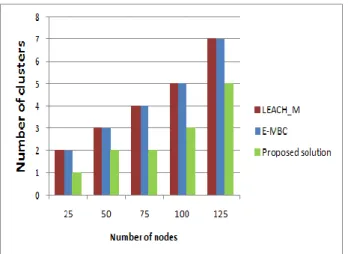
As shown in Figure 5, our proposed clustering method based on stochastic matrix and MCL algorithm reduced the number of clusters as compared to LEACH-M and E-MBC. In fact, LEACH-M and E-MBC are probabilistic algorithms which fix at advance the number of clusters and do not guarantee an adequate cluster-heads distribution in the network. But, the proposed approach uses a deterministic method to determine the appropriate number of clusters allowing compact and well separated partitions with an entire network coverage. This leads to a minimal number of isolated sensors and a minimal energy consumption.
When considering intra-clusters distances, as shown in Figure 6, our proposed approach succeed to form more compact clusters i.e. with low intra-clusters inertia. So, the proposed method showed a performance improvement compared to LEACH-M and E-MBC because the proposed clustering technique takes into account the sensors nodes proximity (sensors positions).
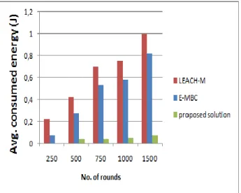
We simulated the average of the energy consumed by sensors nodes in the WSN, as shown in Figure 7, at node speed of 5 m/s. From Figure 7, we noted that LEACH-M did not provide efficient energy consumption. According to Figure 7 and since 1500 rounds, we noted that our approach minimized the energy consumption by 70% compared to LEACH-M and by 60% compared to E-MBC. This is due to: First, LEACH-M is a centralized protocol in which the BS is responsible of the clusters formation and the mobile sensors
nodes organization. But, in our approach anchor nodes organize and communicate the cluster ID for each sensor via shortest paths. Second, LEACH-M is based on data negotiation. Mobile nodes wait for a request (REQ Data) from the cluster head to send data in their allocated slot time in the TDMA schedule. If no response is obtained from the node, the CH will mark this member as mobile-suspect. Then, the CH repeats the same thing for the next slot time allocated for the same node. If no response, the sensor node is declared as mobile node and the slot time for that node is deleted from the TDMA schedule [40]. So, an extra traffic is added in the network. On the other hand, in our approach the mobile node which did not find a CH in its range stores its data in a buffer until the next round.
Figure 5. Generated clusters by the proposed approach, E-MBC & LEACH-M
Figure 6. intra-clusters inertia
Therefore, joining CHs in the E-MBC protocol is based on link stability (the longest connection time) rather than the minimum distance between sensors nodes and CHs. For thus, sensors may not join the nearest CH which leads to more energy consumption. But, the proposed protocol is based on the sensors degrees reflecting the number of neighbors as well as the minimum distance between sensors nodes and the anchors in the CH election phase. This leads to less power consumption.
Figure 7. Energy consumption average by the proposed approach, E-MBC & LEACH-M
As shown in Figure 8, the number of alive nodes is greater as compared to LEACH-M and E-MBC. After 500 rounds, this number was 40 by the LEACH-M protocol, 55 by E-MBC and 96 by the proposed protocol. After 1000 rounds, it decreased rapidly by LEACH-M and E-MBC until reaching respectively the value 20 and 32; whereas it reached 90 nodes by the proposed approach. In fact, as sensors nodes consume more energy by LEACH-M and E-MBC, the number of alive nodes decrease quickly.
So, in terms of network lifetime, our approach outperforms the both LEACH-M and E-MBC.
Figure 8. Alive nodes number by the proposed approach, E-MBC & LEACH-M
According to Figure 9 our proposed approach reduced the loss packets rate as compared to LEACH-M and E-MBC. In fact, When using 100 nodes, loss packets rate was 60% by the LEACH-M and 40% by the E-MBC protocol; whereas it was only 20% by the proposed approach. So, the obtained results proved that the proposed protocol outperforms the both protocols: LEACH-M and E-MBC.
As shown in Figure 10, the packet delivery ratio decreased when the number of nodes increased (for all protocols). But, data packets have more chance to achieve the BS by the proposed approach compared to LEACH-M and E-MBC. This increase achieved 70% compared to LEACH-M and
40% compared to E-MBC during the communication. This is due to the better CH election technique used in our proposed solution. Thus, LEACH-M and E-MBC sets the number of CHs in advance without identifying theirs degrees and theirs positions.
Figure 9. Loss packets number by the proposed approach, E-MBC & LEACH-M
This lead to misplaced CHs (i.e. overlapped CHs) or to disconnected nodes (i.e. long distances between CHs and members nodes). The proposed approach does not set the number of clusters in advance but determines the optimal number of clusters according to the mobility context and the nodes connectivity (an adaptive mobility protocol). It determines the optimal number of CHs depending on nodes positions, degrees and their residual energies to efficiently cover the network.
6.
Conclusion and Prospects
In this paper, we have already presented an efficient clustering protocol that determine the optimal number of clusters according to mobile sensors connectivities and positions. It allows to form compact and well separated clusters, to reduce the energy consumption and to ensure the best coverage in a mobile WSN. The proposed clustering algorithm is based on stochastic matrix & MCL. It is executed periodically at anchors nodes to organize sensors nodes into clusters and to elect new CHs using the combination of three parameters: nodes proximities to the anchor, nodes degrees and nodes residual energies. Firstly, we have discussed the existing clustering protocols dedicated to mobile Wireless Sensors Network. Then, we have detailed our approach based on stochastic matrix & MCL algorithm to efficiently organize mobile sensors nodes and to rotate data packets toward the base station.
The performance of our algorithm was compared to LEACH-M and E-LEACH-MBC protocols which fix in advance the number of clusters. Simulation results showed that the proposed protocol is more suitable for mobile WSNs. Among the improvements obtained by our protocol, we mentioned the reduction of energy consumption by 30% and the packets loss rate by 80%. On the other hand, we noted the increase of packets delivery rate by 70% compared to the LEACH-M protocol. On the other side, compared to the second competitor protocol ”E-MBC”, the simulation results showed a marked reduction concerning energy consumption and loss packets rate evaluated at 60% on the one hand; on the other hand, an increase in the delivery packets rate of 40%. Moreover, the proposed approach showed clearly its effectiveness when the network becomes dense-large scale with a high mobility rate.
Our future work tends to achieve more energy efficiency by implementing a MAC protocol.
7.
Acknowledgement
This work has been accomplished at WIMCS-Team research, ENETCOM; Sfax University. Part of this work has been supported by MESRSTIC Scientific Research Group-Tunisia
References
[1] O. Mezghani, M. Abdellaoui, "Improving Network Lifetime with Mobile LEACH Protocol for Wireless Sensors Network," 15th International conference on sciences and Techniques of Automatic control & computer engineering (STA'2014), Hammamet, Tunisia, December 21-23, 2014. [2] O. Mezghani, M. Abdellaoui, "Mobi-sim: A Simulation
Environment for Mobile Wireless Sensors Network," 3rd International Conference on Control, Decision and Information Technologies (CODIT'2016), Malte, April 6-8, 2016.
[3] M. Mezghani, R. Gatgout, G. Ellouze, A. Grati, I. Bouabidi, M. Abdellaoui, "Multitasks generic platform via WSN," International Journal of Distributed and Parallel Systems (IJDPS), Vol. 2, No. 4, pp. 54-67, 2011.
[4] D. M. Omar, A. M. Khedr, D. P. Agrawal, "Optimized Clustering Protocol for Balancing Energy in Wireless Sensor Networks," International Journal of Communication Networks and Information Security, Vol. 9, No. 3, pp. 367-375, 2017.
[5] A. Chakraborty, S. K. Mitra, M. K. Naskar, "A genetic algorithm inspired routing protocol for wireless sensor
networks," International Journal of Computational Intelligence Theory and practice, Vol. 6, No. 1, pp. 1-8, 2011. [6] G. Mathur, P. Desnoyers, P. Chuku, D. Ganesan, P. Shenoy,
"Ultra-low power data storage for sensor networks," Journal ACM Transactions on Sensor Networks (TOSN), Vol. 5, No. 4, pp. 96-101, 2009.
[7] M. Abdellaoui, Printed book (330 pages, 4 parts), "Multitasks-Generic-Intelligent-Efficiency-Secure WSNs and theirs Applications," LAMBERT Academic Publishing (LAP), ISBN: 978-3-330-04707-5, Part 2: "Intelligent Wireless Sensors Network," O. Mezghani, M. Abdellaoui, pp. 108-141, 2017.
[8] A. Shahzad, B .Sardar, "An Intelligent Routing protocol for VANETs in City Environments," 2nd International Conference on Computer, Control and Communication (IC4), Pakistan, Febrary 17-18, 2009.
[9] W. Heinzelman, A. Chandrakasan, H. Balakrishnan, "An Application-Specific Protocol Architecture for Wireless Microsensor Networks," Computer Journal of IEEE Transactions on Wireless Communications, Vol. 1, No. 4, pp. 660-670 , 2002.
[10]J. Yick, B. Mukherjee, D. Ghosal, "Wireless Sensor Network Survey," Journal of Computer Networks, Vol. 52, No. 12, pp. 2292-2330, 2008.
[11]K. Chan, H. PishroNik, F. Fekri, "Analysis of Hierarchical Algorithms for Wireless Sensor Network Routing Protocols," Wireless Communications and Networking Conference, IEEE, USA, March 13-17, 2005.
[12]X. Huang, H. Zhai, Y. Fang, "Lightweight Robust Routing in Mobile Wireless Sensor Networks," Military Communications Conference (MILCOM 2006), IEEE, Washington, October 23-25, 2006.
[13]Y. Miao, H. Jason, L. Renato, "Mobility Resistant Clustering in Multi-Hop Wireless Networks ," Journal of Networks, Vol. 1, No. 1, pp. 12-19, 2006.
[14]S. Madani, D. Weber, S. Mahlknecht, "A Hierarchical Position Based Routing Protocol for Data Centric Wireless Sensor Networks," 6th IEEE International Conference on Industrial Informatics (INDIN 2008), Korea, July 13-16, 2008.
[15]F. Tashtarian, A. Haghighat, M. Honary, H. Shokrzadeh, "A New Energy-Efficient Clustering Algorithm for Wireless Sensor Networks," 15th International Conference Soft COM on Software,Telecommunications and Computer Networks, Portsmouth, UK, September 27-29, 2007.
[16]S. Soro, W. B. Heinzelman, "Cluster head election techniques for coverage preservation in wireless sensor networks," Journal of Ad Hoc Networks, Vol. 7, No. 5, pp. 955-972, 2009.
[17]M. J. Handy, M. Haase, D. Timmermann, "Low energy clustering hierarchy with deterministic clusterhead selection," 4th International Workshop on Mobile and Wireless Communications Network (MWCN), Stockholm, Sweden, September 9-11, 2002.
[18]O. Younis, S. Fahmy, Distributed clustering in ad-hoc sensor networks: a hybrid, energy- efficient approach, Twenty-third Annual Joint Conference of the IEEE Computer and Communications Societies (INFOCOM’2004), Hong Kong, March 7-11, 2004.
[19]D. P. Shantala , B. P. Vijayakumar, "Clustering in Mobile Wireless Sensor Networks: A Review," International Journal of Advanced Networking & Applications (IJANA), Vol. 8, No. 1, pp. 134-136, 2016.
[20]S. Getsy, D. Sridharan. "Routing in mobile wireless sensor network: a survey," International Journal of Telecommunication Systems, Vol. 57, No. 1, pp. 51-79, 2014. [21]G. Renugadevi, M. G. Sumithra, " An Analysis on LEACH-Mobile Protocol for LEACH-Mobile Wireless Sensor Networks," International Journal of Computer Applications, Vol. 65, No. 21, pp. 38-42, 2013.
International Multi- Symposiums on Computer and Computational Sciences (IMSCCS'06), Hangzhou, China, June 20-24, 2006.
[23]K. J. Angel, E. G. Raj, "EEECA: Enhanced Energy Efficient Clustering Algorithm for Mobile Wireless Sensor Networks," World Congress on Computing and Communication Technologies (WCCCT), Tiruchirappalli, India, February 2-4, 2017.
[24]A. Ram, M. K. Mishra, "Mobility Adaptive Density Connected Clustering Approach in Vehicular Ad Hoc Networks," International Journal of Communication Networks and Information Security, Vol. 9, No. 2, pp. 222-229, 2017. [25]S. Deng, J. Li, L. Shen, " Mobility-based clustering protocol
for wireless sensor networks with mobile nodes," IET Wireless Sensor Systems, Vol. 1, No. 1, pp. 39-47, 2011. [26]L. Sahi, P. Khandnor, "Enhanced Mobility Based Clustering
Protocol for Wireless Sensor Networks," Proceeding of the International Conference on Electrical, Electronics, and Optimization Techniques (ICEEOT), India, pp. 687-692, March 3-5, 2016.
[27]N. Nasser, A. Al-Yatama, S. Kassem, "Zone based routing protocol with mobility consideration for wireless sensor networks," Journal of Telecommunication Systems, Vol. 52, No. 4, pp. 2541-2560, 2013.
[28]S. Awwad, C. Kyun, N. Noordin, " Cluster Based Routing Protocol for Mobile Nodes in Wireless Sensor Network," International Journal of Personal Communications, Vol. 61, No. 2, pp 251-281, 2011.
[29]A. Abuarqoub, M. Hammoudeh, B. Adebisi, S. Jabbar, A. Bounceur, H. Bashar, "Dynamic clustering and management of mobile wireless sensor networks," Journal of Computer Networks, Vol. 117, pp. 62-75, 2017.
[30]S. Verma, R. Kumar, P. Singh, " Survey on Grid Based Energy Efficient Routing Protocols in Wireless Sensor Networks," International Journal of Computer Applications, Vol. 101, No. 10, pp. 1-6, 2014.
[31]A. Shahzad, A. M. Sajjad , A. R. Khan, I. A. Khan, "Routing protocols for mobile sensor networks: a comparative study," International Journal of Computer Systems Science & Engineering, Vol. 29, No. 1, pp. 91-100, 2014.
[32]M. Hazewinkel, J. van Eijck, "Using MCL to extract clusters from networks, in Bacterial Molecular Networks: Methods and Protocols," Journal of Methods in Molecular Biology, Vol. 8, No. 4, pp. 281-295, 2012.
[33]S. Verdun, V. Cariou, E. M. Qannari, "Classification en référence à une matrice stochastique," 41th Statistic Days (JdS’2009), Bordeaux, France,May 25-29, 2009.
[34]L. Szilagyi, L. Medves,S. M. Szilagyi, "A modified Markov clustering approach to unsupervised classification of protein sequences," Journal of Neuro-computing, Vol. 73, No. 13, pp. 2332-2345, 2010.
[35]J. Kamimura, N. Wakamiya, M. Murata, "Energy-efficient clustering method for data gathering in sensor networks," 1st International conference on broadband networks (BROADNETS), San Jose, CA, USA, October 25-29, 2004. [36]S. Lindsey, C. S. Raghavendra, "PEGASIS power - efficient
gathering in sensor information systems," IEEE Aerospace Conference, Big Sky, MT, USA, March 9-16, 2002.
[37]O. Younis, S. Fahmy, "HEED: a hybrid, energy-efficient, distributed clustering approach for ad hoc sensor networks," Journal of IEEE Transactions on Mobile Computing, Vol. 3, No. 4, pp. 366-379, 2004.
[38]L. Buttyan, T. Holczer, "Private Cluster Head Election in Wireless Sensor Networks," IEEE 6th International Conference on Mobile Adhoc and Sensor Systems (MASS’09), TBD, Macau, China, October 12-15, 2009. [39]A. Varga, "The OMNeT++ Discrete Event Simulation
System," in the European Simulation Multiconference (ESM'2001), Prague, Czech Republic, June 6-9, 2001. [40]G. S. Kumar, V. Paul, K. P. Jacob, "Mobility Metric based
LEACH-Mobile Protocol," 16th International Conference on