A Distance-Based Data-Mule Scheduling Technique
for Lesser Nodal Delay in Wireless Sensor Network
Felomino P. Alba, Enrique D. Festijo and Ruji P. Medina
Graduate Programs, Technological Institute of the Philippines, Quezon City, Philippines
Abstract: Nodal delay in wireless sensor network is an indisputable factor in the medium of communication. Factor such as changeability of communication devices, network topologies, packet-sizes, and transmission rate demands to develop data-mule queue scheduling technique. Our proposed data-mule scheduling technique accomplish this through simulations using standard software written in C# by controlling data-mule schedules that collects data from all the nodes connected to the hop. The scheme identifies the hierarchical positions of static source nodes and the distance of mobile sourcenodes from the hop with rescheduling based on the newly acquired distances. Source nodes applied with data-mule scheduling technique resulted to lower nodal delay. Transmission of packet-data is efficiently and effectively improved.
Keywords: Data-mule scheduling, Wireless sensor network, Nodal delay, Queuing delay, Distance vector routing, Network layer.
1.
Introduction
In the recent year s, wireless sensor network (WSN) connects collection of interconnected receiving and transmitting devices across distances with system protocols. It is the future of communications by means of high speed packet-data exchanges. The changeability of devices, system, protocols packet-data size, transmission rate and topologies etc., are the fundamental driving force for the innovation in WSN. The controlled data-mule that collects packet-data from the source nodes reduced the nodal delay.
Several techniques have been developed to reduce nodal delays, including the use of low latency approximation that increases compression performance at lower computational cost and latency [1]. Scheduling and rescheduling in wireless sensor network are controlled by temporal spatial decision of network layers [2][3]. In extreme cases, nodal delays in packet transmission leads to general connection failures in wireless sensor networks[4]. Such latency stems from delays in either processing, queuing, transmission, or propagation [5] and may cause data delay, packet congestion, and higher response duration [6][7].
Among algorithms used in optimization, the genetic algorithm is the most prevalent tool used for optimization[8].In theory, the genetic approach should enable the orderly assignment of network tree nodes, thus leading to efficient scheduling. In practice, however, packet data transmissions by data-mules from source nodes to cluster heads of the network tree are not scheduled and this lack of scheduling in the routing process creates observed nodal delays.
Packet delay in data mule scheduling affects both static and mobile networks. In the first case, the problem occurs because the queues, which are based on the hierarchical position of source nodes in the network tree, are not being assigned schedules. For the second case, the problem occurs
because the queues, which are based on the distance of source nodes from hops, are not identified. This problem is further exacerbated when source nodes change position and their distance to hops also change, thereby requiring rescheduling. These problems are addressed in this study. To minimize nodal delay, an efficient scheduling technique for packet transmission is created. This allows the systematic queuing and transmission of data from all working source nodes to hops using a novel system of prioritization. The developed data-mule scheduler is tested in both static and mobile environments to ensure universal applicability.
2.
Related Work
Wireless sensor network is the most common way of data links communication, most of the network devices were supported by wireless sensor network [9][10]. Wireless sensor network is most widely used in communication systems that demand low cost, efficient and robust routing protocols including the transmission performance [11][12]. Created WCV wireless charging vehicle data-mule to jointly optimized dynamic multiple hop routing [13]
Data packet broadcast is the fundamental function of wireless sensor networks and provides an effective policy in all packet data protocol of connections and network topology[14]. While numerous study conducted on the performance of wireless sensor network has laid solid ground. The progress in the changeability of devices, network topologies, packet-sizes, and transmission rate are primarily impetus for the development of the DMS.
systematically using data-mule. Providing timely used of data-mule help lesser the nodal delay in wireless sensor network. DMS systematic queue schedules of data-mule for static source node and mobile source node, automatically reschedule the data-mule as its distance changes.DMS is designed to manage the priority schedules of the queues of data-mule. Improving the duration of wireless sensor network nodes lifetime for the coverage regions of interests with reduces optimal nodes [21]. Mobile technologies are relatively inflexible by limitations in link capacities, delivering real-time service difficult and erroneous [22].
3.
Proposed
Distance-based
Data-Mule
Scheduling Technique
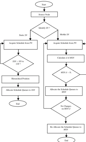
Our proposed system aims to minimize nodal delay in wireless sensor network. This is accomplished by using data-mule, which collects data from all the nodes connected to the network. Our system caters both static and dynamic source node. For clarity, we provide separate discussions for data-mule scheduling for static and mobile nodes, respectively (see section 3.1 and 3.2). To minimize the time required to collect data from each node, the data-mule is given a schedule based on distance to the source node. An illustration of how our scheme works is shown in Figure 1.
Figure 1. System Flowchart of Distance-based Data-Mule
Scheduling.
Table 1. List of Notations used
Notations Definitions
n Number of Source Nodes in the Cluster Head
SN Source Nodes
Nr Nearest to the Route
DN Destination Nodes of a working source nodes
d Distance of Source Node from the Route
NN Nearest Nodes
SSN Static Source Node
CH Cluster Head
MSN Mobile Source Node
dproc The time that node spends processing a packet. In this
paper it is assumed one (1) second.
dqueue The time that a packet spends in a queue at a node while
waiting for other packets to be transmitted. It is equal to transmission delay multiply by the average length of queue.
dtrans The time required to put an entire packet into the
communication media. It is computed by dividing the length of a packet in bits and transmission rate in bits per time unit.
dprop The time it takes a signal change to propagate through the
communication from a node to the next node. It is calculated by dividing distance from the node to the next node and the propagation speed of the media.
dnodal The time between the arrival of a packet at a node and its
arrival at the next node. It is the summation of dproc, dqueue, dtrans and dprop.
S Propagation speed mile/s
L Length of packet data being used for simulation
R Transmission speed from a – b
PN Processing Node
3.1 Data-mule scheduling for static source node
In our data-mule scheduling node, SSN A1, A2, & A3 n… acquires schedule from the PN. The source nodes that will be given the first data-mule schedule is the source nodes that is the nearest to the cluster head. The position of the source node is identified based on the hierarchical position of A1 in the network tree. The farthest node from the cluster head gets the last schedule from the PN in Figure 2.
Figure 2. Network Tree – Hierarchical Topology
Figure 2 presents the network tree of source nodes with neighbor’s nodes. Source nodes of A1, A2, A3, A4, A5, A6, A7,
A8, and A9 n… in the cluster head A are connecting source nodes given that the distance is equal to 0 creating a cycle from the PN. Source node A1is the parent node of cluster head A in the network tree source nodes relationship. The remaining sources nodes of the cluster head A are leaves of
n..
B1
B2
B3
B4
Cluster Head A Cluster Head B
A3
A4 A5
A6 A7 A8 A9 n…
A1
A2 Parent Node
Child Node
Leaves
Leave/s
Acquire Schedule from PN
Allocate the Schedule Queues to
MSN
Calculate d of MSN
MSN d = Nr
End
Acquire Schedule from PN
Start
Source Node
Static SN Mobile SN
Identify SN ?
Allocate Schedule Queues to SSN SSN = NN to
CH ?
Hierarchical Position
No Changes on MSN d
End
Re-Allocate the Schedule Queues to
the Network tree A. The number of source nodes in the series of cluster A is equal to the number of data-mule allocated by the PN. Process in the distribution of schedule is designed through the approach of who comes first is consider as parent nodes. The next connecting source nodes are considered as child nodes and will be given allocation after the cycle of the parent node has been completed. Moreover, cluster head B is a parent to child structure because; no leaves of child nodes are present. We always consider that cluster head in the network tree is represented by data-mule equal to the number of source nodes.
3.2 Data-mule scheduling for mobile source node
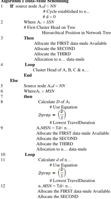
For MSN, schedule queues are allocated from the PN based on the distance of source nodes A1, A2, & A3 n…from the hop. The closest MSN to the hop gets the first schedule and listed as the priority of the queues. While the MSN changes its distance from the hop, the PN recalculates the d and allocates new schedule based on the newly acquired distance of connected MSN thus creating dynamic queues of MSN based on the changing distance of nodes from the hop. The algorithm then proceeds to the next cluster heads of B, C, & D n… Pseudocode of the procedure is depicted in Algorithm 1.
Algorithm 1 Data-Mule Scheduling
1 If source node A1d = NN
# Cycle established to n... # d = 0
2 Where A1 = SSN
# First Cluster Head on Tree
Hierarchical Position in Network Tree
3 Then
Allocate the FIRST data-mule Available Allocate the SECOND
Allocate the THIRD Allocation to n… data-mule
4 Loop
Cluster Head of A, B, C & n…
End Else
5 Source node A1d = NN
6 WhereA1 = MSN
7 then
8 Calculate D of A1
# Use Equation
# Lowest TravelDuration 9 A1MSN = Td< n…
Allocate the FIRST data-mule Available Allocate the SECOND
Allocate the THIRD Allocation to n… data-mule
10 Loop
11 Calculate d of n… # Use Equation
# Lowest TravelDuration 12 n..MSN = Td< n…
Allocate the FIRST data-mule Available Allocate the SECOND
Allocate the THIRD Allocation to n… data-mule
13 Loop
Cluster Head of A, B, C & n…
End
14 end if
4.
Results and Discussions
We have implemented all the simulations on this research through the use of a hierarchical position of SSN in the network tree and the distance of MSN from the hop, which would be comprised of CHA, B, C & n…Software written in C# was chosen as a simulator and the configurations used are shown in Table 2.
Simulations configurations include standard wireless mode specification of IEEE 802.11b, stop time equal to 1 second as constant value for processing nodes, distance of 100km, packet size of 128 kb the average packet-data weight of GSM (Global System for Mobile) which has the highest number of sources nodes, interval equal to 1 second, Interface queue of Droptail/PriQueue as mechanism of queuing and transmission data rate of 3 Mbps, which is the speed of wireless communication.
To evaluate the performance of Algorithm 1, multiple experiments were conducted on a different number of sources nodes from 10, 15, 25, 50, 100 and 250. All nodes have default size of 128kb.For each experiment; we have calculated the average results (see Fig. 8) consisting of the total average dnodal. QoS metrics such as network traffic prioritization rules NTPR, queuing and scheduling was obtained from the simulations to analyze the effectiveness and efficiency of our proposed algorithm.
Table 2. Simulation Configurations
Parameter/s Value/s
Wireless mode IEEE 802.11b
Stop Time (s) 1
Transmission range (km) 100 Packet Size (kb) 128
Interval (s) 1
Interface queue DropTail/PriQueue Transmission data rate (Mbps) 3
4.1 Nodal delay for static source node
To evaluate our proposed algorithm, we first perform a simulation to demonstrate the effect of having data-mule schedules for SNN given 10 SN, which are hierarchically positioned in the network tree in Figure 2.
Table 3. Nodal delay in milliseconds for SSN (SN=10)
SN dqueue dtrans dprop dnodal
A10 0.0084311 0.0000005 0.0084306 0.0168622 A4 0.0240931 0.0000005 0.0240386 0.0480782 A8 0.0395049 0.0000010 0.0395039 0.0790098 A1 0.0550903 0.0000015 0.0550888 0.1101806 A7 0.0706608 0.0000025 0.0706583 0.1413216 A5 0.0862411 0.0000030 0.0862381 0.1724822 A2 0.1017065 0.0000041 0.1017024 0.203413 A6 0.1173546 0.0000046 0.1173500 0.2347092 A9 0.1328979 0.0000051 0.1328929 0.2657958 A3 0.1484838 0.0000056 0.1484782 0.2969676
FIFO from A1, A2, A3, A4, A5, A6, A7, A8, A9A10.
Table 4. Decrease of DMS compared to FIFO
Queue DMS FIFO Disparity Decrease
1 0.0168622 0.1101806 0.0933184 9.33% 2 0.0480782 0.203413 0.1553348 15.53% 3 0.0790098 0.2969676 0.2179578 21.79%
Table 4 presents DMS first queue is = 0.0168622 (ms) vs 0.1101806 (ms) of FIFO is 9.33%, second = 0.0480782 (ms) vs 0.203413 (ms) of FIFO is 15.53% and third 0.0790098 (ms) vs 0.2969676 (ms) of FIFO is 21.79 % decrease compared to FIFO scheduled queues. The efficiency of DMS is illustrated better in terms of scheduling the SN.
Figure 3. Scheduled queues hierarchical tree
Figure 3 is the result of hierarchical position of SSN in the cluster tree. Queues schedule from the 10 SN where the priority is the parent A10 followed by the leaves of the succeeding tree nodes.
4.2 Nodal delay for mobile source node
To determine the performance of proposed algorithm in mobile source node, we conducted 10 iterations for 10 MSN
in an area of 10000km2. The iterations resulted in a 10
different priority queue schedules of source node based on the distance of nodes from the hop. The changes in distance of MSN automatically affect and create new queue schedules of all the nodes resulting to a newly acquired queuing schedule and a lower nodal delay value.
Table 5. Nodal delay in milliseconds for MSN (SN=10)
MSN dqueue dtrans dprop dnodal
A1 0.0781169 0.0000136 0.0781033 0.1562338 A2 0.1249854 0.0000205 0.1249649 0.2499708 A3 0.1093801 0.0000185 0.1093616 0.2187602 A4 0.0937461 0.0000156 0.0937305 0.1874922 A5 0.1405833 0.0000215 0.1405618 0.2811666 A6 0.0468605 0.0000097 0.0468508 0.093721 A7 0.0625029 0.0000122 0.0624907 0.1250058 A8 0.1562075 0.0000234 0.1561841 0.312415 A9 0.0312338 0.0000029 0.0312309 0.0624676 A10 0.0156075 0.0000009 0.0156066 0.031215
Table 5 presents the nodal delay of 10 MSN with different distances from the hop. In this scenario node 10 has the lowest dnodal because the distance of source node is 1321.9 km. The queue priority is depicted at table 6.
Table 6. MSN distances in 10 iterations
d1 d2 d3 d4 d5 d6 d7 d8 d9 d10
3121 2886 2528 2066 1849 1669 1630 1461 1403 2269
4998 4744 4349 3813 3545 3305 3249 2996 2897 4052
4566 4319 3938 3425 3172 2948 2896 2662 2572 3654
4020 3781 3415 3275 3239 3197 3191 3169 3174 3334
5149 5100 5050 5031 5043 5065 5072 5111 5080 5032
2362 2108 1716 1178 912. 675 620 376 286 1417
2727 2473 2077 1540 1272 1032 976 722 624 1780
5460 5313 5087 4791 4641 4522 4492 4364 4308 4916
1640 1441 1333 1438 1533 1669 1639 1752 1806 1389
1321 1465 1730 2097 2282 1448 2487 2664 2732 1932
Table 6 presents the different distances of 10 MSN. The simulation result shows that while the MSN moves across the area and changes its distance from the hop, the position of queue also changes creating systematic data-mule scheduling. The closer the MSN to the hop the highest priority queue it acquires from the PN in table 6. For example A10 first iterations resulted in1stqueue which is depicted in Table 7
with distance = 1321.9 from the hop, in the second iterations
A10is scheduled 2nd queue with changes its distance from 1321.9 to 1465, in the third iterations A10 is scheduled on the 3rdqueue as it changes the distance to 1730.7, in the fourth,
fifth, sixth and seventh iterationsA10 is scheduled on the 5th queue as changes its distance to 2097.2, 2282.1, 1448.2 and 2487.4, in the eighth and ninth iterations A10 is scheduled on 6th queue as changes its distance to 2664 and 2732.7 and on
the tenth iterations A10 is scheduled on 4th as changes its distance to 1932.6.
Table 7. MSN distances in 10 iterations
Queue Iterations
1 2 3 4 5 6 7 8 9 10
1 A10 A
9 A9 A6 A6 A6 A6 A6 A6 A9
2 A9 A10 A6 A9 A7 A7 A7 A7 A7 A6
3 A6 A6 A10 A7 A9 A9 A1 A1 A1 A7
4 A7 A7 A7 A1 A1 A1 A9 A9 A9 A10
5 A1 A1 A1 A10 A10 A10 A10 A3 A3 A1
6 A4 A4 A4 A4 A3 A3 A3 A10 A10 A4
7 A3 A3 A3 A3 A4 A4 A4 A2 A2 A3
8 A2 A2 A2 A2 A2 A2 A2 A4 A4 A2
9 A5 A5 A5 A8 A8 A8 A8 A8 A8 A8
10 A8 A8 A8 A5 A5 A5 A5 A5 A5 A5
A10
A4
A8
A1
A3
A7 A5 A2 A9 A6
Leaves
Parent Node
Figure 4. Comparison of 10 MSN iterations
Figure 4 presents the comparison of 10 MSN changes of distance from the hop for 10 iterations.
4.3 Nodal delay for varying number of source node
Rather than implementing a homogenous SN for the simulation, a heterogeneous SN scenario aimed to show NodaDelay of different SN values from 10, 15, 25, 50, 100 and 250 in table 8 while maintaining the transmission range of 10000km2 and transmission rate of 3Mbps.
Table 8. QueuingDelay, TransmissionDelay,
PropagationDelay andNodalDelay
SN dqueue dtrans dprop dnodal
10 0.0784410 0.0000028 0.0784381 0.1568820 15 0.1130017 0.0000030 0.1129996 0.2260034 25 0.1946371 0.0000070 0.1946300 0.3892742 50 0.3798615 0.0000165 0.3798449 0.7597230 100 0.7691648 0.0000365 0.7691283 1.5383296 250 1.9298121 0.0000655 1.9297465 3. 8596242
Figure 5. Nodal delay for different number of source nodes
Figure 5 presents incremental values of SN from 10, 15, 25, 50, 100 and 250. The simulation result indicates that the delay among number of sources is lesser having a systematic queue schedules of data-mule.
4.4 Comparison of DMS performance to some related works
Figure 6 presents SSN of 10 queues that are scheduled according to position in the hierarchical tree (see Figure. 3).By implementing Algorithm 1, the queue of 10 SN data-mule schedules which first to acquire schedule has the lowest nodal delay which is A10= 0.0084311 (ms)and the last to acquired schedule have the highest nodal delay which is A3 = .1484838 (ms).If applied using FIFO – First In – First Out, the A1 is the oldest nodes in the tree followed by A2, A3, A4,
A5, A6, A7, A8, A9A10 and n… Having queue schedule on 10
SN, the DMS proved efficiently creates systematic data-mule schedules.
Figure 6. Nodal delay comparison between FIFO and DMS
Figure 7. Duration comparison between FIFO and DMS
Figure 7 presents comparison of FIFO and DMS in terms of response duration from scheduled queues. DMS and FIFO both showed similar trends for queue schedules, though DMS was way better performing in scheduling. The DMS allocated queue schedule was clearly way ahead of the FIFO since the disparity for first queue is = 0.0933184, for the second is = 0.1553348 and for the third is = 0.2179578 which are all depicted in table 4. The disparity time between the FIFO and DMS could be used for another queue schedule of the following SN, showing the DMS systematic scheduling benefits the scheme in queues scheduling of communication network.
5.
Conclusions
nodes to processing node. Researches on source nodes approximation on arrival to processing nodes are topics greatly consider. Secondly, the simulation only identifies similar packet-size weight and transmission rate in mbps. It is a high time to conduct topic with multiple packet-sizes and different transmission rate with different network topology and multiple hops.
References
[1] J. Hou, L. P. Chau, N. Magnenat-Thalmann, and Y. He, “Low-latency compression of mocap data using learned spatial decorrelation transform,” Comput. Aided Geom. Des., vol. 43, pp. 211–225, 2016.
[2] L. Louail and V. Felea, “Latency optimization through routing-aware time scheduling protocols for wireless sensor networks,” Comput. Electr. Eng., vol. 56, pp. 418–440, 2016. [3] S. Malik, F. Huet, and D. Caromel, “Latency based group
discovery algorithm for network aware cloud scheduling,” Futur. Gener. Comput. Syst., vol. 31, no. 1, pp. 28–39, 2014. [4] J. Crowcroft, L. Levin, and M. Segal, “Using data mules for
sensor network data recovery,” Ad Hoc Networks, vol. 000, pp. 1–11, 2016.
[5] L. B. Lim, D. J. G. Spendlove, L. Guan, and X. G. Wang, “ADTH: Bounded nodal delay for better performance in wireless Ad-hoc networks,” Ad Hoc Networks, vol. 83, pp. 25– 40, 2019.
[6] M. Raj, N. Li, D. Liu, M. Wright, and S. K. Das, “Using data mules to preserve source location privacy in Wireless Sensor Networks,” vol. 11, pp. 244–260, 2014.
[7] K. Maraiya, K. Kant, and N. Gupta, “Wireless Sensor Network : A Review on Data Aggregation,” Int. J. Sci. Eng. Res., vol. 2, no. 4, pp. 1–6, 2011.
[8] V. P. Nambiar, M. Khalil-Hani, M. N. Marsono, and C. W. Sia, “Optimization of structure and system latency in evolvable block-based neural networks using genetic algorithm,” Neurocomputing, vol. 145, pp. 285–302, 2014.
[9] B. Neggazi, M. Haddad, and V. Turau, “A self-stabilizing algorithm for edge monitoring in wireless sensor networks,” Inf. Comput., vol. 1, pp. 1–10, 2016.
[10] D. T. Le, T. Le Duc, V. V. Zalyubovskiy, D. S. Kim, and H. Choo, “LABS: Latency aware broadcast scheduling in uncoordinated Duty-Cycled Wireless Sensor Networks,” J. Parallel Distrib. Comput., vol. 74, no. 11, pp. 3141–3152, 2014.
[11] A. Ajina and M. K. Nair, “Dynamic Network State Learning Model for Mobility Based WMSN Routing Protocol,” vol. 10, no. 2, pp. 266–278, 2018.
[12] D. Do, “Performance Analysis in Wireless Powered D2D- Aided Non-Orthogonal Multiple Access Networks,” vol. 10, no. 2, pp. 323–328, 2018.
[13] L. Shi, J. Han, D. Han, X. Ding, and Z. Wei, “The dynamic routing algorithm for renewable wireless sensor networks with wireless power transfer,” Comput. Networks, vol. 74, pp. 34– 52, 2014.
[14] J. A., K. R. S.V., and A. U. R., “Congestion avoidance algorithm using ARIMA(2,1,1) model-based RTT estimation and RSS in heterogeneous wired-wireless networks,” J. Netw. Comput. Appl., vol. 93, pp. 91–109, 2017.
[15] G. Carofiglio, L. Mekinda, and L. Muscariello, “Joint forwarding and caching with latency awareness in information-centric networking,” Comput. Networks, vol. 110, pp. 133– 153, 2016.
[16] T. Wang, S. Yao, Z. Xu, and S. Pan, “Dynamic replication to reduce access latency based on fuzzy logic system,” Comput. Electr. Eng., vol. 0, pp. 1–10, 2016.
[17] G. Citovsky, J. Gao, J. S. B. Mitchell, and J. Zeng, “Exact and Approximation Algorithms for Data Mule Scheduling in a
Sensor Network,” no. project 2010074, pp. 1–14.
[18] Y. Fan, H. Ding, L. Wang, and X. Yuan, “Green latency-aware data placement in data centers,” Comput. Networks, vol. 110, pp. 46–57, 2016.
[19] Q. Yang, “Latency-optimized high performance Data Vortex optical switching network,” Opt. Switch. Netw., vol. 18, no. P1, pp. 1–10, 2015.
[20] M. S. S. Khan, A. Kumar, B. Xie, and P. K. Sahoo, “Network Tomography Application in Mobile Ad-Hoc Network using Stitching Algorithm,” J. Netw. Comput. Appl., 2015.
[21] S. Biradar and M. Shastry, “Redundancy Elimination with Coverage Preserving Algorithm in Wireless Sensor Network,” vol. 10, no. 3, pp. 454–461, 2018.