doi: 10.7250/itms-2019-0002 https://itms-journals.rtu.lv
©2019 Ilya Jackson.
Simulation-Optimisation Approach to Stochastic
Inventory Control with Perishability
Ilya Jackson
Transport and Telecommunication Institute, Riga, Latvia
Abstract – In order to tailor inventory control to urgent needs of grocery retail, the discrete-event simulation model with realistic perishability mechanics is proposed in the paper. The model is stochastic and operates with multiple products under constrained total inventory capacity. Besides, the model under consideration is distinguished by quantity discount, uncertain replenishment lags and lost sales. The paper presents both mathematical description and algorithmic implementation. An optimisation framework based on a genetic algorithm is also proposed for deriving an optimal control policy. The proposed approach contributes to the field of industrial engineering by providing a simple and flexible way to compute nearly-optimal inventory control parameters.
Keywords – Genetic algorithm, perishability, simulation-optimisation, stochastic inventory control.
I.INTRODUCTION
In inventory control models, it is overwhelmingly assumed that products can be stored infinitely long [1]. Unfortunately, such an assumption does not correspond to reality because some products lose their valuable qualities over time, for instance, food, medicine and donor blood.
It should also be pointed out that the current success of online grocery retail has sparked interest in inventory control with perishability and encouraged researchers to study such models meticulously. Namely, according to the American Statistics Portal, in 2015 online grocery sales amounted to about $7 billion in the USA [2]. Moreover, these figures are expected to rise to $18 billion by 2020 and up to $26.87 billion by 2025 [3]. Thus, the future for online grocery retail is bright, and there is an urgent need for inventory control models that incorporate perishability mechanics.
II.RELATED WORK AND NOVELTY
The study on inventory control models with perishability dates back to Whitin [4]. In their seminal work the authors presented the model of production-inventory system with exponential deterioration rate and constant demand [5]. Later, Papachristos and Skouri developed an inventory control model with constant deterioration rate, time-dependent demand and partial backlogging [6]. Dye et al. extended this model and proposed a two-echelon inventory control model for deteriorating products [7].
Nowadays discrete-event simulation is the most dominant simulation paradigm for simulation-optimisation frameworks that, however, is not frequently used [8]. The first simulation-based optimisation of inventory control system dates back to Fu [9]. The model assumes zero replenishment lead time and
periodic review. The cost function comprises holding, purchasing, transportation and backlogging.
Among modern papers, metaheuristic in general and genetic algorithms in particular are distinguished. For instance, Peirleitner et al. considered a stochastic supply chain management problem [10]. The problem is stated as bi-objective optimisation problem. Overall supply chain costs are subject to minimisation, while the service level must be maximised. Such optimal control parameters as reorder points and lot sizes are derived by combining genetic algorithm with discrete-event simulation. In the same year, a discrete-rate simulation paradigm was used as a core to solve a single-product inventory control problem [11]. In this study, the model is developed in ExtendSim using an inbuilt genetic algorithm to find optimal control parameters. The recent research focuses on spare part inventory control for an industrial plant. Assuming that the demand is driven by maintenance requirements, spare part provision for a single-line conveyor-like system is considered [12]. Average cost per unit time is taken as the optimality criterion and optimisation is conducted using SimRunner’s inbuilt genetic algorithm.
Highlighting the novelty of the present research, it is important to point out that the considered simulation models a stochastic multi-product inventory control system that operates with deteriorating products, i.e., perishability mechanics is modelled in a way that closely corresponds to reality. These settings are characterised by explicit nonlinearity, which makes search space challenging to explore. The applied genetic algorithm is distinguished by integer chromosome encoding, uniform crossover and tournament selection.
III.METHODOLOGY
A. Inventory Control Model under Consideration
The model is developed to be implemented in the form of a discrete-event simulation.
The inventory control system stores a sequence of products 𝑃 = (𝑝1, 𝑝2, . . . , 𝑝𝑛)𝑛∈ℕ+ under limited total storage capacity
Imax. The model takes into consideration only such moments of
time, in which the system variables change. These discrete events are given as a sequence 𝑇 = (𝑡1, 𝑡2, . . . , 𝑡𝑛)𝑛∈ℕ+. Since the inventory control system works with perishable products, it is very convenient to represent the storage as a sequence of lots 𝑆𝑡𝑝= (𝑠1p,t, 𝑠2p,t, . . . , 𝑠𝑛p,t)𝑛∈ℕ+ replenished at different moments of time, such that for each 𝑆𝑡
𝑝
level is 𝐼𝑡 𝑝
= ∑ 𝑆𝑡 𝑝 𝑛
𝑖=1 . Days to expiration decrease during the simulation and the function ε(.) is introduced in order to model it in an iterative way:
𝐸
t+1 𝑝
= 𝜀(𝐸
t 𝑝
) = (𝑒0p,t− (𝑡
i+1− 𝑡i), . . . , 𝑒𝑛p,t− (𝑡i+1− 𝑡i)). (1) Empty and expired lots are removed, ∀𝑒𝑖p,t⩽ 0, 𝑆𝑡p← 𝑆𝑡p⁄𝑠𝑖p,t, 𝐸𝑡p ← 𝐸𝑡p⁄𝑒𝑖p,t and ∀𝑠𝑖p,t= 0, 𝑆𝑡p← 𝑆𝑡p⁄𝑠𝑖p,t, 𝐸𝑡p← 𝐸𝑡p⁄𝑒𝑖p,t (Fig. 1). Besides, the number of expired products is traced for later total expense calculation:
Expired
t 𝑝
= ∑𝑛 𝑠𝑖𝑝,𝑡[Φ].
𝑖=1 (2) where [Φ] is the Iverson bracket [13]:
[Φ] = {1 𝑖𝑓 𝑒𝑖 𝑝,𝑡
⩽ 0 .
else 0 (3)
Fig. 1. Mechanics behind perishability (modelling time is measured in days) [14].
Assuming that 𝑇𝑑𝑒𝑚𝑎𝑛𝑑𝑠𝑝 = (𝑡̂1, 𝑡̂2, … , 𝑡̂𝑛) includes only timings, when the new demand 𝑑𝑡𝑝 for a product p arises. Since the model under consideration is stochastic, demand size is a random variable D under a known distribution. In this regard, we introduce demand inter-arrival time as 𝑎𝑖= 𝑡̂𝑖− 𝑡̂𝑖−1, which is a value of a random variable A under a specified continuous distribution. Besides, a recursive function 𝑓𝑖=1(. ) is declared in order to fulfil arising demands depending on the available inventory capacity:
𝑓𝑖=1(𝑠 𝑖p,t, 𝑑t
𝑝
) = { 𝑠𝑖
p,t← 𝑠
𝑖p,t− 𝑑𝑡 p 𝑖𝑓 𝑠𝑖p,t≥ 𝑑𝑡p
else 𝑠𝑖p,t← 0, 𝑓i+1(𝑠
𝑖+1p,t , 𝑑𝑡p− 𝑠𝑖p,t)
, (4)
where i stands for an index of a lot to fulfil the demand. Fulfilled demand is also counted for later net profit calculation:
𝑆𝑎𝑙𝑒𝑠𝑡 𝑝
= {𝑑𝑡 p 𝑖𝑓 𝐼
𝑡p≥ 𝑑𝑡p
else 𝐼𝑡p . (5)
For each single product there is a pair of control parameters (𝑄𝑝, 𝑟𝑝) that determine the whole inventory control policy. According to the applied control rule, as soon as the current inventory level reaches the reorder point, namely 𝐼𝑡𝑝≤ 𝑟𝑝, the
inventory control system orders a new batch of size 𝑄𝑝. Besides, a Boolean status-variable 𝑠𝑡𝑎𝑡𝑝 ∈ {True, False} is declared in order to know if the batch is already ordered:
𝑜
t 𝑝
= {𝑄𝑝, 𝑠𝑡𝑎𝑡𝑝← True 𝑖𝑓 𝐼𝑡 𝑝
≤ 𝑟𝑝& 𝑠𝑡𝑎𝑡𝑝𝑖𝑠 False
else 0 . (6)
If an order is placed, the inventory-level will not be replenished instantly. Such a delivery lag is a random variable L under a known distribution. This means that the order 𝑜𝑡−𝑙𝑝 made at the moment of time ti ∈ T will be appended to the
storage 𝑆𝑡 𝑝
∪ 𝑜t-l𝑝, 𝐸𝑡 𝑝
∪ 𝑒𝑝 at the moment of time 𝑡𝑗 ∈ 𝑇 , such that 𝑡𝑗− 𝑡𝑖= 𝑙, where l is a value of a random variable L. For this reason, a supply function g(.) is introduced:
𝑔(𝑆𝑡𝑝, 𝐸
t 𝑝
, 𝑄𝑝) = { 𝑆𝑡 𝑝
, 𝐸𝑡𝑝 𝑖𝑓 𝑜𝑡+𝑙𝑝 = 0 else 𝑆𝑡𝑝∪ 𝑄𝑝, 𝐸
𝑡 𝑝
∪ 𝑒𝑝, 𝑠𝑡𝑎𝑡𝑝← False. (7)
It is important to point out that either a backorder-event 𝑑𝑡𝑝> 𝐼𝑡𝑝 or an overflow-event ∑𝑛 𝑆𝑡𝑝
𝑡=1 > 𝐼max can take place.
For this reason, the model traces backorders and overflows for later cost function calculation:
𝐵𝑎𝑐𝑘𝑜𝑟𝑑𝑒𝑟𝑠
t 𝑝
= {0 𝑖𝑓𝑑𝑡
𝑝
≤ 𝐼𝑡𝑝
else 𝑑𝑡𝑝− 𝐼𝑡𝑝 , (7)
𝑂𝑣𝑒𝑟𝑓𝑙𝑜𝑤
t 𝑝
= {0 𝑖𝑓 ∑ 𝑆𝑡
𝑝
≤ 𝐼max
𝑛 𝑡=1
else ∑𝑛 𝑆𝑡𝑝− 𝐼max
𝑡=1 .
(8)
The simulation executes functions in the following order: First, it checks expiration dates. Second, previously ordered goods are replenished. Third, the demand is fulfilled. Obeying this order of operations, the following equation to simulate inventory dynamics is derived:
(𝑆
t+1 𝑝
, 𝐸
t+1 𝑝
) = 𝑓 (𝑔(𝑆
t 𝑝
, 𝜀(𝐸
t 𝑝
), 𝑄𝑝)). (9)
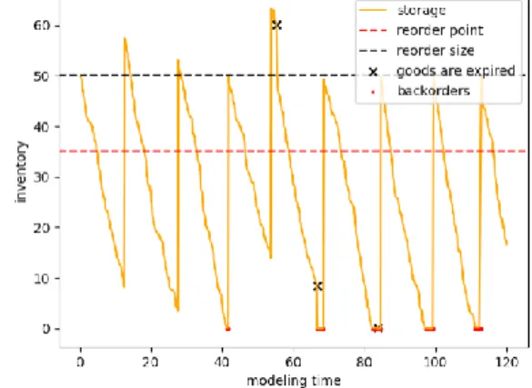
Figure 2 demonstrates inventory dynamics.
Fig. 2. Physical flow (modelling time is measured in days).
Ordering cost takes into consideration both purchase price and transportation cost. The model adopts the cut-off point quantity discount [15]:
𝑐𝑝(𝑄𝑝) = {
𝑐𝑝𝑓𝑜𝑟 0 < 𝑄𝑝≤ 𝛽 1
𝑘2𝑐𝑝𝑓𝑜𝑟 𝛽1< 𝑄𝑝≤ 𝛽2
𝑘𝑛𝑐𝑝𝑓𝑜𝑟 𝛽n-1< 𝑄𝑝≤ 𝛽𝑛
, (10)
where ordering costs for a physical unit 𝑐𝑝(𝑄𝑝) is a function of an order quantity, such that 𝐵𝑝= (𝛽
1 p
, 𝛽2p, . . . , 𝛽𝑛 p
) is a series of cut-off points and 𝐾𝑝= (1, 𝑘
2 𝑝
, . . . , 𝑘𝑛 𝑝
), ∀𝑘𝑖𝑝∈ [0,1]is a series of corresponding discount factors (Fig. 3).
Unit inventory cost ℎ𝑝 is constant and corresponds to inventory cost associated with the product p during demand inter-arrival lag. We also consider that every single out-of-stock (backorder) is associated with a loss of business reputation. Namely, if the demanded product is backordered, a customer is literally forced to search for a substitute. Every backordered unit is associated with a constant fee 𝑏𝑝.
Fig. 3. Cut-off point quantity discount (quantity is measured in pallets).
Overflows are also penalised by a constant fee 𝜔𝑝. In the real world, such expenses are associated with reverse logistics. Besides, when the lot is perished, penalty 𝜅𝑝related to recycling of expired goods arises. Based on the introduced variables, total costs associated with a product p can be calculated as follows:
𝑇𝐶𝑝= 𝑐𝑝∑𝑜 𝑡 𝑝
+ ℎ𝑝∑𝐼 𝑡 𝑝
𝛥𝑡 + 𝑏𝑝∑𝐵𝑎𝑐𝑘𝑜𝑟𝑑𝑒𝑟𝑠 𝑡
𝑝
+ 𝜔𝑝∑𝑂𝑣𝑒𝑟𝑓𝑙𝑜𝑤
𝑡 𝑝
+ 𝜅𝑝∑𝐸𝑥𝑝𝑖𝑟𝑒𝑑 𝑡 𝑝
. (11)
Considering the fact that each unit of product p is sold at a constant 𝑝𝑟𝑖𝑐𝑒𝑝, the total net profit can be calculated as follows:
𝑁𝑒𝑡𝑃𝑟𝑜𝑓𝑖𝑡 = ∑𝑛 𝑝𝑟𝑖𝑐𝑒𝑝∑𝑠𝑎𝑙𝑒𝑠𝑝
𝑝=1 − ∑𝑛𝑝=1𝑇𝐶𝑝. (12)
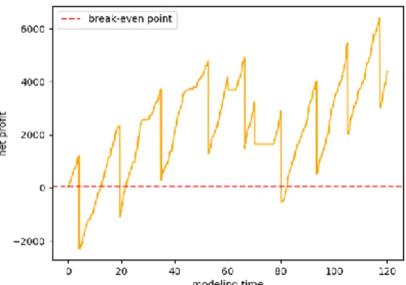
Figure 4 demonstrates the example of monetary dynamics.
It is worth noting that in the following examples total net profit is considered as the simulation output and subject to maximisation.
Fig. 4. Monetary dynamics (modelling time is measured in days).
B. Simulation-Based Optimisation
As it was demonstrated in the previous section, realistic stochastic inventory control problems could be naturally reformulated as discrete-event simulations. In simulation-optimisation based on a genetic algorithm, a simulation is utilised instead of an objective function in traditional form and a genetic algorithm is applied to find such simulation adjustments that would lead to the optimal output [16]. In general, methods of this kind are applied to solve stochastic optimisation problems of the following form:
𝑚𝑎𝑥
𝜃∈Φ𝐽(𝜃) = 𝐸[𝑌(𝜃)], (13) where θ corresponds to the vector of input parameters, and Φ stands for the set of feasible solutions. Y(θ) is the simulation output, such that the value of J(θ) is estimated based on the average of η replications [17]:
𝐽𝜂(𝜃) =1𝜂∑𝜂𝑖=1𝑌(𝜃). (14)
In the proposed simulation-optimisation approach, iterative search continues until specified search time is over.
C. Genetic Algorithm
Genetic algorithm is a metaheuristic search technique that mimics the “survival of the fittest” phenomena of natural selection. The algorithm was originally invented and deeply studied by Holland [18]. Applying a genetic algorithm to the inventory model under consideration, we are looking for such control parameters Q = (Q1, Q2, …, Qn) and r = (r1, r2, …, rn)
that result in the highest output (net profit). It is decided to use simple integer chromosome encoding, since it closely corresponds to the structure of the considered problem. Namely, the chromosome can be encoded as a list of integers 𝑣⃗= (Q1, r1,
…, Qn, rn), such that odd elements stand for order sizes and even
elements represent reorder points.
Fitness of an individual solution is the mean value of net profit calculated in several sequential replications (14) satisfying the following constraints:
If constraints are violated, fitness will take extremely low values due to infeasibility of such a solution.
Crossover operator is used to vary chromosomes from one generation to the next. The pivotal idea behind crossover is simple, namely, given two individual solutions that are both highly fit; however, for different reasons, crossover ideally results in a new solution that combines the features from parental [19]. In order to solve the considered problem, the uniform crossover is proposed (Fig. 5).
Fig. 5. Uniform crossover.
Uniform crossover is chosen for two main reasons. First, since genes in the individual solution correspond to different input variables, uniform crossover allows one to separate odd and even genes. Second, as it is mentioned by Michalewicz, uniform crossover significantly decreases chances of premature convergence [20]. In uniform crossover, individual genes in the chromosome are swapped with a fixed mixing ratio Probu,
according to the following algorithm:
Probu ← probability of swapping values
𝒗
⃗⃗⃗ ← first vector〈v1, v2, …, vn〉
𝒘
⃗⃗⃗⃗ ← second vector 〈w1, w2, …, wn〉 for i in range from 1 to len(vector) do
if Probu ≥ random number in range (0.0,
1.0)
swap the values of vi and wi return 𝒗⃗⃗⃗ and 𝒘⃗⃗⃗⃗
Besides, a genetic algorithm requires a mutation operator to perform the optimisation. Mutation can be treated as a background operator for assuring that the population is diverse enough to be efficiently exploited by crossover. The mutation operator can be expressed by the following algorithm:
Probm ← probability of replacing the value
𝒗
⃗⃗⃗ ← vector
for i in range from 1 to len(𝒗⃗⃗⃗) do
if Probm ≥ random number in range (0.0,
1.0)
𝒗𝒊 ← random integer in feasible range
return 𝒗⃗⃗⃗
The proposed optimisation framework takes advantage of tournament selection because it is a well-known robust approach for working with noisy fitness functions [21].
Tournament selection runs several “tournaments” among t_size individual solutions randomly driven from the population, such that the fittest individual in each tournament is picked for the following crossover. Algorithmically tournament selection can be implemented the following way:
Pop ← population
t ← tournament size, t_size ≥ 2
Best ← randomly picked from Pop
for i in range from 2 to t do
Next ← randomly picked from Pop
if Fitness(Next) > Fitness(Best)
Best ← Next
return Best
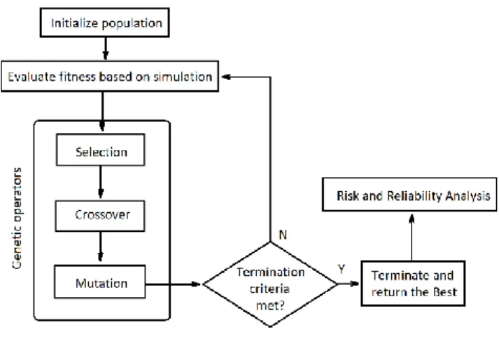
Moreover, it is worth mentioning that tournament selection works with parallel architectures and can be easily adjusted [19]. Figure 6 demonstrates the logic behind simulation-optimisation driven by a genetic algorithm.
Fig. 6. The logic behind simulation-optimisation.
IV.NUMERICAL EXPERIMENT
A. Defining the Number of Replications
In the considered problem, such input variables as D~N(μ, σ2), L~N(μ, σ2) and A~Exp(λ) are random; thus, the output (net profit) is also a random variable under some distribution. In this regard, it is important to decide, how many replications are sufficient. For this purpose, we use a method based on confidence intervals:
η = (𝑧α 2⁄
ζ 𝐶𝑉)
2
, (16)
where η is a minimum number of replications to achieve desired confidence interval width ζ for model with a coefficient of variation CV [22].
TABLE I
ANDERSON–DARLING NORMALITY TEST
Statistic Critical value Significance level
0.716 0.787 0.5
Using this approach, we test the null hypothesis that a sample is taken from a normally distributed population, i.e., if the calculated statistic is smaller than the critical value, the null hypothesis that the data is drawn from normal distribution can be accepted for the corresponding significance level [23].
Assuming the confidence level of 95 % and corresponding 𝑧α 2⁄ = 1.96, we calculate the coefficient of variation using sample mean and variance CV = 1512.8/9968.2 = 0.15. Therefore, it is decided to work with a confidence interval of length 498.4 (5 % of the mean) running each simulation 36 times to take the average output that corresponds to the average net profit obtained during the simulation runs.
B. Optimisation
In order to test the proposed optimisation framework, it is applied to the 10-product stochastic inventory control problem under consideration. It is important to mention that both the simulation model and the optimisation framework are implemented in Python 3.7 and are open-source [24].
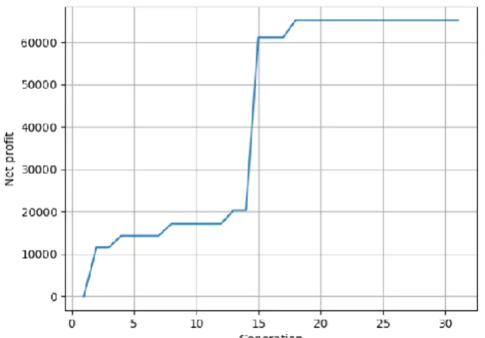
In the numerical example, a genetic algorithm uses the suggested hyper-parameters [19], namely, tournament size of 5, crossover probability of 0.35 and mutation probability of 0.05. The evolution lasts 31 generations, and each generation is populated with 100 candidate solutions. However, it is worth emphasising that hyper-parameter variation in the same range has not notably affected the convergence speed.
Fig. 7. The example of convergence path (net profit is measured in abstract monetary units).
The fittest candidate solution that results in the net profit of 6473 monetary units was obtained in 18 generations.
C. Risk and Reliability Analysis
The notable advantage of a simulation-driven approach is the possibility to conduct risk and reliability analysis (Fig. 8).
Fig. 8. Comparing the most promising solutions (net profit is measured in abstract monetary units).
Despite the fact that Solution 4 has the highest mean value, Solution 5 is distinguished by a smaller standard deviation; thus, it can be more attractive for a risk-averse decision maker. On the other hand, a risk-loving decision maker will be, most likely, interested in Solution 3, since it has the highest possible net profit.
V.CONCLUSION
To sum up, the proposed simulation-optimisation framework is both a simple and efficient approach to find nearly-optimal control parameters for a stochastic multi-product inventory control system that operates with perishable products. Besides, the key advantage of such an approach is the possibility to trace inventory dynamics in detail and involve the risk and reliability analysis in the decision-making process.
The study also concludes with a statement that integer chromosome encoding works properly in combination with uniform crossover and tournament selection. Moreover, fine tuning of hyper-parameters can provide a desirable balance between the convergence speed and the likelihood of premature convergence.
In future studies, it is expected to test this framework on problems with higher dimensionality and compare it to alternative metaheuristic techniques.
REFERENCES
[1] N. Khanlarzade, B. Yegane, I. Kamalabadi, and H. Farughi, “Inventory control with deteriorating items: A state-of-the-art literature review,” International Journal of Industrial Engineering Computations, vol. 5. No. 2, 2014, pp. 179–198. https://doi.org/10.5267/j.ijiec.2013.11.003
[2] The Statistics Portal, US consumers: online grocery shopping – statistics & facts, 2018 [Online]. Available: http://www.statista.com/topics/1915/ us-consumers-online-grocery-shopping/ [Accessed November 2019]. [3] Hexa Research, Report: Online grocery market expected to reach $26.9B
by 2025, 2018 [Online]. Available: https://www.grocerydive.com/news/report-online-grocery-market-expected-to-reach-269b-by-2025/543134/ [Accessed November 2019]. [4] T. Whitin, Theory of Inventory Management. Princeton, NJ: Princeton
University Press, 1957.
[5] R. P. Covert, and G. C. Philip, “An EOQ model for items with Weibull distribution deterioration,” AIIE Transactions, vol. 5, no. 4, pp. 323–328, 1973. https://doi.org/10.1080/05695557308974918
[7] C. Dye, “Deterministic inventory model for deteriorating items with capacity constraint and time-proportional backlogging rate,” European Journal of Operational Research, vol. 178, no. 3, 2007, pp. 789–807.
https://doi.org/10.1016/j.ejor.2006.02.024
[8] A. Gosavi, Simulation-based optimization 2nd ed. Berlin: Springer, 2015.
https://doi.org/10.1007/978-1-4899-7491-4
[9] M. Fu and D. Hill, “Optimization of discrete event systems via simultaneous perturbation stochastic approximation,” IIE Transactions, vol. 29, no. 3, 1997, pp. 233–243.
https://doi.org/10.1080/07408179708966330
[10] A. Peirleitner, K. Altendorfer and T. Felberbauer, “A simulation approach for multi-stage supply chain optimization to analyze real world transportation effects,” in 2016 Winter Simulation Conference (WSC), 2016, pp. 2272–2283. https://doi.org/10.1109/WSC.2016.7822268
[11] B. Zvirgzdina and J. Tolujew, “Experience in Optimization of Discrete Rate Models Using ExtendSim Optimizer,” in 9th International Doctoral Students Workshop on Logistics, Magdeburg, 2016, pp. 95–100. [12] F. Zahedi-Hosseini, “Modeling and simulation for the joint
maintenance-inventory optimization of production systems,” in Proceedings of the 2018 Winter Simulation Conference, 2018, pp. 3264–3274.
https://doi.org/10.1109/WSC.2018.8632283
[13] K. E. Iverson, “A programming language,” in Proceedings of the spring joint computer conferenceAIEE-IRE '62, May 1–3, 1962, pp. 345–351.
https://doi.org/10.1145/1460833.1460872
[14] I. Jackson, J. Tolujevs, S. Lang and Z. Kegenbekov, “Metamodelling of Inventory-Control Simulations Based on a Multilayer Perceptron,” Transport and Telecommunication Journal, vol. 20, no. 3, 2019, pp. 251–259. https://doi.org/10.2478/ttj-2019-0021
[15] E. Buffa and W. Taubert, Production-inventory systems planning and control, NTIS No. 658.4032 B8, 1972.
[16] D. Subramanian, J. Pekny, and V. Gintaras, “A simulation—optimization framework for addressing combinatorial and stochastic aspects of an R&D pipeline management problem,” Computers & Chemical Engineering, vol. 24, no. 2–7, 2000, pp. 1005–1011. https://doi.org/10.1016/S0098-1354(00)00535-4
[17] D. Koulouriotis, A. Xanthopoulos, and V. Tourassis, “Simulation optimisation of pull control policies for serial manufacturing lines and assembly manufacturing systems using genetic algorithms,” International Journal of Production Research, vol. 48, no. 10, 2010, pp. 2887–2912.
https://doi.org/10.1080/00207540802603759
[18] J. Holland, Adaptation in natural and artificial systems. Ann Arbor, MI: University of Michigan Press, 1975.
[19] T. Back, D. Fogel and Z. Michalewicz, Evolutionary computation 1: Basic algorithms and operators. CRC press, 2018.
[20] Z. Michalewicz, “Evolution strategies and other methods,” in Genetic Algorithms + Data Structures = Evolution Programs. Springer, Berlin, Heidelberg, 1996, pp. 159–177. https://doi.org/10.1007/978-3-662-03315-9_9
[21] B. Miller and D. Goldberg, “Genetic algorithms, tournament selection, and the effects of noise,” Complex systems, vol. 9, no. 3, 1995, pp. 193–212.
[22] M. Byrne, “How many times should a stochastic model be run? An approach based on confidence intervals,” in Proceedings of the 12th International conference on cognitive modeling, Ottawa, July, 2013. [23] N. Razali, and Y. Wah, “Power comparisons of shapiro-wilk,
kolmogorov-smirnov, lilliefors and anderson-darling tests,” Journal of statistical modeling and analytics, vol. 2, no. 1, 2011, pp. 21–33. [24] GitHub repository “metainventory” [Online]. Available:
https://github.com/Jackil1993/metainventory/tree/master/metamodels [Accessed November 2019].
Ilya Jackson is a PhD student of telematics and logistics at the Transport and Telecommunication Institute, Riga. He earned his Master’s degree in logistics from Kazakh-German University in 2016. He works as a Researcher and Lecturer at the Transport and Telecommunication Institute. His research interests include but are not limited to computational logistics, machine learning, evolutionary computing and production planning.