TECHNICAL UNIVERSITY OF CLUJ-NAPOCA
ACTA TECHNICA NAPOCENSIS
Series: Applied Mathematics, Mechanics, and Engineering Vol. 61, Issue Special, September, 2018
EVALUATION OF SUPPLY CHAIN COMPLEXITY AT MATERIAL FLOW
LEVEL FOR A ROMANIAN COMPANY
Camelia Ioana UCENIC, Claudiu Ioan RAŢIU
Abstract: The supply chains became more and more complex in last years. Each supply chain has different information and material flows. Complexity measure variation can be done at both information and material flow. This article presents an evaluation of material flow complexity dealing with the volume of production as variable, for the main product of a Romanian company from the point of view of sales (financial point of view). The actual level of production and the expected (scheduled) level of production are considered. Data collection took place in the weeks 3-17 from 2018 (January – April). The model uses the Shannon information entropy improved with Isik’s deviation of the outcome from the expected outcome value of the state. The usage of the model with outcome deviation is recommended because each state has its own complexity level. The complexity for a state with greater distance to the under control situation and the same frequency must be done first.
Key words: Complexity, Information entropy, Material flow, Outcome deviation, Supply chain
1. INTRODUCTION
The importance of supply chain increased in the last years due to globalization process. The management of supply chain became an essential issue for organizations as well as for the researchers. The involvement of suppliers and distributors has an important impact on the company competitiveness. The overall system turns out to be more complex. Nowadays, the overall complexity of the supply chain is a strategic issue. [1]
Each supply chain has different information and material flows. Complexity measure variation can be done at both information and material flow. The first step of its analysis is to define how complex is a supply chain. A set of quantitative indicators is required for it. The literature review mentions among the most used indicators the Shannon information entropy [2]. It defines complexity as a function of probabilities of different states. The entropy based measure was developed by many researchers.
The entropy can be measured at the level of different elements. This article presents an evaluation of material flow complexity dealing with the volume of production as variable.
2. SUPPLY CHAIN COMPLEXITY
“Complexity is defined as quantitative difference between predicted and actual states which are associated with the variety caused by the internal and external drivers in supply chain.” [3]
measures taken by the leading organizations. The study revealed that about 80% of the investigated firms consider they have a high complex supply chain and 60% recognize to have a high infrastructure cost basis. [4]
2.1 Factors which determine the supply chain complexity
There are external and internal factors which determine the supply chain complexity.
a. External factors
To meet the needs and requirements of the clients is a great challenge for each supply chain. Each company offers many products and services. This characteristic is ranked as the first or second reason for supply chain complexity. In addition, the customers want more choices about how and when are delivered their products. [5]
The globalization process is revealed as another main factor for supply chain complexity. The offer of the company must meet the specific requirements generated by the different cultures from different markets. The existence of international suppliers puts pressure on the supply chain.
b. Internal factors
The manner of the company organization can provide internal factors for increasing complexity. There are many option for technology selection and implementation. Each option determines a different level of complexity. Choosing an option which provides a lower level of complexity is not always possible because of cost or human resources constrains. The product life cycle brings also diverse levels of complexity. The features and the product attributes as well as its functions must be considered.
2.2 Trends in supply chain complexity
A company must rethink how its supply chain works in order to be cost efficient. Some of the most important trends are listed below.
Automation and robotics have a greater role especially in the western supply chains. To increase the automation level in manufacturing assumes a high investments costs. These costs are overcome in terms of company profitability.
A higher speed of innovation is another positive consequence of automation.
Digitalization of supply chains has an important impact on its complexity. Vast amount of information located in cloud provides a better understanding of market evolution. New ways of working can be developed at operational level and the supply chain become more responsive. [6]
The involvement of human resources is different in more complex supply chains. If in the past was more space for less skilled workers, nowadays are less job opportunities at this level. Now are required more educated workers and more competences at all business levels. The role of women in supply chain and in leadership is another worldwide trend in supply chain complexity. [7]
The degree of mobility penetration makes big changes in supply chain complexity. Many warehouses and transport operations use mobile devices. A growth in availability and variety off- the- shelf enterprise apps was noticed. [8]
3. DEFINING THE FLOWS AND THE TYPES OF SUPPLY CHAIN
COMPLEXITY
It is necessary to define the information and the material flows from a supply chain. This is the first step in order to explain the types of complexity. The literature review outlines many types of supply chain complexity. This article uses the: internal, external and total complexity.
3.1 Information and material flows
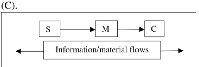
A simple supply chain is defined in three steps: supplier (S), manufacturer (M) and customer (C).
Figure 1: Scheme of a simple supply chain
The main tasks from a supply chain are the following:
Information flow
S M C
- A customer places an order to the manufacturer (M)
- This order represents the demand for the manufacturer
- The manufacturer (M) places an order to the supplier (S)
- This order represents the demand received by the supplier (S) from the manufacturer (M) Material flow
- The supplier(S) will supply to the manufacturer (M)
- This supply is the demand received from the supplier
- It will be supplied to the customer (C). - For the customer (C), it is the demand received from the manufacturer (M).
The information flow is given by the first four steps above mentioned, while the material flows is given by the last four steps.
3.2 Types of supply chain complexity
There are many approaches in the literature review for defining the supply chain complexity. One of the first attempts was done by Wilding who described the triangle of complexity: deterministic chaos, parallel interactions and amplifications. [9] Vachon and Classen introduced a four dimensional definition of complexity. [10] They make a connection between this four dimension complexity and the delivery performance. Other authors use the concept of complex adaptive system for the dynamic complexity. [11], [12]. Another approach is to classify the complexity in a supply chain as internal, external and total complexity. [13]
Internal complexity
The structure of a single business partner defines the internal complexity. It is generated by the material and information flows for the business partner of a supply chain. The variety of products, malfunction of machines, lack of raw materials and weak management are among the factors which directly affect the internal complexity.
External complexity
The material and information flows which are exported to a partner by another business partner gives the dimension of external
complexity. It is influenced by many factors as customer demand diversity, globalization, and level of innovation. A better cooperation between the partners of supply chain can help to reduce the external complexity at different levels.
Total complexity
The material and information flows within a business partner as well as amongst its other business partners define the total complexity. Total complexity covers internal and external complexity. [13]
4 METHODOLOGY
This article makes an evaluation of supply chain complexity using the entropy concept. Entropy based models can provide tools to quantify the supply chain complexity by delivering information required to describe the state of the system. [14]
4.1 Literature review
Entropy was used in many models. Entropy was introduced first in the thermodynamic systems. In the second stage, entropy was studied from the statistical point of view.
The classical entropy measure was implemented in the first models for complexity. [15], [16]. It was considered a good measure of flexibility. Shannon brings a great advance in this field because he proves its convenience in many area of technology and science. “Shannon’s entropy measures the average uncertainty associated with the prediction of outcomes in a random experiment.” [3]
First models presented a static measure of complexity. The newer models were improved by adding new data for a better description of the real system.
The experience obtained in industrial practice was also incorporated. This was an important fact because there are a limited number of complexity measures which can be implemented in the study of manufacturing systems.
information sharing by using computer simulation based on entropy is also presented.[18]
4.2 Evaluation of complexity with Shannon’s information entropy
The complexity measurement is done in order to have a scientific arithmetical scale which allows to compare the complexity values of an organization on various problems. The complexity of the supply chain is measured using the entropy. The starting point of the method is Shannon information entropy. It measures the average uncertainty in correlation with the prediction of outcome in a random experiment. The complexity is the variation between the actual and the expected flows. It is the same either for information flows or for material flows.
= − ∑ ∙ (1)
– Shannon’s information entropy of the discrete random variable
≥ 0Information is a positive quantity
0 ≤ ≤ 1,∑ = 1
The complexity from a supply chain has two types:
- Static or structural complexity: expected amount of information for defining the state of a system for a given period
- Dynamic or operational complexity: the expected amount of information for defining deviation from the schedule
= − ∑ ∑ ∙ (2)
- structural complexity - number of resources
– number of possible states for resource i – probability of resource I to be in state j
= − 1 − ∑ ∑ ∙ (3)
– operational complexity
– probability of the system to be in a “controlled scheduled state” ICS
1 − – probability of the system to be in an “out of controlled scheduled state” OCS
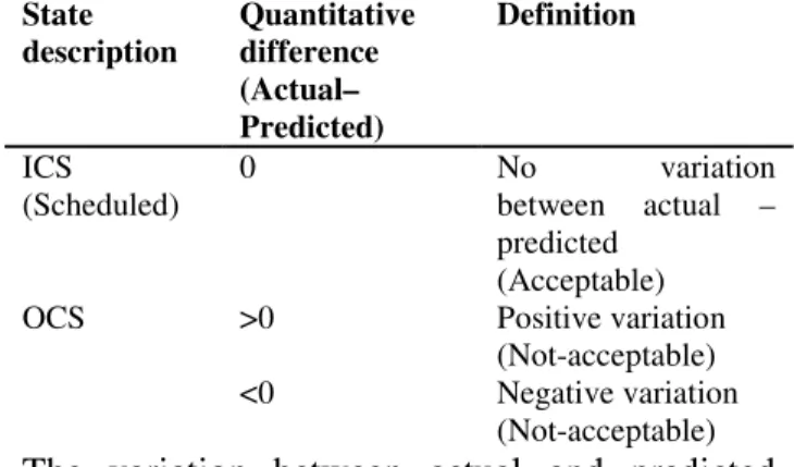
Table 1: Description of ICS and OCS – the state definition
State description
Quantitative difference (Actual– Predicted)
Definition
ICS (Scheduled)
0 No variation
between actual – predicted
(Acceptable) OCS >0 Positive variation
(Not-acceptable) <0 Negative variation
(Not-acceptable)
The variation between actual and predicted flows is consider representing complexity in this method. If the variation is 0 this means that no complexity occurs, but this happened only in ideal cases.
The deviation from the expected value describes the complexity for a particular state. The method proposed by Isik implements in the Shannon’s information entropy the deviation for each state. The formulas for the new entropy, modify structural complexity and modified operational complexity become as bellow:
= − ∑ (4)
= − ∑ ∑ (5)
= − 1 − ∑ ∑ (6)
It is considered the absolute value of, which represents the deviation of the outcome from the expected outcome value of the state.
5 CASE STUDY
This article presents a quantitative method in order to evaluate the complexity in a simple supply chain at the material flow level. The studied variable is the volume of production for the main product of the company from the point of view of sales (financial point of view). The actual level of production and the expected (scheduled) level of production are considered. The volume of production was chosen because of the frequent problems which occurred at the production level. A better management at this level will improve the quality at supply chain level.
as the name of its customers are not revealed due to confidentiality reasons.
A transformation coefficient was applied for all real data for the same reason. The application of the transformation coefficient was also useful in order to obtain smaller figures for simplifying the calculus. Data collection took place in the weeks 3-17 from 2018 (January – April).
The evolution of actual and scheduled production is illustrated in figure 1. Their difference is obvious, so one can say that is a complexity in this supply chain from the point of view of material flows.
Figure 2: Data evolution for actual and scheduled production values
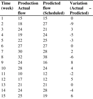
The next step of analysis undertakes the calculation for production variation, by subtracting from the actual flow the scheduled flow.
Table 1: Variation between actual and scheduled volume of production
Time (week)
Production Actual flow
Predicted flow (Scheduled)
Variation (Actual – Predicted)
1 15 15 0
2 18 27 -9
3 24 21 3
4 19 24 -5
5 22 25 -3
6 27 27 0
7 30 28 2
8 32 38 -6
9 24 16 8
10 28 24 4
11 10 12 -2
12 17 12 5
13 21 21 0
14 24 28 -4
15 25 19 6
The next step of the model consists of creating the probability distribution. The probability distribution was done according with the literature review.
It was used the same scale as in Isik researches because that models study the complexity of supply chain from the point of view of demand level variable. It is a direct relation between the demand level and the production level, so the same state intervals can be employed. They are listed in the following table.
Table 3: Categorization of the state [3] State interval State
description
Manageability Cost level
0 ICS - -
+6 ≤ ≤ 10 OCS1 Very difficult Cost1
+1 ≤ ≤ 5 OCS2 Manageable Cost2
−1 ≤ ≤ −5 OCS3 Manageable Cost3
−10 ≤ ≤ −6
OCS4 Very difficult Cost4
Each state interval has its own degree of manageability and an associate cost. The complexity is greater when it is a higher divergence of the expected value. The same situation occurs for the cost level.
The cost level 2 and 3 are lower than the cost levels 1 and 4. In control state ICS generates a very low cost or zero cost. No measures are required for this type of situation.
On the other hand, the other four situations require preventive and corrective measures in the supply chain. These situations have positive and negative variations from the out-of-control state which are not acceptable. The results of these actions are totally avoiding or decreasing the complexity from the supply chain from production point of view.
The next step is calculation of complexity values.
Table 4: Categorisation of the state State interval State
description
Frequency Probability
0 ICS 3 0.2
+6 ≤ ≤ 10
OCS1 2 0.13
+1 ≤ ≤ 5 OCS2 4 0.26
−1 ≤ ≤ −5
OCS3 5 0.33
−10 ≤ ≤ −6
OCS4 1 0.08
The next table provides the calculus of complexity. The structural complexity is calculated using formula (2) and operational
0 10 20 30 40
1 2 3 4 5 6 7 8 9 10 11 12 13 14 15 Actual - Scheduled Production
complexity is computed using formula (3). Probability of the system of being in control scheduled state is 0.2.
Table 5: Complexity calculations
State intervalProbability 0 0.2 0
+6 ≤ ≤ 10
0.13 0.382
+1 ≤ ≤ 5
0.26 0.505
−1 ≤ ≤ −5
0.33 0.527
−10 ≤ ≤ −6
0.08 0.291
Structural complexity
1.705
Operational complexity
1.364
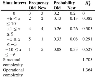
The next step of evaluation is to change between them the frequencies associated with OCS3 and OCS4 among them. So, the first three values remain the same but the previous frequency for the OCS3 become the new frequency for OCS4 and vice versa.
Using these new frequency, the model calculates the new values of probabilities. The changes appear just for OCS3 and OCS4.
Table 6: Categorization of the state with deviation State intervalFrequency
Old New
Probability Old New 0 3 3 0.2 0.2 0
+6 ≤ ≤ 10
2 2 0.13 0.13 0.382
+1 ≤ ≤ 5
4 4 0.26 0.26 0.505
−1 ≤ ≤ −5
5 1 0.33 0.08 0.291
−10 ≤ ≤ −6
1 5 0.08 0.33 0.527
Structural complexity
1.705
Operational complexity
1.364
In spite of changing the frequencies can be observe no change in the new values of the structural complexity. The real situation from the supply chain is different, so the value of structural complexity does not show the reality. The analysis of this shift demonstrates that the operational complexity of the whole system does not change in spite of the fact that the real situation is different.
These facts prove the necessity of implementing a more developed model for complexity analysis. There are different approaches in the literature review for describing the real situation. The Isik’s improved model was selecting for a better description of reality.
The model is carried out after the implementation of the deviation of the outcome from the expected outcome value for each state interval. Its absolute value is used |dij|.
The new structural and operational complexity is calculated with the formulas (5) and (6).
Table 7: Structural and operational complexity using the deviation of the outcome from the expected one
[X] State intervalFrequency
New
Probability New
0 3 0.2 0
+6 ≤ ≤ 10
2 0.13 7.063
+1 ≤ ≤ 5
4 0.26 1.515
−1 ≤ ≤ −5
1 0.08 1.583
−10 ≤ ≤ −6
5 0.33 2.331
New Structural complexity 12.492 Old structural complexity 1.705 New operational complexity
Old operational complexity
9.993 1.364
Figure 3: Comparison of complexity
The figure 3 presents a comparative analysis of the structural and the operational complexity measured in all three situations:
- initial situation,
- the situation with some frequencies changed - the situation with the consideration of the outcome deviation.
0 2 4 6 8 10 12 14
Structural complexity
Operational complexity
Comparison of complexity
As was previously presented, a shift in the frequencies does not bring any change neither for structural complexity nor for operational complexity. This fact is explained because the same probability values have the same complexity expressed through entropy.
The consideration of the outcome deviation will generate different values for the new structural and operational complexity. The new values are higher than the one without outcome deviation. This is true because each state has its own complexity level which must be considered. It is strongly recommended to evaluate the complexity at supply chain level at material flow using outcome deviation method in addition to the Shannon’s entropy model.
6 CONCLUSIONS
Complexity is correlated with a demand distortion in a supply chain, from the supplier to the manufacturer. Companies with a better control at supply chain level have competitive market advantages.
Last studies in the field shows the great potential of complexity management. The costs generated by product and process complexity in manufacturing counts up to 25% of the final expenditure.
It is a great need to integrate complexity management in the supply chain. Just a little number of firms are able to deal in a scientific manner with the complexity at their supply chain level. More attempts are empirical than scientific.
The classical entropy method shows if a supply chain system is in an under control or out-of-control state. Under out-of-control state occurs when the difference between the actual and expected (or scheduled) value is zero. The out of control state happens when this difference is not zero. The same probability values have the same complexity level, so the basic model which uses the classical complexity definition does not illustrate the real situation from the supply chain. It is necessary to have a method which helps us to map the degree of being out-of-control.
The implementation of outcome deviation from the expected outcome value provides better
results with respect to complexity costs generating by manufacturing for this study. The costs for the out-of-control states 1 and 4 are higher than the costs of OCS2 and OCS3. There are required countermeasures in order to decrease the complexity for these intervals. Corrective measures have to be implemented by the managers in the first stage. The following step is to design preventive measures. Complexity management is mandatory for each supply system.
If it is supposed that the system has two states with the same frequency values but with different distance from the out-of-control state one must reduce first the complexity for the state with a greater distance to the under control situation.
Further research must be done at all levels of supply chain instead of the empiric work. New complexity measures and improved models have to be developed and applied in manufacturing. Systems with higher complexity should be considered and improved in comparison with the systems with lower complexity.
The study was the first attempt for this company to evaluate in a scientific way the complexity generated in its supply chain by the production issues.
The Shannon’s entropy method was applied first. In the second stage, the model was improved with the implementation of outcome deviation proposed by Isik due to performance considerations.
Further work must be done for the other products from A category, according with ABC classification. A comparison of results will help the managers to rank the complexity problems and to propose measures for accepting, controlling, reducing and avoiding complexity.
7 REFERENCES
1. Perona, M., Miragliotta, G., Complexity Management and supply chain performance assessment: a field study and a conceptual framework, International Journal of Production Economics, Vol. 90, No.1, pp. 103 -115, (2004). 2. Shannon, C.E., The mathematical theory of communication, The Bell System Technical Journal, 27, pp. 379-423, (1948)
supply chain complexity, in Supply Chain Management, Edited by Penzhong Li, ISBN 978-953-307-184-8, (2011).
4. *** - PRTM, PwC, (2006)
5. Yami, Z., Tefen Management Consulting, Supply Chain Complexity – Dealing with A Dynamic System, (2016)
6. Schuh, L., Supply chain and logistics trends in 2017, National Logistics Association – Germany, (2017)
7. Sandberg, L., Managing Trends and complexity in supply chain, Manucore, (2017)
8. O’Byrne, R., 7 Supply chain and logistics trends to watch in 2018, Logistics Bureau, (2018) 9. Wilding, R., The supply chain complexity
triangle, International journal of physical distribution and logistic management, Vol. 28, No.8, pp. 599-616, (1998)
10. Vachon, S., Klassen, R., An exploratory investigation on the effects of supply chain complexity on delivery performance, IEE Transactions on Engineering Management, Vol. 49, No. 3, pp. 218-230, (2002)
11. Choi, T.I., et all, Supply networks and complex adaptive systems, Journal of Operational Management, Vol. 19, No. 3, pp 351-366, (2001)
12. Vollman, T., et all, Manufacturing Planning and control for supply chain management, 5th edition, Mc-Graw-Hill, New York, USA, (2005) 13. Isik, F., An entropy based approach for measuring complexity in supply chain, International Journal of production research, Vol. 48, No. 12, pp. 3681-3696, (2010)
14. Chen, Y. C., et all, An analysis of the structural complexity of supply chain networks, Applied Matematical Moddeling, Vol. 38, No. 9-10, pp. 2328-2344, (2014)
15. Calinescu, A., - Complexity in manufacturing: an information theoretic approach, Conference on complexity and complex systems in industry, pp. 30-44, (2000)
16. Sivadasan, S., et all, Advanced on measuring the operational complexity of supplier-customer systems, European journal of operational research, Vol. 171, No. 1, pp. 208-226, (2006) 17. Makui, A., Aryanezhad M. B., A new method
for measuring the static complexity in manufacturing, Journal of operational research, Vol. 55, No.5, pp. 555-557, (2003)
18. Martinez O.V., Entropy as an assessment tool for supply chain information sharing, European journal of operational research, Vol. 185, No. 1, pp. 405-417, (2008)
Evaluarea complexitatii lanțului de aproviziovare la nivelul fluxului de material pentru o companie românească
Rezumat: Lanțurile de aprovizionare au devenit din ce în ce mai complexe în ultimii ani. Fiecare lanț de aprovizionare are diferite informații și fluxuri de materiale. Variația măsurătorilor de
complexitate se poate realiza atât în ceea ce privește informațiile, cât și fluxul de materiale. Acest articol prezintă o evaluare a complexității fluxului de materiale, care se referă la volumul producției
ca variabilă, pentru produsul principal al unei companii românești din punct de vedere al vânzărilor
(punct de vedere financiar). Sunt luate în considerare nivelul real de producție și nivelul așteptat (programat) de producție. Colectarea datelor a avut loc în săptămânile 3-17 din 2018 (ianuarie -
aprilie).
Modelul utilizează entropia informației Shannon îmbunătățită cu abaterea lui Isik a rezultatului din
valoarea așteptată a rezultatului statului. Utilizarea modelului cu devierea rezultatului este
recomandată deoarece fiecare stat are propriul său nivel de complexitate. Complexitatea unei stări
cu o distanță mai mare față de situația sub control și aceeași frecvență trebuie făcută mai întâi.
Camelia Ioana UCENIC, Department of Management and Economic Engineering, Technical University of Cluj Napoca, 28 Memorandumului Street, Cluj Napoca, Romania, [email protected]