A coherent structure approach for parameter estimation in
Lagrangian Data Assimilation
John Maclean∗1, Naratip Santitissadeekorn2, and Christopher KRT Jones3
1,3Department of Mathematics and RENCI, University of North Carolina at Chapel Hill
2Department of Mathematics, University of Surrey, Guildford
June 16, 2017
Abstract
We introduce a data assimilation method to estimate model parameters with observations of passive tracers by directly assimilating Lagrangian Coherent Structures. Our approach differs from the usual Lagrangian Data Assimilation approach, where parameters are estimated based on tracer trajectories. We employ the Approximate Bayesian Computation (ABC) framework to avoid computing the likelihood function of the coherent structure, which is usually unavailable. We solve the ABC by a Sequential Monte Carlo (SMC) method, and use Principal Component Analysis (PCA) to identify the coherent patterns from tracer trajectory data. Our new method shows remarkably improved results compared to the bootstrap particle filter when the physical model exhibits chaotic advection.
1
Introduction
The problem of assimilating the path travelled by ocean instruments such as drifters to estimate states and/or parameters of dynamical systems is commonly known as Lagrangian data assimilation (LaDA). Every method for LaDA depends on the knowledge of error statistics for the observed
position of the drifter paths; typically, it assumes the normal likelihood function and uncorrelated errors of observed position among all drifters. In this paper, we explore a novel idea for LaDA that assimilates a “coherent (or persistent) structure” hidden in the Lagrangian path of the drifters
instead of directly using the observed positions. We discuss the main advantage of this idea in the situation where the number of drifters is large, observed position has small variance and the
flow is chaotic. We also demonstrate the improved accuracy of the parameter estimates of the new method when comparing with the particle filtering (PF) approach, which is apparent if the drifter paths are dominated by chaotic advection.
Modern satellite-tracked ocean drifters [7,13] have been recognized as an important source of data for oceanographic and climate research. Drifters travel near the surface and measure physical data such as surface temperature along their paths via drifter sensors [12]. In addition, they offer Lagrangian path data through the Doppler frequency shift on their satellite-based transmission.
∗
corresponding author, available [email protected]
The accuracy of drifter locations can be less than 150 meters [7], and there is a global ocean drifter set providing measurement data at a mean time interval of 1.2 hours spanning over a decade [13].
Oceanographic flows exhibit patterns at scales from metres to kilometres, and correspondingly
drifters are seen to move in eddies or gyres and follow currents, creating small and large-scale patterns which can be used to infer the sea-surface flows [14, 38]. These patterns are associated with fundamental structures of the flow, including stable and unstable directions, centres and
saddles. The goal of the current work is to infer the underlying flow state, or the parameter set governing the flow, from the patterns rather than directly from the drifter trajectories.
Several LaDA methods have been presented in the last decade for sequentially assimilating La-grangian path data into dynamical system models of the ocean [2, 25, 27, 29, 31, 40, 43, 44, 49]. These methods append a Lagrangian model of the drifter locations to the Eulerian flow model in
order to make inferences about how drifter locations correlate with model states; this approach also avoids the difficulty in which Lagrangian path data does not correspond to the fixed Eulerian grid
locations. The key challenge of Lagrangian Data Assimilation (LaDA) is that the Lagrangian path of the passive tracers or drifters can be strongly nonlinear, which makes it difficult to sequentially estimate model state variables or parameters by computationally efficient methods such as the
En-semble Kalman filter (EnKF) [2]. It has been emphasized in several pieces of work that a nonlinear, Bayesian filtering framework such as the Particle Filter (PF) is more reliable in quantifying the
uncertainty of the estimates [1,2,29,43,49]. However, when the drifter locations are observed at a high accuracy (e.g. the class-three Argos), the observation is considered to be highly informa-tive, corresponding to a likelihood probability with a small variance in the Bayesian framework.
Assimilating highly-informative observations in a high-dimensional space is problematic since sig-nificant probability is contained in a region of extremely small “volume”. The standard PF tends
to perform very poorly in such a regime [34]. With a narrow prior, it is probable that no particles will lie in a region of significant probability after a short amount of time. In this situation the PF weights, which fall off exponentially, assign probability one to a single particle and probability 0 to
the rest. Therefore, it would be difficult to apply PF or its variants to high-dimensional models of the ocean, or assimilate data from a large number of drifters, such as the approximately 2200 ocean drifters from the Global Ocean drifter Program (www.aoml.noaa.gov/envids/gld/). The problem
of drawing inference from drifter trajectories is compounded by factors which tend to separate the numerically simulated drifters from the true trajectories. One such factor is model error, which
is not considered in this paper. A second factor of particular importance to the current work is chaotic advection in the flow, which can readily create a situation where the simulated and observed drifter trajectories will appear unrelated, particularly if the observations are sparse.
A hybrid PF-EnKF method has been proposed to reduce the computational cost in high-dimensional problems [37,47]; in this approach it is assumed that the Eulerian flow model is high-dimensional and the Lagrangian model for the drifter locations is low-dimensional. A similar idea using a hybrid PF-EnKF to assimilate the Lagrangian path data has also been developed in [43,44] where EnKF is used to estimate drifter paths in tandem with PF for parameter estimation. However, to the
best of our knowledge, the challenge of assimilating a high-dimensional drifter data set is still an open problem.
parame-ters.
In particular, we will exploit a large-scale “Lagrangian coherent pattern” or just “coherent pattern” hidden in the Lagrangian path data. The coherent pattern is imprecisely defined as a region
in state space, for example a coherent vortex or nonlinear jet, that moves along with the flow without dispersing. Coherent patterns must also be robust under small diffusive peturbations, that is, the coherent object should still hold its geometric structure together under some diffusion
process. When the flow is known either numerically or in a closed form, these coherent regions can be identified by several approaches. In the probabilistic approach, the almost invariant-set
framework was developed for autonomous and periodic flows by using the transfer (or Perron-Frobenius) operator [5,10, 11, 15] or the infinitesimal generator [17]; the latter reduces the high computational cost of the former approach. For nonautonomous flows, the finite-time coherent set
method via a transfer operator was introduced for the first time in [18,21,42] and it was applied to detect long-lived vortices such as the stratospheric polar vortex [21,42] and Agulhas rings [16], both as two and three dimensional coherent objects. This method has a strong connection with spectral clustering as described in Chapter of 4 of [6]. The coherent region as used in these works probabilistically minimizes the mass transport in and out of the region with respect to a reference
measure (not necessarily the invariant measure), see [19,42] for full details.
Unfortunately, all of the above coherent set identification methods require a set of governing
equa-tions of the underlying dynamics and cannot be applied to identify the coherent pattern directly from the Lagrangian path data, which is an essential goal of using LaDA in the current work. Recently, new data-driven algorithms have been developed that can extract coherent patterns from
possibly sparse Lagrangian path data without having to rely on governing equations. To name a few, these methods include the diffusion-map algorithm [3], fuzzy c-mean algoritm[20], bipartite spectral clustering [23] and dynamic mode decomposition (DMD) [45, 52]. These methods can capture the time-dependent coherent pattern that represents a slowly-decaying mode of a complex flow field.
It is not a primary concern of this paper to select or consider the ideal algorithms to identify the spatio-temporal coherent patterns in a general context, but to advocate for a methodology in which identified coherent patterns are assimilated in a Bayesian framework. For this reason, numerical
examples in this paper will be limited to the case of a stationary spatial pattern where an ap-plication of standard principal component analysis (PCA) is satisfactory for the coherent pattern
identification. We will provide a brief review of PCA in Section 2.
In Bayesian data assimilation, a closed form of the likelihood function for the coherent pattern must be known. However, even if the likelihood of tracer positions is commonly known, it is still a
diffi-cult task to derive the likelihood function of any corresponding coherent patterns. We will address this issue by applying the so-called “Approximate” Bayesian computation (ABC) [30], which can be thought of as a “likelihood-free” Monte Carlo method. Originally, the ABC method was pro-posed to avoid evaluating a likelihood function that is computationally expensive by constructing a “distance function” together with a summary statistic in a rejection-acceptance algorithm. In our
context, this summary statistic is the coherent pattern. It is typically impossible to construct the required distance function without knowledge of the likelihood function of the coherent pattern;
distance function in Section 3and ABC methods in Section 5.
2
Coherent spatial patterns via PCA
As we will make inference about model parameters based on the coherent pattern of the flow, we use the dominant eigenvector (corresponding to the eigenvalue with the largest magnitude) of the covariance matrix as a representative of the coherent pattern, as conventionally performed by
the Principal Component Analysis (PCA) [26]. Note that we focus on assimilating only the most “dominant” pattern in this work, though several patterns may exist for the underlying flow. A given trajectory ofdtracers, consisting of recordings of thex1 andx2 coordinates at timest0 < t1 < t2 <
· · · < tn, is denoted by x0:n :={x0:(i)n}di=1, where x (i)
0:n={(x
(i) 1 (t0), x
(i)
2 (t0)), . . . ,(x (i) 1 (tn), x
(i) 2 (tn))}. Let x(1i,)0:n = [x1(i)(t0), . . . , x1(i)(tn)] for i = 1, . . . , d and ˜Ax1 be a d×n matrix whose i−th row is
x(1i,)0:n. We define the anomaly matrix of the x1 coordinate by Ax1 = ˜Ax1 −x¯1 ⊗1d, where the
vector ¯x1 denotes the average of the tracer position over their trajectory and 1dis a d-dimensional vector with all entries 1. The covariance matrix can then be constructed by
Px1 =
1
d−1(Ax1A
0
x1). (2.1)
The dominant eigenvector of Px1 gives an approximation of the coherent pattern according to the
correlation structure of the x1-coordinate of the tracer trajectories. In general, one may have to consider different patterns that may be captured by eigenvectors with smaller eigenvalues. The
coherent pattern described by the correlation structure in the x2−direction can be similarly ex-tracted fromPx2, which can be constructed in a similar manner. For the numerical experiment in
this work, it will be adequate to use only Px1 to identify coherent patterns. In more general cases,
recent advanced techniques [3,20,23] to identify coherent patterns from the data may be required. We remark that the time scale is important to observe the coherent patterns. Thus, tn has to be “long enough”, which will depend on the underlying dynamics.
3
Hellinger distance
In order to implement ABC, we need a distance function. We adopt the Hellinger distance to model
the “distance” between the predicted spatial pattern f ∈ Rd, and the observed pattern g ∈
Rd,
both of which are identified by performing PCA on the tracer trajectory data. We normalize f and
g so that their entries are between 0 and 1 and summed to unity. The Hellinger distance, see [28], between f and g is given by
H(f, g) = √1
2k p
f−√gk2. (3.1)
Therefore, H(f, g) satisfies the triangle inequality and 0≤H(f, g) ≤1 for all f and g normalized as above. When comparing the patterns, the difference in the observed positions of the tracers
and the predicted positions is irrelevant. What is important is that we are able to group together the tracers with similar dynamical fates; for example, tracers in a persistent vortex should be
tracers for noisy dynamical systems or chaotic flows because the model prediction of tracer positions
can be inaccurate due to the noisy peturbation in the flow, while the coherent pattern is typically robust under peturbation [24].
4
Likelihood function of coherent structures
Although considerable research has been devoted to the augmented state approach for LaDA (where
model parameters are augmented to the state), rather less attention has been paid to the situation where the tracer positions are not of interest as their positions are observed quite accurately; in
this situation the tracer positions are “nuisance” random variables in the inference problem.
Suppose that the random variable θ aggregates all unknown parameters, and a random variable y
represents the coherent pattern identified by the principle component. At the heart of our proposed
LaDA method for parameter estimation is the inference problem
π(θ|y)∝f(y|θ)π(θ), (4.1) where f(y|θ) is the likelihood function and π(θ) is the prior distribution. Due to the uncertainty of the tracer locations x0:n, the likelihood function ofy conditional onθ is obtained by
f(y|θ) = Z
˜
f(y|θ,x0:n)π(x0:n|θ)dx0:n, (4.2)
where ˜f(y|θ,x0:n) is the likelihood function of yconditional on θandx0:n. The likelihood function ˜
f(y|θ,x0:n) is usually intractable due to a lack of knowledge of its analytic form, and so is (4.2). One way to simplify the problem is to substitute the random variable x0:n in (4.2) with some reference value ˆx0:n(θ) (e.g. the mean, a sample, etc.). By doing so, we have
f(y|θ)≈f˜(y|xˆ0:n(θ))≡f˜(y|θ,xˆ0:n). (4.3) As a consequence, the inference problem (4.1) can be approximated by
π(θ|y)∝f˜(y|ˆx0:n(θ))π(θ). (4.4) We emphasize that the approximated likelihood f(y|θ) in(4.3) still lacks an analytic form; hence, the evaluation of f(y|θ=θ∗) for a given parameter value θ∗ is still unavailable. We can, however, simulate the coherent pattern y forθ∗, which allows us to find the Hellinger distance between the predicted pattern (extracted from a sample of x0:n) and the observed pattern y (extracted from the observed tracer trajectories).
Although the statistical approximation properties of (4.4) are not examined herein, we heuristically argue that the approximation (4.3) is reasonable in the current application. As pointed out earlier, the coherent pattern is robust to stochastic peturbation of the velocity field, so most samples of Lagrangian path x0:n would remain within the same flow regime. For example, even under the
stochastic peturbation, most samples of the tracers in the recirculation regions tend to be in the recirculation region and those in the jet stream would remain in the jet stream as long as they are propagated under the same model parameters. It is the model parameters that prominently
should be acceptable. In the next section, we describe a framework to solve the Bayesian
compu-tation of (4.4) that only uses a distance function to avoid the difficulty of evaluating the likelihood function.
5
Approximate Bayesian computation (ABC)
Given a prior densityπ(θ) of the parameterθ∈Θ, consider a situation where a likelihood function
f(y|θ) of observations y ∈ D is not available in a closed form or its evaluation is computationally intractable. It is then difficult to use standard Bayesian computation methods to sample the
posterior density π(θ|y). Approximate Bayesian computation (ABC) is a likelihood-free monte carlo approach that only requires a simulation (or sampling) from the likelihood f(y|θ) but avoids an evaluation of f(y|θ). The foundation of ABC algorithms was suggested by Rubin as early as 1984 [39]: that if we observe a discrete random variable yo ∼ f(y|θ), then we can sample π(θ|y) by jointly sampling θ∗ ∼π(θ) andy∗ ∼f(y|θ∗), accepting θ∗ and the pseudo observation y∗ only ify∗ =yo. The accepted values of θ∗ will distribute according to the posterior density.
In the ABC framework, the acceptance-rejection step replaces the impractical condition y∗ = yo
with ρ(η(y∗), η(yo)) < ε, where ρ is some measure of discrepancy, ε is a threshold level, and η is some summary statistic. The threshold ε controls the trade-off between computational cost and accuracy; for a small ε, the sample will give a good representation of the true posterior distribution but require more computation. Thus, all ABC algorithms draw the sample from the approximate posterior density
πε(θ, y|yo)∝f(y|θ)π(θ)Iε(y), (5.1) where
Iε(y) =
1 forρ(η(y), η(yo))< ε,
0 otherwise.
(5.2)
Provided that εis sufficiently small andη is a sufficient statistic, we hope that
πε(θ|yo) = Z
πε(θ, y|yo)dy≈π(θ|yo) (5.3)
The simplest ABC algorithm draws a sample of θ by the following acceptance-rejection algo-rithm [46,50]:
Algorithm 0
Step 1. Sample θ∼π(θ)
Step 2. Sample y∼f(y|θ)
Step 3. Acceptθ ifρ(η(y), η(yo))≤ε
In the current application, θis the model parameters,yo is the observed dominant spatial pattern,
the above algorithm is ineffective due to a low acceptance rate, especially in the case where the
prior and posterior distributions are very different. To improve the algorithm efficiency, several algorithms have been recently proposed, e.g., the adaptive SMC-ABC [4,33,51], which incorporates a sequential Monte Carlo (SMC) sampler [32] to approximate the posterior density by a collection of weighted “particles” {θ(i), w(i)} fori= 1, . . . , N. We will only outline the SMC-ABC algorithm used in our work and refer the details and discussion of the SMC-ABC in general to [32,33].
5.1 SMC-ABC
Suppose that we wish to approximate a probability density π(z) by random samples, where in the current context z = (θ, y), the collection of parameter estimates together with the corresponding predicted coherent patterns. The SMC sampler is an approach to approximate a sequence of
probability distributions ˜πn(z0:n) for n = 1, . . . , T and z0:n ≡ (z0, . . . , zn) that admits πn(zn) as a marginal distribution and satisfies πT(zT) ≈ π(z). Del Moral et al. [33] proposed the following sequence
˜
πn(z0:n) =πn(zn) n−1
Y
j=0
Lj(zj+1, zj), (5.4)
where Ln(zn+1, zn) is the probability density of moving a given zn+1 backward to zn. Thus, given weighted samples {zn(i−)1, wn(i−)1} at the time step n−1, the SMC sampler drawszn(i)∼Kn(z(ni−)1,·) via the (forward) Markov transition kernel Kn and updates the weight according to
wn(i)∝wn(i−)1 πn(z
(i)
n )Ln−1(zn(i), zn(i−)1)
πn−1(zn(i−)1)Kn(z(ni−)1, z (i)
n )
. (5.5)
The above weights are then normalized so thatPNi=1wn(i)= 1. A resampling step may be required to prevent the so-called particle collapse in which most particles have negligible weights. The degree
of particle collapse is typically monitored by the effective sample size (ESS) given by
Nef f
{w(ni))}:= N
X
i=1 (w(ni))2
−1
. (5.6)
The resampling step is triggered when Nef f < δN for some 0< δ <1.
Again, we considerz= (θ, y) and the target distribution isπ(θ, y|yo). We are interested in sampling a sequence πn(θ, y|y
o) for
0 > 1 >· · · > T = and the required marginal π(θ|yo) is obtained by the construction in (5.4). The optimal choice of the backward kernelLnis given in [33] but it is typically difficult to implement. A more convenient choice of Ln is an MCMC kernal of invariant distribution πn associated withKn:
Ln−1(z, z0) =
πn(z0)Kn(z0, z)
πn(z)
. (5.7)
This leads to a weight update equation
˜
w(ni) ∝ πn(θ
(i)
n−1, y (i)
n−1|yo)
πn−1(θ
(i)
n−1, y (i)
n−1|yo)
wn(i−)1 (5.8)
According to (5.1), the weight update equation is given by
˜
wn(i)=
w(ni−)1In(y
(i)
n−1) forw (i)
n−1>0
0 otherwise
whereIis defined in (5.2). The pseudo-weights ˜w(ni)can be normalized, yieldingwn(i)= ˜wn(i)
PN i=1w˜
(i)
n −1
.
It is also possible to use repeated simulations of the pseudo observations for a given parameter,
rather than using a single pseudo observation as done here, to reduce the variance of the particle weights. This generalization is discussed in [33].
We also follow [33] to design an adaptive schedule for the tolerance levels, 0 > 1 >· · ·> T =. In particular, n is chosen to satisfy the criterion
#{w(ni) :wn(i)>0}=α#{w(ni−)1 :wn(i−)1 >0}, (5.10) for α ∈ (0,1), and where #{.} denotes the number of elements in the set {.}. In practice the preceding three equations are solved in reverse order. One sorts the particles and associated trajec-tories (θ(ni−)1, y(ni−)1) according to their (Hellinger) distanceρ(y(ni−)1, yo). Of the particles with non-zero weight, a proportion 1−α with the largest ‘distance’ as measured by ρ has weight set to 0. The resulting weights are the desired weights w(ni) for the n-th step; the tolerance level n is given by the largest Hellinger distance among the non-zero weight particles, maxn
n
ρ(y(ni), yo)|w(ni)>0 o
.
We implement the the MCMC kernelKn(z, z0) by the Metropolis-Hastings algorithm. In particular, we draw a candidate z∗ = (θ∗, y∗) from a proposal qn(θ, θ∗)f(y∗|θ∗), where qn(θ, θ∗) is a transition kernel for θ. It is then accepted with probability given by the MH ratio
1∧ In(y
∗)
In−1(y)
qn(θ∗, θ)
qn(θ, θ∗)
π(θ∗)
π(θ). (5.11)
Note that the above MH acceptance-rejection process is undertaken only for the particles with non-zero weights since the non-zero-weighted particles will keep their non-zero weights until being “resurrected”
via the Resampling algorithm.
The weight update equations (5.10) and (5.9) ensure that the maximal distance between the pat-tern associated with any particle and the observed patpat-tern, as measured by (5.2), decreases. One immediate consequence of this is that one cannot add noise to the particles when resampling. If
noise is added, some or indeed most of the refreshed particles will have associated distances larger than the threshold n, and the monotonic convergence of the algorithm will be violated. Rather than refreshing the particles by resampling, the Metropolis-Hastings algorithm in steps 3-4 serve to continually refresh the available particles. In particular the accept-reject criterion for the algorithm depends on the current threshold n and grows more stringent as time passes.
The SMC-ABC algorithm is summarized as follows.
Algorithm 1
Initialization Set 0 = ∞, w0(i) = 1/N for i = 1, . . . , N and n = 1. Draw θ0(i) ∼ π(·) and
y(i)∼f(·|θ(0i)).
While n−1 >
step 1 Solve (5.10) and (5.9) jointly forn and wn(i).
for i= 1, . . . , N
step 3 (θ∗, y∗)∼qn(θn(i), θ∗)f(y∗|θ∗).
step 4 Acceptθ(ni+1) =θ∗ with the probability (5.11); otherwiseθ(ni+1) =θ(ni).
end for
step 5 Setn=n+ 1.
End while loop
In order to assess the viability of PCA as a tool in data assimilation, we will compare the above SMC-ABC algorithm to several other schemes. In particular, we will consider the standard particle filter (see for instance [8, 53]). We will estimate the likelihood of the observations in the particle filter by assuming that their error statistics are distributed normally.
We outline a particle filter in the next section.
6
Particle Filters
For comparison with SMC-ABC that is used to assimilate coherent patterns, we use the stan-dard (bootstrap) particle filter (PF) [22], where the importance density is the same as the tran-sition density, to assimilate the tracer trajectories in the standard manner done in previous re-search [1, 29, 43, 44, 49]. It should be emphasized that while SMC-ABC estimates the target distribution corresponding to batch data from which the coherent patterns are extracted, the PF
recursively solves the sequential data assimilation problem where the posterior distribution evolves at each measurement time through accumulation of the tracer positions. In particular, PF aims
to sequentially approximate π(θ0:n,x0:n|xo0:n), where xo denotes the observed tracer positions, x is the predicted positions and θ is the parameter vector. Since π(θ0:n,x0:n|xo0:n) is approximated by the weighted particles {(θ(0:i)n,x0:(i)n), w(ni)}, the marginalization to obtain the particle distribution
{(θ(ni),xn(i)), w(ni)}can be readily done recursively. This particle distribution gives the empirical pdf for θ, π(θn|xo0:n). As for the SMC-ABC method, n is the time index and i the index for each particle. Note that this is an abuse of notation for the sake of convenience, since the time index in the SMC-ABC algorithm is artificial but the time index in PF represents the actual sequence of the data.
In a nutshell, the (bootstrap) PF updates the weight according to
w(ni)∝w(ni−1)p(xon|x(ni), θn(i)). (6.1) As done for the SMC-ABC algorithm, we monitor the Effective Sample Size and resample ifNef f <
δN for some 0< δ <1. We employ an adaptive resampling scheme from [35], which merges particles together in the resampling step. In particular, instead of resamplingN samples from the ensemble, the merging scheme resamples multiple samples of size N and generates a new sample of size N
using a weighted average of these multiple samples. This scheme provides a way to gain sample diversity and the weights are designed to preserve the sample and variance of the original sample.
For implementation purposes, we will model the likelihood of the observations by
pxon|xn(i), θn(i)∝exp
−1
2(x o
n−x(ni))TR−1(xon−x(ni))
, (6.2)
whereRis the observational error covariance and, on the right of the equation,x(ni)depends onθ(ni). As described in the Introduction, we are interested in the highly-informative situation where the drifter locations are measured accurately. As such we takeR= 10−4Iin the following experiments.
7
Case Study: Meandering Jet
7.1 Coherent pattern
Our test model follows the example in [41], Chapter 5. We consider a kinematic traveling wave model in the co-moving frame (x1, x2) that is deterministically perturbed by an oscillatory distur-bance and stochastically perturbed only in the x1-direction:
dx1=c−Asin(Kx1) cos(x2) +εl1sin(k1(x1−c1t)) cos(l1x2) +σdW (7.1)
dx2=AKcos(Kx1) sin(x2) +εk1cos(k1(x1−c1t)) sin(l1x2), (7.2)
where the additive noise is described by a Wiener processdW with varianceσ2. HereA >0 is the amplitude, c is the phase speed of the propagation of the primary wave and K is the wavenumber in thex1−direction. The paramter c1 is the phase speed of the peturbation term in the co-moving frame, k1,l1 are the the x1- andx2- wavenumbers, respectively. We assume the periodic boundary [0,2π) in the x-direction. For σ = 0, ε = 0 and c chosen appropriately, the flow is integrable and consists of two closed circulation regions adjacent to the rigid boundaries x2 = 0 and x2 =π and a jet flowing regime in the x1-direction passing between the two circulation regions. The fluid exchanges under the lobe dynamic due to the oscillatory disturbance of (7.1)–(7.2) are given in [41]. In the following we use σ2 = 0.01, ε= 0.3, A= 1, K= 1, c= 0.5, k1 = 1, l1 = 2,c1=π, as given in [41].
For these parameters, the flow around the two circulation regions is dominated on a long time scale by chaotic advection [36]. A line of drifters placed in one of the gyres and initially spacedO(10−2) apart, that is spaced according to the observation error covarianceR, will elongate into a filament
that persists to t ≈20. By t ≈ 30 the filament breaks and the drifters appear to be distributed homogenously within the gyre. The flow in the jet between the gyres is not dominated by chaotic
advection on these time scales.
We now establish that for this flow there is a coherent pattern, that the coherent pattern can be detected using relatively few tracers, and that the Hellinger distance between simulated and
observed coherent patterns is robust to chaos in a sense that the metric employed by the particle filter is not.
coherent pattern. The covariance matrixPx1 from (2.1) is then constructed from the coordinates of
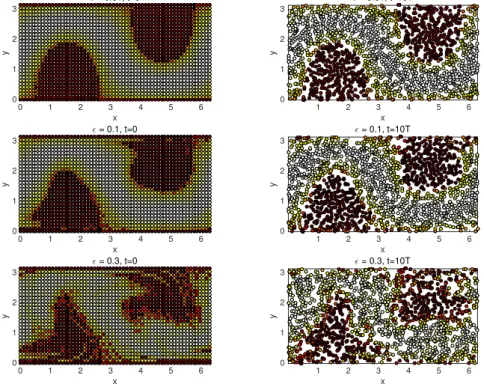
the tracer trajectories taken as observations every 10δttime steps. As shown in Figure1, although changing its shape with ε, the coherent pattern is very persistent in the sense that those initial tracers labelled in similar colours according to the PCA dominant mode are still tightly grouped together and retain their collective geometrical structure after a long period of time; this gives an intuition of what we mean here by the coherent pattern. Note also that, dynamically speaking,
under the small (deterministic) disturbance, the flow is near-integrable and the coherent pattern is determined by the persisting geometry of the circulation regime and jet flowing regime.
0 1 2 3 4 5 6
x 0
1 2 3
y
ǫ = 0.01, t=0
1 2 3 4 5 6
x 0
1 2 3
y
ǫ = 0.01, t=10T
0 1 2 3 4 5 6
x 0
1 2 3
y
ǫ = 0.1, t=0
1 2 3 4 5 6
x 0
1 2 3
y
ǫ = 0.1, t=10T
0 1 2 3 4 5 6
x 0
1 2 3
y
ǫ = 0.3, t=0
1 2 3 4 5 6
x 0
1 2 3
y
ǫ = 0.3, t=10T
Figure 1: Coherent pattern based on the dominant eigenvector of Px1 for various values ofε. Left: initial conditions evenly spaced on a grid. Right: flow at time t= 20.
We now confirm that the coherent pattern can be detected using relatively few tracers, and that the coherent pattern is in this case robust to the noise and chaotic advection in the dynamical
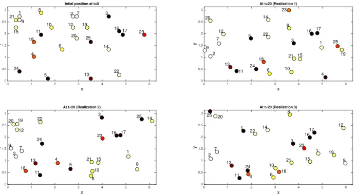
system. We investigate this by limiting the number of tracers to 25, initially randomly placed. We label each tracer and use three realizations of the noise to propagate the tracers to the time
t = 10T. The coherent pattern is again extracted by using the dominant mode of PCA, and the tracers in each of the three realizations are coloured accordingly. We consider PCA to be robust to the chaotic, stochastic dynamics if tracers with the same label have similar colours across each of
the 3 realizations. We show the initial conditions and 3 typical realizations in Figure 2.
We now establish the usefulness of the Hellinger distance as a metric to infer model parameters
0 1 2 3 4 5 6 x 0 0.5 1 1.5 2 2.5 3 y
At t=20 (Realization 1)
1 2 3 4 5 6 7 8 9 10 11 12 13 14 15 16 17 18 19 20 21 22 23 24 25
0 1 2 3 4 5 6
x 0 0.5 1 1.5 2 2.5 3 y
At t=20 (Realization 2)
1 2 3 4 5 6 7 8 9 10 11 12 13 14 15 16 17 18 19 20 21 22 23 24 25
0 1 2 3 4 5 6
x 0 0.5 1 1.5 2 2.5 3 y
At t=20 (Realization 3)
1 2 3 4 5 6 7 8 9 10 11 12 13 14 15 16 17 18 19 20 21 22 23 24 25
0 1 2 3 4 5 6
x 0 0.5 1 1.5 2 2.5 3 y
Intial position at t=0
1 2 3
4 5 6 7 8 9 10 11 12 13 14
15 1617
18 19 20 21 22 23 24 25
Figure 2: The coherent patterns are obtained via PCA for three independent experiments. Top left: initial conditions for the other 3 plots, with tracers labelled 1 to 25. Top right and bottom row: 3 realizations of the tracer locations at t= 20, obtained by numerically integrating (7.1)–(7.2). The realizations are coloured by their PCA dominant mode. We observe that, despite the tracers having very different final locations, the PCA dominant mode tends to assign similar colours to each tracer in all realizations (e.g. tracer 18 is red for all three realizations).
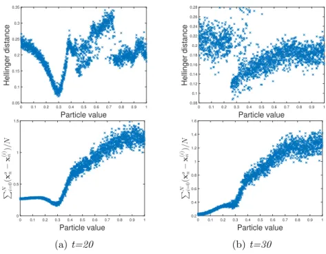
longer has a minimum near the correct value of ε, but the Hellinger distance does. We used 50 drifters deployed in a circle of radius 0.1 around the centres π2,1
, 32π, π−1
of each gyre.
7.2 Data assimilation by SMC-ABC
In this section we explore the robustness of the SMC-ABC algorithm, measured against the standard
particle filter (PF). Following the discussion in Section 1and the results of Figure 3, we define two ‘failure states’ for the PF. We expect the PF to become degenerate when there are many accurately
observed drifters, meaning that one particle will have weight 1 and all other particles will have weight 0. However, we are estimating static parameters; it is quite possible for the (degenerate) particle filter to accurately estimate these parameters with a single particle. We would like to
observe a second failure on the part of the PF, that if the drifters are located in regions of chaotic advection in the model, and if the time between observations is sufficient for the initial observation error to completely separate the simulated drifter trajectories from the true trajectories, then the
PF may be expected to gain no information over the prior guess for the parameter(s).
We focus on estimating the parameters ε, k1, l1, c1 (particularly ε, k1) that characterise the time-dependent peturbation. In order to observe the above failure state in the PF, we will typically initialise the drifters in two rings around the centre of each gyre, and take observations on intervals at leastt= 30. By taking observations on time intervals less than 30, or as we shall see by initialising the drifters uniformly in phase space, the degenerate PF can estimate parameters more accurately than SMC-ABC. It is specifically the robustness of the coherent pattern to chaotic advection that
0 0.1 0.2 0.3 0.4 0.5 0.6 0.7 0.8 0.9 1 Particle value 0.05 0.1 0.15 0.2 0.25 0.3 0.35 Hellinger distance
0 0.1 0.2 0.3 0.4 0.5 0.6 0.7 0.8 0.9 1 Particle value 0.08 0.1 0.12 0.14 0.16 0.18 0.2 0.22 0.24 0.26 0.28 Hellinger distance
0 0.1 0.2 0.3 0.4 0.5 0.6 0.7 0.8 0.9 1 Particle value
0 0.5 1 1.5
PN i
=
0
(
x
o n−
x ( i ) n ) /N (a)t=20
0 0.1 0.2 0.3 0.4 0.5 0.6 0.7 0.8 0.9 1 Particle value 0.2 0.4 0.6 0.8 1 1.2 1.4 1.6
PN i
=
0
(
x
o n−
x ( i ) n ) /N (b)t=30
Figure 3: An experiment was performed in which 50 drifters were numerically integrated by (7.1)–(7.2) using 2000 uniformly spaced values of ε. Each plot shows the particles, i.e. the possible values of ε, plotted against the Hellinger distance (the metric used in SMC-ABC) between simulated and observed patterns, or the distance xo
n−x
(i)
n between simulated and observed drifters, related to the metric used in PF. For an
7.2.1 Experimental setup
In the following experiments, we use a final time of t= 30. The PF and SMC-ABC schemes use a model time step of 0.1, and a single observation is taken at the final time. The observations are synthetically generated from a model integration using a time step of 0.01.
Our observations are of the trajectories of 50 tracers; the initial positions of these tracers are typ-ically circles of radius 0.1 around the centres of each gyre. We construct the “truth” by taking a realization produced by the above parameter values.
We are interested in comparing the performance of PF and SMC-ABC at the same computational
cost. Accordingly, we modify SMC-ABC as follows: we choose the number of particles N in SMC-ABC to be one tenth the number of particles used in the PF. Furthermore, we restrict the SMC-ABC algorithm to at most ten steps in the artificial time n; that is ifn= 10 in Algorithm 1 the While loop is halted and we return the final particle distribution{θ(10i)}. With this modification the computational cost of SMC-ABC is controlled to be roughly equivalent to, or less than, the
cost of PF.
In the following experiments, the transition kernel qn(θ, θ∗) is given by the random walk
θ∗ =θ+η, η∼ N(0,0.01). (7.3)
Therefore, the MH ratio (5.11) is either 0 or 1; the weight of thei−th particle at then−th step is 1 if it has survived allnrejection steps, or if it has been resampled and then survived the intervening rejection steps, and it is 0 otherwise.
7.2.2 One parameter experiments
We perform experiments to estimate the time-dependent peturbation parameter ε, assuming that the prior density π(ε) is a uniform distribution on the interval [0,1].
We investigate how the absolute error
PN i=1θ
(i)
n w(ni)−ε
scales with the number of particles N, when all other parameters are kept fixed. We present results for PF withN ={250,500,1000,2000}
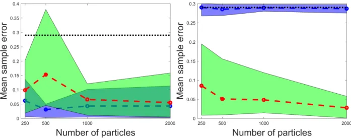
particles, and SMC-ABC with N ={25,50,100,200} particles. As discussed in Section 7.2.1, un-der this set-up SMC will have lesser or equal computational cost to PF, and we overlay the results accordingly. We suppose that the true parameter is ε= 0.3, and present results for two situations, one in which the drifters are initially distributed uniformly and a second in which the drifters are
Figure 4: Error in estimating the peturbation strength εin the PF (blue)and SMC-ABC (green). Circles and dashed lines show the mean error of 20 repetitions from each numerical method, while the coloured patches show the10%and90%percentiles. The black dotted line shows the mean error of the initial distribution of the particles. Left:drifters are initially deployed uniformly, and the Particle Filter (while always degenerate) can accurately estimateε. Right: drifters are initially deployed within the gyres, their trajectories are dominated by chaotic advection, and the Particle Filter gains no information on ε from the drifter locations. In both cases SMC-ABC can infer εfrom the coherent pattern created by the drifters.
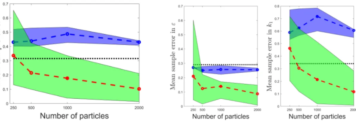
7.2.3 Multiple parameter experiments
In this section we use SMC-ABC and PF to simultaneously estimate the perturbation parameter
ε and the amplitude and frequency parameterk1 in (7.1)–(7.2). We label the set of parameters to be estimated by Θ = (ε, k1), with true values = 0.3 and k1 = 1. We take the prior density π(Θ) to be a uniform distribution on the interval [0,1]×[0.2,1.2].
We investigate how the absolute error
PN i=1θ
(i)
n wn(i)−Θ
scales with the number of particles N, when all other parameters are kept fixed. The drifters are again initialised inside the bound-aries of each gyre, as done previously. We present results for 20 runs each of a PF with N =
{250,500,1000,2000} particles, and SMC-ABC with N = {25,50,100,200} particles. Again we overlay the results in view of their roughly equivalent computational cost. Figure 5 confirms that SMC-ABC can accurately estimate multiple parameters, while again the PF fails to improve over
the prior guess. We remark that the broad spread of the results for SMC-ABC compared to PF is a consequence of the adjustment to the same computational cost; SMC-ABC is (also) a sequential
monte carlo method employing one tenth the number of particles as PF, and consequently outputs particles with relatively high variance.
8
Discussion
This paper presents, to our best knowledge, the first attempt to develop an approach to assimilate the Lagrangian coherent structure for parameter estimation. In contrast to previous research for LaDA, the new approach does not directly use the error statistics of observed positions of
Figure 5: Left: Mean error in estimating parameters in the PF(blue)and SMC-ABC(green). Circles and dashed lines show the mean error of 20 repetitions from each numerical method, while the coloured patches show the 10% and 90% percentiles. The black dotted line shows the mean error of the initial distribution of the particles. Left: Mean error in estimating bothε and k1. Right: Error in estimating the individual
parameters. In both cases the PF performs poorly and SMC-ABC, while having a large variance, improves on the prior guess and can accurately estimate both parameters.
requires a tool that can extract that structure from the trajectory data. The structure is extracted via a machine learning method, which is PCA in the current work, and the assimilation algorithm is based on the Approximation Bayesian computation (ABC), which allows a bayesian inference
to be performed without computing the typically unavailable likelihood function of the coherent structure. However, a distance function must be appropriately designed to measure the discrepancy
between the observed coherent structure and the coherent pattern predicted by the model simulation based on various parameter values. We use the Hellinger distance and empirically demonstrate its robustness in the situation where the underlying flow exhibits chaotic advection and is stochastically
perturbed.
Our numerical experiments demonstrate that this new approach is remarkably superior to the
trajectory-based Lagrangian DA (employing the particle filter) in the situation where the number of tracers is large and the drifter trajectories are dominated by chaotic advection. In order to achieve this situation, we initialised drifters in the chaotic regions of a peturbed jet flow. The
comparison uses the average mean-square error to measure the accuracy of the estimate. The improved accuracy of the ABC approach is attributed in large part to the following facts: (1) the
Hellinger distances for the coherent structure is usually less sensitive to the stochastic perturbation than the likelihood function of tracer trajectories, which is assumed to be highly informative (i.e. to have small variance). (2) Even in the chaotic flow, the large-scale coherent structure is still
geometrically “regular” while the tracer trajectories may experience high dispersiveness due to the stretching and folding process.
We now briefly discuss convergence results for the SMC-ABC algorithm. On the SMC side, [9] discusses how to obtain convergence results for the stochastically resampled SMC scheme by con-necting it to deterministic resampling schemes (convergence results for which are obtained via the
Central Limit Theorem and are given in, for instance, [48]). It may be more difficult to establish convergence for the ABC component, which would typically entail confirming that the coherent
the flow considered in this paper, the coherent pattern is more than just a summary statistic. In
other words, the likelihood function given by the tracer trajectories is different to the likelihood function given by the coherent pattern.
In future work we will examine our approach in the case of transitory coherent sets, which exist for a finite time before losing coherency due to a change of parameters. Detecting the parameter change is of interest in many applications and it will require developing a new algorithm that exploits the
coherent structure to track the change.
9
Acknowledgements
JM is grateful for the support of the MURI grant A100752, ONR grant N00014-15-1-2112, and
NSF grant DMS-1312906. NS acknowledges the support of the Department of Mathematics at Univeristy of Surrey.
References
[1] A. Apte and C. K. R. T. Jones. The impact of nonlinearity in Lagrangian data assimilation.
Nonlinear Proc. Geophys., 20:329–341, 2013.
[2] A. Apte, C. K. R. T. Jones, and A. M. Stuart. A Bayesian approach to Lagrangian data assimilation. Tellus A, 60(2):336–347, 2008.
[3] R. Banisch and P. Koltai. Understanding the geometry of transport: diffusion maps for La-grangian trajectory data unravel coherent sets. arXiv:1603.04709v2, 2016.
[4] M. A. Beaumont, J. M. Cornuet, J. M. Marin, and C. P. Robert. Adaptive approximate Bayesian computation. Biometrika, 86:983–990, 2009.
[5] L. Billing, E. M. Bollt, and I. B. Schwartz. Phase-space transport of stochastic chaos in population dynamics of virus spread. Phys. Rev. Letters, 88:234101, 2002.
[6] E. M. Bollt and N. Santitissadeekorn.Applied and computational measurable dynamics. Math-ematical modeling and computation. SIAM, 2013.
[7] Collecte Localisation Satellites. Argos User’s Manual: Worldwide tracking and environmental
monitoring by satellite, 2007-2016.
[8] Pierre Del Moral. Non-linear filtering: interacting particle resolution. Markov processes and
related fields, 2(4):555–581, 1996.
[9] Pierre Del Moral, Arnaud Doucet, Ajay Jasra, et al. On adaptive resampling strategies for
sequential Monte Carlo methods. Bernoulli, 18(1):252–278, 2012.
[10] M. Dellnitz and O. Junge. Almost invariant sets in Chua’s circuit. Int. J. Bif. Chaos, 7(11):2475–2485, 1997.
[11] M. Dellnitz and O. Junge. On the approximation of complicated dynamical behaviours. SIAM
[12] S. F. Dimarco, W. D. Nowlin, and R. O. Reid. A statistical description of the velocity fields
from upper ocean drifters in the Gulf of Mexico. Geophysical Monograph Series-American
Geophysical Union, 161:101–110, 2005.
[13] Kathleen Dohan, F Beaujean, Luca Centurioni, MF Cronin, Gary Lagerloef, Dong-Kyu Lee,
R Lumokin, Nikolai A Maximenko, Pearn P Niiler, and H Ichida. Measuring the global ocean surface circulation with satellite and in situ observations. Proceedings of the ”OceanObs’09:
Sustained Ocean Observations and Information for Society”, 2, 2010.
[14] David M Fratantoni. North Atlantic surface circulation during the 1990’s observed with
satellite-tracked drifters. Journal of Geophysical Research: Oceans, 106(C10):22067–22093, 2001.
[15] G. Froyland and M. Dellnitz. Detecting and locating near-optimal almost-invariant sets and cycles. SIAM J. Sci. Comput., 24(6):1839–1863, 2003.
[16] G. Froyland, C. Horenkamp, V. Rossi, N. Santitissadeekorn, and A. S. Gupta. Three-dimensional characterisation and tracking of an Agulhas ring. Ocean Modelling, 5253:69–75,
2012.
[17] G. Froyland, O. Junge, and P. Koltai. Estimating long term behaviour of flows without trajec-tory integration: the infinitesimal generator approach. SIAM J. Numer. Anal., 51(1):223–247, 2013.
[18] G. Froyland, S. Lloyd, and N. Santitissadeekorn. Coherent sets for nonautonomous dynamical
systems. Phys. D, 239(16):1527 – 1541, 2010.
[19] G. Froyland and K. Padberg. Almost-invariant sets ad invariant manifolds–connecting
prob-abilistic and geometric descriptions of coherent structures in flows. Physica D, 238(16):1507– 1523, 2009.
[20] G. Froyland and K. Padberg-Gehle. A rough-and-ready cluster-based approach for extracting finite-time coherent sets from sparse and incomplete trajectory data. Chaos, 25(087406), 2015.
[21] G. Froyland, N. Santitissadeekorn, and A. Monahan. Transport in time-dependent dynamical
systems: Finite-time coherent sets. Chaos, 20(4), 2010.
[22] Neil J Gordon, David J Salmond, and Adrian FM Smith. Novel approach to
nonlinear/non-Gaussian Bayesian state estimation. Rad. and Sig. Pro., IEE Proc. F, 140(2):107–113, 1993.
[23] A. Hadjighasem, D. Karrasch, H. Teramoto, and G. Haller. Spectral-clutersing appraoch fo Lagrangian vortex detection. Phys. Rev. E, 93(063107), 2016.
[24] G. Haller. Lagrangian coherent structures from approximate velocity data. Phys. Fluids A, 14:1851–1861, 2002.
[25] K. Ide, L. Kuznetsov, and C. K. R. T. Jones. Lagrangian data assimilation for point vortex
systems. J. Turbulence, 3, 2002.
[27] P. Krause and J. M. Restrepo. The diffusion kernel filter applied to Lagrangian data
assimi-lation. Mont. Weather. Rev., 137:4386–4400, 2009.
[28] K. Law, A. Stuart, and K. Zygalakis. Data Assimilation: Mathematical Introduction. Springer-Verlag, 2015.
[29] L. Liu. Lagrangian data assimilation into layered ocean model. PhD thesis, UNC-CH, Chapel Hill, NC, 2007.
[30] Jean-Michel Marin, Pierre Pudlo, Christian P Robert, and Robin J Ryder. Approximate
Bayesian computational methods. Statistics and Computing, pages 1–14, 2012.
[31] A. Molcard, L. I. Piterbarg, A. Griffa, T. M. Ozgokmen, and A. J. Mariano. Assimilation of
drifter observations for the reconstruction of the Eulerian circulation field. J. Geophys. Res., 108(C3):3056, 2003.
[32] P. Del Moral, A. Doucet, and A. Jasra. Sequential Monte Carlo Samplers. J. R. Stat. Soc. B, 68:411–436, 2006.
[33] P. Del Moral, A. Doucet, and A. Jasra. An adaptive sequential Monte Carlo method for
approximate Bayesian computation. Stat. Comput., 2011.
[34] P. Del Moral and L. M. Murray. Sequential Monte Carlo with highly informative observations.
SIAM/ASA J. on Uncertainty Quant., 3(1):969–997, 2015.
[35] S. Nakano, G. Ueno, and T. Higuchi. Merging particle filter for sequential data assimilation.
Nonlin. Process. Geophys., 14:395408, 2007.
[36] RT Pierrehumbert. Chaotic mixing of tracer and vorticity by modulated travelling Rossby waves. Geophysical & Astrophysical Fluid Dynamics, 58(1-4):285–319, 1991.
[37] J. Poterjoy. A localized particle filter for high-dimensional nonlinear systems. Mon. Weather
Rev., 144:59–76, 2016.
[38] Pierre-Marie Poulain. Adriatic Sea surface circulation as derived from drifter data between
1990 and 1999. Journal of Marine Systems, 29(1):3–32, 2001.
[39] D. Rubin. Bayesianly justifiable and relevant frequency calculations for the applied statistician.
Ann. of Stat., 12(4):1151–1172, 1984.
[40] H. Salman, L. Kuznetsov, C. K. R. T. Jones, and K. Ide. A method for assimilating Lagrangian data into a shallow-water equation ocean model. Mon. Weather. Rev., 134:1081–1101, 2006.
[41] R. M. Samelson and S. Wiggins. Lagrangian transport in geophysical jets and waves: the
dynamical system approach, volume 31 of Interdisciplinary Applied Mathematics. Springer,
New York, 2006.
[43] N. Santitissadeekorn and C. K. R. T. Jones. A bimodality trap in model projections. Chaos,
25(3), 2015.
[44] N. Santitissadeekorn and C. K. R. T Jones. Two-Stage Filtering for Joint State-Parameter Estimation. Mon. Weather Rev., 143:2028–2042, 2015.
[45] P. J. Schmid. Dynamic mode decomposition of numerical and experimental data. J. of Flu.
Mech., 656:5–28, 2010.
[46] S. Sisson, Y. Fan, and M. M. Tanaka. Sequential Monte Carlo without likelihood. Proc. Natl.
Acad. Sci., 104:1760–1765, 2007.
[47] L. Slivinski, E. Spiller, A. Apte, and B. Sandstede. A hybrid particle-ensemble Kalman filter
for Lagrangian data assimilation. Mon. Weather Rev., 143:195–211, 2015.
[48] A Smith, Arnaud Doucet, Nando de Freitas, and Neil Gordon.Sequential Monte Carlo Methods
in Practice. Springer Science & Business Media, 2013.
[49] E. T. Spiller, A. Budhiraja, and C. K. R. T. Jones. Modified particle filter methods for assimilating Lagrangian data into a point-vortex model. Physica D, 237:1498–1506, 2008.
[50] S. Tavar´e, D. Balding, R. Griffith, and P. Donnelly. Inferring coalescence times from DNA sequence data. Genetics, 145(2):505–518, 1997.
[51] T. Tina, D. Welch, N. Strelkowa, A. Ipsen, and M. P. H. Stumpf. Approximate Bayesian
Computation scheme for parameter inference and model selection in dynamical systems. J. R.
Soc. Interface, 6:187–202, 2008.
[52] J. H. Tu, C. W. Rowley, D M. Luchtenburg, S. L. Brunton, and N. J. Kutz. On dynamical mode decomposition: theory and applications. J. of Comput. Dyna., 1(2):391, 2014.
[53] Christopher K Wikle and L Mark Berliner. A Bayesian tutorial for data assimilation. Physica