E
SSAYS INF
INANCIALE
CONOMETRICS ANDM
ACROFINANCEStephen Raymond
A dissertation submitted to the faculty of the University of North Carolina at Chapel Hill in par-tial fulfillment of the requirements for the degree of Doctor of Philosophy in the Department of
Economics.
Chapel Hill 2020
Approved by:
Eric Ghysels
M. Max Croce
Lukas Schmid
Anusha Chari
c
2020
ABSTRACT
STEPHEN RAYMOND: Essays in Financial Econometrics and Macrofinance. (Under the direction of Eric Ghysels)
These three essays focus on various manifestations of risk: collective institutional investor risk, individual retail investor risk, and risk generated by government debt.
In the first essay, we look at how institutional investor concentration can impact downside risk. The U.S. equities market price process is largely driven by the information set and actions of large institutional investors, not individual retail investors. Using quarterly 13-F holdings, we construct the Herfindahl-Hirschman Index (HHI) of institutional investor concentration as a measure of gran-ularity. Our contributions are both empirical and theoretical. We provide a comprehensive study of how granularity affects: (1) the cross-section of returns, (2) conditional variances across stocks and (3) downside risk. We find that constructing a low-HHI minus high-HHI portfolio produces an annualized return of 5.6%. Using an approach advocated by Koijen and Yogo, we document that the cross-section of HHI portfolios can be explained by a conditional asset pricing model involving heterogeneous investor demands driven by time-varying beliefs over asset characteristics. We doc-ument the adverse impact that investor ownership concentration has on both conditional volatility, and critically, a robust set of downside risk measures at both the portfolio and the firm level.
robo-advising. We explore robo-investing strategies commonly used in the industry, including some involving advanced machine learning methods. The man versus machine comparison allows us to shed light on possible benefits the emerging robo-advising industry may provide to certain segments of the population, such as low income and/or low education investors.
ACKNOWLEDGMENTS
TABLE OF CONTENTS
LIST OF TABLES . . . xi
LIST OF FIGURES . . . xvi
1 Granularity and (Downside) Risk in Equity Markets . . . 1
1.1 Introduction . . . 1
1.2 Expected Returns, Volatility and Downside Risk . . . 5
1.2.1 Conditional Means – Linear Factor Models . . . 9
1.2.2 Conditional Volatility . . . 10
1.2.3 Downside Risk . . . 14
1.3 Downside Risk and Top Players . . . 17
1.3.1 Portfolio-Level Downside Risk by Top Players . . . 18
1.3.2 Firm-Level Downside Risk by Top Players . . . 21
1.3.3 Evidence From Options Markets . . . 22
1.3.4 Risk By Investor Characteristics . . . 24
1.4 A Heterogeneous Investor Demand-driven Model . . . 24
1.4.1 Downside Risk in a Stylized Economy . . . 25
1.4.2 Breaking up Large Investors . . . 28
1.4.3 Market Share Restrictions . . . 29
1.4.4 Motivating a Conditional Asset Pricing Model . . . 30
1.5 Conclusion . . . 32
2.1 Introduction . . . 35
2.2 A Large Panel of Individual Brokerage Accounts . . . 39
2.3 Robo-Investors . . . 42
2.3.1 AI Alter Egos . . . 42
2.3.2 Machine Learning Expected Returns . . . 45
2.3.3 Global ETF Robo-investors . . . 49
2.4 Empirical Results . . . 50
2.4.1 Are more sophisticated models better? . . . 50
2.4.2 Who gains from robo-advise? . . . 51
2.4.3 How does robo-advising perform during major financial crisis? . . . 53
2.4.4 AI Alter Egos versus Passive Investments . . . 55
2.4.5 Are the spreads due to market or behavioral factors? . . . 56
2.4.6 AI Enhancements to Passive Investment . . . 57
2.5 Conclusions . . . 58
3 Government Debt and the Returns to Innovation . . . 71
3.1 Introduction . . . 71
3.1.1 Related literature . . . 74
3.2 Empirical analysis . . . 76
3.2.1 Data sources . . . 76
3.2.2 Time-series asset pricing tests . . . 79
3.2.3 Government debt, R&D, and growth . . . 84
3.3 An asset-pricing model with public debt and innovation . . . 90
3.3.1 Government . . . 91
3.3.2 Production . . . 92
3.3.4 Equilibrium and asset prices . . . 96
3.3.5 Aggregate productivity growth and fiscal policy . . . 99
3.4 Quantitative analysis . . . 100
3.4.1 Calibration . . . 100
3.4.2 Findings . . . 103
3.4.3 Findings: debt and innovation returns . . . 106
3.4.4 Sensitivity . . . 113
3.5 Cross-sectional asset pricing tests . . . 114
3.5.1 Conditional model with time-varying betas. . . 114
3.6 Conclusion . . . 116
A Appendix to Chapter 1 . . . 118
A.1 HHI Portfolio Analysis Details . . . 118
A.1.1 Portfolio Construction . . . 118
A.1.2 HHI Decomposition . . . 119
A.1.3 Low-Minus-High (LMH) Portfolio Characteristics . . . 119
A.1.4 Equally-Weighted Linear Factor Model Details . . . 121
A.2 Pre-Crisis Period . . . 123
A.2.1 Downside Risk . . . 123
A.2.2 Downside Risk with Decomposed HHI . . . 124
A.3 Value-Weighted Portfolio . . . 128
A.4 Top Players - Dynamic Specifications . . . 137
A.5 HHI Decomposed By Investor Characteristics . . . 140
A.6 Reduced Form Model Details . . . 142
B Appendix to Chapter 2 . . . 143
B.1.1 Portfolios and Individual Investor Characteristics . . . 144
B.1.2 Sample of stocks and ETFs . . . 146
B.1.3 Sample of investors . . . 148
B.1.4 Behavioral Biases . . . 154
B.1.5 Individual investor returns adjusted for cash holding . . . 155
C Appendix to Chapter 3 . . . 183
C.1 Additional statistics and tests . . . 183
C.2 Tax rate dependence on the debt-to-output ratio . . . 198
C.3 Empirical specifications . . . 200
C.3.1 Parameterizedβregressions . . . 200
C.3.2 TFP construction . . . 200
C.3.3 Look-ahead bias correction . . . 200
C.3.4 Stambaugh bias correction . . . 201
C.3.5 Characteristic-adjusted returns . . . 201
C.3.6 Monte Carlo evidence . . . 201
LIST OF TABLES
1.1 Annualized HHI Low-High Portfolio Returns . . . 8
1.2 Linear Factor Correlations . . . 9
1.3 HHI Portfolios Unconditional Linear Factor Models . . . 10
1.4 Conditional Volatility Regressions – Quarterly . . . 12
1.5 Conditional Volatility Regressions – Monthly . . . 13
1.6 Regression of Conditional Quantile on HHI . . . 15
1.7 Top Institutions Holding Decomposition . . . 18
1.8 Regression of Conditional Quantile on Decomposed HHI . . . 20
1.9 Firm-Level Risk on Investor Concentration Regressions . . . 23
1.10 Regression of Conditional Quantile on HHI: Simulated Data . . . 28
1.11 Impact of Uncertainty on Conditional Betas . . . 33
1.12 Conditional Asset Pricing Model . . . 33
2.1 Out-of-Sample MSE Across Stocks . . . 63
2.2 AI Alter Ego Return Spreads - All Investors . . . 64
2.3 Ranked Variables Based on Relative`2Contribution Across Stocks . . . 65
2.4 AI Alter Egos Return Spreads - Education, Risk Aversion and Income . . . 66
2.5 Returns Pre-Crisis, Crisis and Post-Crisis . . . 67
2.6 AI Alter Ego Return Spreads vis-`a-vis benchmark ETFs . . . 68
2.7 Disposition Effect and AI Alter Ego Return Spreads - Median regression . . . 69
2.8 Return Spreads Global ETF Robo-investors minus Realized Cash-Adjusted . . . . 70
3.1 Portfolio Summary Statistics . . . 78
3.4 Predicting Changes in Investment with∆DGDP . . . 87
3.5 DGDP and Growth Predictability . . . 89
3.6 Benchmark Calibration . . . 102
3.7 Model Summary Statistics . . . 104
3.8 Predictive Regressions:DGDP . . . 107
3.9 Conditional Macro Factors Model . . . 117
A.1 Portfolio HHI Summary Statistics . . . 119
A.2 Portfolio HHI Decomposition . . . 120
A.3 Annualized Portfolio Returns . . . 120
A.4 Liquidity-Risk Adjusted Excess Returns . . . 121
A.5 Conditional Mean Linear Factor Models . . . 122
A.6 Regression of Conditional Quantile on HHI: Pre-crisis . . . 123
A.7 Regression of Conditional Quantile on Quarterly HHI - Pre-crisis . . . 124
A.8 Regression of Conditional Quantile on Decomposed HHI - Pre-crisis . . . 125
A.9 Regression of Conditional Quantile on Quarterly Decomposed HHI - Pre-crisis . . 126
A.10 Regression of Conditional Quantile on HHI - First Month Pre-crisis . . . 127
A.11 Annualized HHI Low-High Portfolio Returns - VW . . . 128
A.12 Annualized Portfolio Returns – VW . . . 128
A.13 Liquidity-Risk Adjusted Excess Returns – VW . . . 128
A.14 Conditional Mean Linear Factor Models - VW . . . 129
A.15 Conditional Volatility Regressions – Quarterly – VW . . . 130
A.16 Conditional Volatility Regressions – Monthly – VW . . . 130
A.17 Regression of Conditional Quantile on HHI, Value-Weighted . . . 132
A.18 Regression of Conditional Quantile on Decomposed HHI, Value-Weighted . . . . 133
A.20 Regression of Conditional Quantile on Quarterly HHI - Pre-crisis, Value-Weighted 134
A.21 Regression of Conditional Quantile on Decomposed HHI - Pre-crisis, Value-Weighted
. . . 135
A.22 Regression of Conditional Quantile on Quarterly Decomposed HHI - Pre-crisis, Value-Weighted . . . 136
A.23 Regression of Conditional Quantile on HHI - Quarterly . . . 137
A.24 Regression of Conditional Quantile on Decomposed HHI - Quarterly . . . 138
A.25 Regression of Conditional Quantile on HHI - First Month . . . 139
A.26 Composition of HHI Portfolios by Investor Characteristics . . . 140
A.27 Conditional Volatility by HHI Decomposition by Investor Type . . . 141
A.28 Conditional Volatility by HHI Decomposition by Investor Classification . . . 141
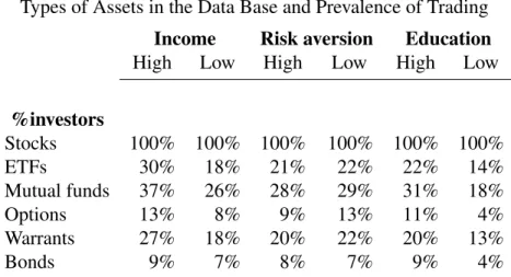
B.1 Types of Assets in the Data Base and Prevalence of Trading . . . 144
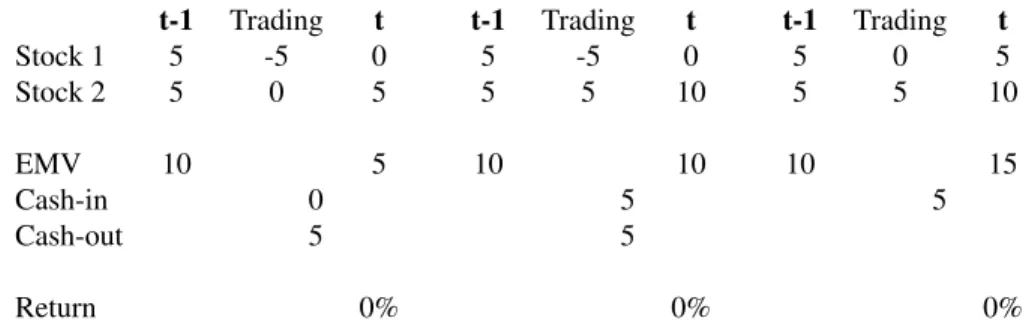
B.2 Illustrative Examples of Cash Flows and Return Computations . . . 145
B.3 International Coverage of Stocks . . . 147
B.4 Stock Distribution Across Industry Sectors . . . 147
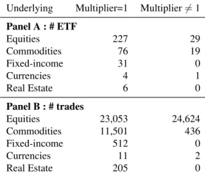
B.5 Statistics About ETFs Underlying Assets . . . 148
B.6 ETFs Top 5 . . . 148
B.7 Cross-sectional Statistics for Asset Prices, Monthly Returns and Risk Factors . . . 149
B.8 Investor Characteristics Joint Percentages . . . 150
B.9 Cross-Sectional Statistics for Investors’ Age, Monthly Trading Activity and Portfolio151 B.10 Statistics for ETFs usage . . . 152
B.11 Summary Statistics Disposition Effect . . . 153
B.12 Summary Statistics Monthly Trading Frequency Stocks and ETFs . . . 154
B.13 Returns Monthly Rebalancing . . . 157
B.14 Returns Monthly Rebalancing - Education-Sorted . . . 158
B.16 Returns Monthly Rebalancing - Income-Sorted . . . 160
B.17 AI Spreads Monthly Rebalancing . . . 161
B.18 AI Spreads Equities & ETFs Monthly Rebalancing - Education-Sorted . . . 162
B.19 AI Spreads Equities & ETFs Monthly Rebalancing - Risk Aversion-Sorted . . . 163
B.20 AI Spreads Equities & ETFs Monthly Rebalancing - Income-Sorted . . . 164
B.21 Returns Quarterly Rebalancing . . . 165
B.22 AI Spreads Quarterly Rebalancing . . . 166
B.23 AI Spreads Equities & ETFs Quarterly Rebalancing - Education-Sorted . . . 167
B.24 AI Spreads Equities & ETFs Quarterly Rebalancing - Risk Aversion-Sorted . . . . 168
B.25 AI Spreads Equities & ETFs Quarterly Rebalancing - Income-Sorted . . . 169
B.26 Summary Statistics Returns - Equities & ETFs - Pre NBER Crisis . . . 170
B.27 AI Spreads - Equities & ETFs - Pre NBER Crisis . . . 171
B.28 Summary Statistics Returns - Equities & ETFs - During NBER Crisis . . . 172
B.29 AI Spreads - Equities & ETFs - During NBER Crisis . . . 173
B.30 Summary Statistics Returns - Equities & ETFs - Post NBER Crisis . . . 174
B.31 AI Spreads - Equities & ETFs - Post NBER Crisis . . . 175
B.32 Hypothesis Tests Median . . . 176
B.33 Disposition Effect and Alter Ego Spreads - Quantile Regressions . . . 177
B.34 Disposition Effect and Alter Ego Spreads vis-`a-vis S&P 500 ETF - Quantile Re-gressions . . . 178
B.35 Individual Investors Benefiting from Robo-Investing . . . 179
B.36 Monthly trading activity and portfolio depending on investor income . . . 180
B.37 Monthly trading activity and portfolio depending on investor risk aversion . . . 181
B.38 Monthly trading activity and portfolio depending on investor education . . . 182
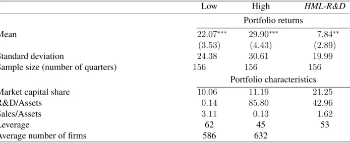
C.1 Top 10 Industries in R&D Intensity Sorted Portfolio . . . 183
C.3 Data Summary Statistics – Positive R&D Firms . . . 185
C.4 Portfolio Summary Statistics – Allocated by Number of Firms . . . 186
C.5 Tstat by Newey-West Lags – HML R&D Returns . . . 187
C.6 Predictive Regression for HML-R&D – Additional Factors . . . 187
C.7 Predictive Regressions - HML-R&D Adjusted Returns . . . 188
C.8 DGDP and Predictability of Returns to Innovation . . . 189
C.9 DGDP and Predictability of Returns to Innovation (Positive R&D Firms-EW) . . . 190
C.10 PD, MVand Predictability of Returns to Innovation (Pos. R&D Firms-EW) . . . 191
C.11 DGDP and Predictability of Returns to Innovation (Positive R&D Firms-VW) . . 192
C.12 PD, MVand Predictability of Returns to Innovation (Pos. R&D Firms-VW) . . . . 193
C.13 DGDP and Predictability with Annual Re-balance . . . 194
C.14 Conditional Macro Factors Model (II) . . . 195
C.15 Conditional Macro Factors Model – Positive R&D Firms . . . 196
C.16 Conditional Macro Factors Model – Financially Constrained Adjusted Returns . . . 197
C.1 Avg. Tax Rate in High and Low Debt/GDP Environments . . . 199
LIST OF FIGURES
1.1 Quarterly Top Institutional Investor Market Shares . . . 6
1.2 Quarterly Aggregate HHI . . . 7
1.3 Conditional Volatility High versus Low HHI Portfolio . . . 11
1.4 Conditional Quantile Estimates HHI Portfolios 5% Left Tail . . . 15
1.5 Conditional Quantile Estimates HHI Portfolios 5% Left Tail - GARCH(1, 1) Fil-tered . . . 16
1.6 Conditional Quantile Estimates HHI Portfolios 5% Left Tail - GJR-GARCH(1, 1) Filtered . . . 17
1.7 Rolling WindowβEstimates of Market Excess Return . . . 31
2.1 Percentage of Stocks for Chosen Best-Predictor Model . . . 59
2.2 Out-of-sample MSE Histogram by Model . . . 60
2.3 Risk Aversion Sorted Performance Scatter Plots . . . 61
2.4 Cumulative Returns . . . 62
2.5 Percentage of Negative Expected Returns . . . 63
3.1 US Annual DGDP . . . 79
3.2 Fitted Parameterized DGDP Coefficients . . . 85
3.3 Conditional Risk Premiums . . . 108
3.4 SDF Impulse Responses to Fundamental Shocks . . . 110
3.5 Conditional Tax Risk, Investment Reallocation, and Asset Prices . . . 111
A.1 Quarterly Number of Institutional Investors . . . 118
A.2 Quarterly Institutional Investment Manager Holdings . . . 119
A.3 Conditional Volatility High versus Low HHI Portfolio – VW . . . 131
B.1 Scatter Plot of Realized Returns versus AI Alter Ego . . . 143
B.2 Monthly Return Performance With/Without Cash . . . 155
CHAPTER 1
GRANULARITY AND (DOWNSIDE) RISK IN EQUITY MARKETS (JOINT WITH ERIC GHYSELS AND HANWEI LIU)
1.1 Introduction
The U.S. equities market price process is largely driven by the information sets and actions of large institutional investors, not individual retail investors. As the majority of equity trading vol-ume has moved toward electronic exchanges and higher frequency trading platforms, the influence of a few can have an out-sized influence on the many. This influence may be largely asymmetric in nature, with the degree of institutional impact unevenly distributed among traded names and therefore generating a cross-sectional distribution of risk. We aim to systematically study how institutional investor concentration impacts the conditional distribution of stock returns.
Our analysis touches on the notion ofgranularity. Gabaix (2011) finds that idiosyncratic move-ments in the production of the largest 100 firms explain about one third of the variations in output and Solow residual, suggesting that the granular composition of the economy matters. Carvalho and Gabaix (2013) take this a step further and argue that the so-called “great moderation”, a sig-nificant fall in the volatility of GDP that began in the 1980s, is mostly due to a change in the fluctuations of the output of the biggest firms in the U.S. Both papers pertain to the structure of the economy. Kelly, Lustig, and Van Nieuwerburgh (2013) relate customer-supplier connectedness to firm stock market volatility.
part of a dynamic network.
A number of papers have studied the impact of institutional investors on asset prices, including Shleifer (1986), Morck, Shleifer, and Vishny (1988), Chen, Hong, and Stein (2002), Barberis, Shleifer, and Wurgler (2005), among others. More recently, Ben-David, Franzoni, Moussawi, and Sedunov (2016) also note that the U.S. asset management industry has become increasingly concentrated and study the fact that large institutions are not equivalent to a collection of smaller independent entities. They study the impact of large institutional ownership on stock volatility and find that their presence increases price instability.
We use quarterly 13-F holdings reported by institutional investors and focus on the Herfindahl-Hirschman Index (HHI) as the measure of granularity and provide a comprehensive study of how it affects: (1) the cross-section of returns, (2) conditional variances across stocks and (3) downside risk. We find that forming equally weighted portfolios based on HHI and constructing a low-HHI minus high-low-HHI portfolio produces an annualized return of 5.6%, and a 6.2% liquidity risk-adjusted return. In other words, stocks with significantly concentrated investor bases command an
insurance premium. What might explain this? Is it related to liquidity, i.e. investor concentration and liquidity go hand in hand? We find that the first PC of a HHI low minus high portfolio has a small negative correlation with the excess return on the market portfolio, and only weak positive correlation with the SMB portfolio or the Pastor and Stambaugh (2003a) liquidity factor. When we estimate various factor models, such as the Fama-French three factor model augmented with the aforementioned liquidity factor, we find that the aforementioned HHI premium remains largely un-explained. The evidence regarding the cross-section of expected returns based on value-weighted portfolios is, in contrast, much weaker. However, the findings regarding conditional variance and downside risk, to which we turn next, are robust at the portfolio level - equally- or value-weighted - as well as the individual firm level.
from our analysis that the findings of Ben-David et al. (2016) do appear to prevail at the portfolio return level. In addition to the impact of ownership concentration on conditional volatility at the portfolio level, we find extremely strong evidence of its impact ondownsiderisk. We also exam-ine what happens to our findings if we separate the holdings of the largest institutions from the remaining institutions. This separation reveals the distinct role played by the former. Finally, we also conduct our analysis at the firm level, reinforcing our results at the portfolio level.
an informational cost with having to disclose a large ownership position. In this scenario we also find that imposing this cost significantly mollifies the impact of increasing HHI on the downside risk for the high HHI asset. We caution that this is not a statement about welfare. Rather these relatively simple mechanisms for regulating investors either through crudely redistributing an in-vestor’s capital or directly restricting asset ownership with a tangible cost placed on market share, both serve to ease the impact of HHI on downside risk for those assets already experiencing higher levels of investor concentration.
The structure of the paper is as follows. Section 1.2 outlines the data and empirical results. Section 1.3 highlights the potential impact of the largest asset managers on the market granularity results. Section 1.4 introduces a simulated reduced form model capable of mimicking the empirical findings and discuss the motivating conditional asset pricing model. Section 1.5 concludes.
1.2 Expected Returns, Volatility and Downside Risk
We start with a comprehensive empirical study of investor concentration and its impact on the cross-section of expected returns, individual stock volatility and downside risk. To that end we study the quarterly 13-F holdings reported by institutional investors. We obtain institutional 13-F filings from the Thomson-Reuters Institutional Holdings Database. This database provides owner-ship information of institutional investment managers with assets under management of over $100 million in Section 13(f) securities. These securities, per SEC stipulations, generally include equity securities that trade on an exchange, certain equity options and warrants, shares of closed-end in-vestment companies, and certain convertible debt securities. We also collect quarterly individual stock returns and accounting information from CRSP and COMPUSTAT, respectively. The sample period is from 1980Q1 to 2014Q4. In addition, we collect CRSP daily stock return data for the same period and monthly Fama-French 3 factor return data are obtained through Kenneth French’s website. The Pastor and Stambaugh (2003a) tradable liquidity factors are obtained through WRDS also at the monthly frequency. We transform these monthly return factors into quarterly data. A more detailed analysis of the data appears in the Appendix A.1.
A casual overview of the market composition reveals that, during the 140 quarters or 35-year time period of our sample, there was an upward trend in both the number of 13-F institutional investors and their aggregate dollar holdings. The reported number of institutional investors is 467 in 1980Q1, and increases to 3,750 in 2014Q4. The dollar amount held by the 13-F institutions increased from $321 billion in 1980Q1 to $17.4 trillion in 2014Q4 with several substantial drops in the early 2000s and during the global financial crisis (see Figure A.2 in Appendix A.1).
managers as one entity, and describe their associated holding characteristics vis-`a-vis the universe of all 13-F institutional investor filings.1 The analysis is conducted on a quarterly basis and Figure 1.1 plots the share of holdings by the largest 3, 5, 7 and 10 institutional investors. We observe that by the end of 2014, the 10 largest institutional investors make up 31.11% of all 13-F institution holdings. The proportion is 17.45%, 22.11%, and 26.12% for the top 3, 5, and 7 institutions, re-spectively. These are remarkably different from the market shares at the beginning of 1980, which are 8.31%, 11.50%, 14.28%, and 18.11% respectively for the 3, 5, 7, and 10 largest institutional investors.
FIG. 1.1: Quarterly Top Institutional Investor Market Shares
To proceed with our analysis on market granularity we start by calculating the market-wide Herfindahl-Hirschman Index (HHI), defined as:
HHIt = Nt X
i=1
s2it, (1.1)
wheresitis the market share of institution i during quartert, andNtis the total number of
institu-tional investors during quartert.Figure 1.2, which displays the quarterly aggregate HHI measures, reveals that market concentration was rising steadily until the financial crisis. The market became less concentrated during the financial crisis, but has surpassed its previous level of concentration once the crisis ended. Note that due to the large number of existing institutions, the magnitude of the HHI index remains small.
FIG. 1.2: Quarterly Aggregate HHI
To form portfolios we compute a similar HHI measure that depicts the dispersion of institu-tional ownerships at the individual stock level. Namely, for each listed securitye,we catalog the investment managers that are long in the stock. We record the fractions of these holding sizes relative to the combined holdings of the qualified 13-F institutions, namely:
Hte=
Ne t X
i=1
[seit]2, e= 1, . . . , Et (1.2)
where se
it is the market share of institution i for stock e at timet andNte is the total number of
institutional investors during quartertholdinge=1, . . . , Et,where the latter is the total of equities
manager at the time of the 13-F filings. Alternatively, 100 institutional investors each possessing an equal amount of a stock generates an HHI value of 0.01. The latter signifies a more diverse profile of stock ownership.
The cross-section of stocks is sortable by ownership concentration He
t (see Appendix A.1.1
for details and portfolio summary statistics). We start with equally-weighted portfolios and report descriptive statistics of the low minus high (LMH) HHI portfolios in Table 1.1. These portfolios are long in broad ownership stocks and short in stocks held by few institutional investors. The excess returns are presented in annualized percentages. The LMH portfolios delivers on average a 5.6% annualized excess return, significantly different from 0 at the 1% level. The median return is higher at 7.8% although the distribution is negatively skewed and has a standard deviation of roughly 11%.2
TABLE1.1: Annualized HHI Low-High Portfolio Returns
Mean Median Std. Dev. Skew Kurt. 25 % 75 %
5.57 7.76 11.04 -5.99 57.33 -0.75 14.25
Notes: This table shows summary statistics of annualized percentage returns from the Low-Minus-High (LMH) portfolio we constructed. Quarterly sample starts in 1980Q1 and ends in 2014Q4.
In Appendix A.3 we explore the value-weighted HHI portfolios. The results reported in Table A.11 reveal that the HHI LMH spread is not as impressive with value-weighted portfolios. It has a mean of 76 basis points and is not significant. Hence, the findings reported in Table 1.1 are not robust in terms of a value- versus equally-weighted portfolio scheme. In contrast, almost all of the findings reported in the remainder of the paper - as will be discussed in detail - are robust to the choice of portfolio weighting scheme. In addition, we will also report findings based on individual stocks, by-passing the portfolio formation step.
2In Appendix A.1.3 we also calculate a liquidity-risk adjusted excess returns. The LMH portfolio returns are quite
1.2.1 Conditional Means – Linear Factor Models
How much are HHI portfolio returns explained by standard asset pricing factors? To answer this question we consider a number of factor model specifications, whereFtwill denote the
fac-tor(s). In particular, we consider: (a) the Fama-French 3 Factor model (Rm−Rf, SM B, HM L), (b) Fama-French 3 Factor + Pastor-Stambaugh tradable liquidity (the latter denoted LIQ) and finally (c) Fama-French 3 Factors, Pastor-Stambaugh tradable liquidity and the first principle com-ponent of [HHI]i,t, denotedP C −HHI.We start with the correlation across the factors being
TABLE1.2: Linear Factor Correlations
Rm-Rf SMB HML Liq HHI
Rm-Rf 1.00
-SMB 0.46 1.00
HML -0.20 -0.01 1.00
Liq -0.07 -0.03 -0.01 1.00
HHI -0.07 0.20 0.08 0.18 1.00
Notes:This table shows correlations between (1) Fama-French 3 factors, i.e. market risk, size, and book-to-market, (2) Pastor-Stambaugh tradable liquidity, and (3) first principle component of HHI. Quarterly sample starts in 1980Q1 and ends in 2014Q4.
considered, which appear in Table 1.2. Of particular interest is the first PC-HHI. It has a small neg-ative correlation with the excess return on the market portfolio, and maximal correlation of only 20% with the SMB portfolio. This means that the breadth of institutional ownership is somewhat related to the small cap premium, but that relationship is weak. The same applies to the liquidity factor, with second largest correlation of 18%. The main take-away is that the tradable liquidity factor and the first principle component of HHI are not highly correlated.
Next, we estimate linear factor models of the following form using GMM for the 5 HHI-sorted portfolios at the quarterly frequency from 1980Q1-2014Q4 (i= 1, ...,5,t= 1, ...,139):
Ri,t =αi+Ft0βi+i,t (1.3)
E[Ri,t] =λ0βi+ei
and prices of risk for the HHI portfolios appear in Table A.5 in Appendix A.1.4.3 Companion results for value-weighted portfolios appear in Table A.14 in Appendix A.3. Table 1.3 shows that that none of the proposed factor models sufficiently describe the cross-section of equally-weighted HHI portfolio returns, as evidenced by the rejection of the Gibbons, Ross, and Shanken (1989) test and over-identification J-tests. Moreover, the HHI LMHαis of similar magnitude to its annualized unconditional average of 5.6%. Overall these results also hold to a lesser degree for value-weighted HHI portfolios. Standard unconditional linear factor models do not adequately the cross-section formed on HHI.
TABLE1.3: HHI Portfolios Unconditional Linear Factor Models
CAPM FF3 FF3+Liq q-Factor
HHI LMHα 4.91∗∗∗ 5.51∗∗∗ 6.03∗∗∗ 5.08∗∗ (1.92) (1.86) (1.89) (2.58) GRS p-value (%) <0.01 <0.01 <0.01 <0.01 J-stat p-value (%) 4.68 <0.01 <0.01 <0.01
Notes:This table shows the HHI LMH portfolioα(annualized percentage) as well as the p-values for the Gibbons et al.
(1989) test (GRS) and GMM J-statistic. The tests respectively come from a time-series and 2-step GMM estimation of the following unconditional linear factor models using the HHI-sorted portfolios: CAPM, Fama-French three-factor (FF3), Fama-French three-factor and Pastor-Stambaugh tradable liquidity factor (FF3+Liq), and the Hou-Xue-Zhang q-factor (Hou, Xue, and Zhang (2015b)). Our quarterly sample starts in 1980Q1 and ends in 2014Q4. Newey and West (1987a) standard errors are in parentheses. One, two, and three asterisks denote significance at the 10%, 5%, and 1% levels, respectively.
1.2.2 Conditional Volatility
It was noted that Ben-David et al. (2016) study whether large institutional ownership has a significant impact on individual stock volatility. They conjecture as a potential channel for this effect that large institutions generate higher price impact than smaller institutions. They provide empirical supporting evidence and argue that the effect of large institutions on volatility is unlikely to be related to improved price discovery, because the stocks owned by large institutions exhibit stronger price inefficiency.
We take a slightly different route and estimate GJR-GARCH(1,1) models at the quarterly fre-quency for the high-HHI and low-HHI portfolios. In particular, we estimate the following model:
ri,t = µ+ σi,ti,t, with σ2i,t = a0 + a1σ2i,t−1 + b12i,t−1 + c1I(i,t−1 < 0)2i,t−1. Results for equally-weighted portfolios are reported in the main body of the paper and Appendix A.3 has the value-weighted portfolio findings.
1980Q1 1985Q1 1990Q1 1995Q1 2000Q1 2005Q1 2010Q1 2015Q1
5 10 15 20 25 30 35
Conditional Annualized Volatility in %
High HHI Low HHI
FIG. 1.3: Conditional Volatility High versus Low HHI Portfolio
The estimated conditional volatilities are plotted in Figure 1.3. We observe a clear level shift in the volatilities of the two respective portfolios, suggesting that there is a potential difference in both the average level of volatility as well as the volatility of volatility. The volatility of the high-HHI portfolio is substantially higher, sometimes three to four times the level of annualized volatility of the low-HHI portfolio.4 How much is this due to say small firm effects or other factors affecting the overall level of volatility?
To investigate this further we regress the estimated conditional volatilities on each portfolio’s
4Value-weighted portfolios feature lower portfolio volatilities, but the wedge between high and low HHI portfolios
TABLE1.4: Conditional Volatility Regressions – Quarterly Constant σˆ2
i,t−1 HHI LIQ SMB R2
1 (high HHI)−0.0033 0.4453∗∗∗ 0.0054∗ 0.2158
(0.0028) (0.1571) (0.0030)
5 (low HHI) 0.0011∗∗ 0.4128∗∗∗−0.0079 0.1750
(0.0005) (0.0575) (0.0100)
1 (high HHI)−0.0035 0.4450∗∗∗ 0.0056 −0.0013 0.2162
(0.0031) (0.1408) (0.0034) (0.0075)
5 (low HHI) 0.0011∗∗ 0.4222∗∗∗−0.0079 −0.0010 0.1800
(0.0005) (0.0705) (0.0097) (0.0016)
1 (high HHI)−0.0063∗∗ 0.5029∗∗∗ 0.0085∗∗ −0.0023 −0.0256∗∗∗ 0.3221
(0.0032) (0.1394) (0.0035) (0.0066) (0.0066)
5 (low HHI) 0.0010∗∗ 0.5198∗∗∗−0.0070 −0.0013 −0.0062∗∗∗ 0.2954
(0.0005) (0.0724) (0.0095) (0.0015) (0.0014)
Notes: This table shows estimation results for the regressions in (A.4). Quarterly sample starts in 1980Q1 and ends in 2014Q4. Standard errors are in parentheses. One, two, and three asterisks denote significance at the 10%, 5%, and 1% levels, respectively. Newey and West (1987a) standard errors appear in parentheses.
HHI value, namely fori= 1 and 5 we estimate the following:
ˆ
σi,t2 = bi,0+bi,1ˆσ2i,t−1+bi,2HHIi,t+vi,t (1.4)
ˆ
σi,t2 = bi,0+bi,1ˆσ2i,t−1+bi,2HHIi,t+bi,3Liqt+vi,t
ˆ
σi,t2 = bi,0+bi,1ˆσ2i,t−1+bi,2HHIi,t+bi,3Liqt+bi,4SM Bt+vi,t
where σˆ2
i,t are fitted conditional volatilities from the GJR-GARCH(1,1) estimation.5 The results
appear in Table 1.4. We find that for high-HHI portfolios, increasing investor concentration is as-sociated with higher conditional volatilty, even after controlling for liquidity and size. Conversely, the impact of HHI is statistically insignificant across all specifications for the low-HHI portfolio. In short, marginal increases in investor concentration are associated with higher conditional volatiltiy for stocks with high investor concentration. In other words, the impact of HHI on conditional volatility is asymmetric with respect to the level of HHI (and the findings reported in Table A.15 show this is also true for value-weighted portfolios).
5The lagged dependent variable, being an estimated proxy, may be a cause of concern as it produces a bias forb
i,1
In addition, we estimate GJR-GARCH(1,1) models at the monthly frequency and retain these monthly conditional volatility estimates for the first month in each calendar quarter (January, April, July, and October). We do this to sharpen our focus on the potential impact of HHI immediately following its filing each quarter. We then estimate the same regression specifications and find that the impact of HHI on conditional volatility is similar. Increasing investor concentration is associated with higher conditional volatility in high-HHI portfolios. In addition the point estimates on HHI for the high-HHI portfolios are slightly larger than the quarterly specification, an indication that the impact of HHI each period may dissipate towards the end of the quarter. Equally-weighted portfolio results appear in Table 1.5 whereas value-weighted ones appear in Table A.16. Overall we find that the results of Ben-David et al. (2016) are sufficiently strong to prevail at the portfolio return level.
TABLE1.5: Conditional Volatility Regressions – Monthly
Constant σˆ2
i,t−1 HHI LIQ SMB R2
1 (high HHI)−0.0060 0.4189∗∗∗ 0.0096∗∗ 0.2106
(0.0043) (0.1308) (0.0048)
5 (low HHI) 0.0047∗∗∗ 0.1234 −0.0409 0.0246
(0.0017) (0.1137) (0.0353)
1 (high HHI)−0.0062 0.4170∗∗∗ 0.0098∗ −0.0017 0.2107
(0.0045) (0.1317) (0.0050) (0.0073)
5 (low HHI) 0.0048∗∗∗ 0.1314 −0.0438 0.0067 0.0326
(0.0018) (0.1118) (0.0359) (0.0047)
1 (high HHI)−0.0065 0.4147∗∗∗ 0.0101∗∗ −0.0014 −0.0093 0.2136
(0.0045) (0.1342) (0.0051) (0.0074) (0.0073)
5 (low HHI) 0.0044∗∗∗ 0.1587 −0.0391 0.0062 0.0123 0.0487
(0.0017) (0.1038) (0.0345) (0.0048) (0.0107)
1.2.3 Downside Risk
Arguably the strongest impact of institutional investor concentration appears to be in downside risk.6
We start with estimating conditional quantiles. The model we rely on to characterize down-side risk is the conditional autoregressive value at risk (CAViaR) model introduced by Engle and Manganelli (2004). The functional form is
qt(θ) =β1+β2qt−1(θ) +β3|rt−1|+t,θ, (1.5)
where qt(θ) denotes the conditional quantile associated with probability level θ. We look at θ =
.05, i.e. the left 5% tail. We compute quantiles for each of the HHI portfolios, and the results for the highest HHI and the lowest HHI portfolio appear in Figure 1.6. We clearly see that the high-HHI portfolio has a more pronounced left tail - with values as low as -15%. In fact, the high-high-HHI quantiles are remarkably lower than the ones from the low-HHI portfolio at almost all times. The spread between the high-HHI and low-HHI conditional percentiles is typically on the order of 4 to 5 %.7 We project the estimated quantiles again on the same variables, namely fori= 1 and 5 we run the following regressions:
qi,t(.05) = bi,0+bi,1HHIi,t−1+vi,t (1.6)
qi,t(.05) = bi,0+bi,1HHIi,t−1+bi,2Liqt−1+vi,t
qi,t(.05) = bi,0+bi,1HHIi,t−1+bi,2Liqt−1+bi,3SM Bt−1+vi,t
The results appear in Table 1.6. We find overwhelming evidence that downside risk is driven by the HHI measure in the high but not the low portfolio. This means that stocks with only a
6Since downside risk is much affected by the recent financial crisis, we also report for the purpose of robustness in
a separate Appendix section A.2 results for a pre-crisis sample. Those results indicate that our findings are not driven by the financial crisis.
7Figure A.4, covering value-weighted portfolios, features different patterns for the quantiles but a similar spread
FIG. 1.4: Conditional Quantile Estimates HHI Portfolios 5% Left Tail
TABLE1.6: Regression of Conditional Quantile on HHI
Constant HHI LIQ SMB R2
1 (high HHI) 0.0622 * -0.1614 *** 0.2039
(0.0262) (0.0272)
5 (low HHI) -0.0480 *** 0.1214 0.0014
(0.0131) (0.2785)
1 (high HHI) 0.0630 * -0.1624 *** 0.0045 0.2042
(0.0265) (0.0276) (0.0217)
5 (low HHI) -0.0474 *** 0.1177 -0.0237 0.0063
(0.0131) (0.2789) (0.0286)
1 (high HHI) 0.0680 * -0.1678 *** 0.0060 0.0361 0.2138 (0.0267) (0.0279) (0.0217) (0.0279)
5 (low HHI) -0.0475 *** 0.1183 -0.0236 0.0032 0.0064 (0.0132) (0.2800) (0.0288) (0.0371)
FIG. 1.5: Conditional Quantile Estimates HHI Portfolios 5% Left Tail - GARCH(1, 1)
Filtered
few institutional investors feature an incremental downside risk. Note also how the R2 of the regressions increase for all the high-HHI quantiles, meaning that HHI explains a substantial part of the variation in downside risk.8
To account for volatility when addressing downside risk, we filter the returns through a stan-dard GARCH(1, 1) and a GJR-GARCH(1, 1) model separately. These two scenarios reflect a fair representation of both symmetric and asymmetric GARCH models. We then proceed to use the filtered return series to re-estimate the 5% conditional quantiles, having controlled for conditional volatility. It remains that the high-HHI portfolio is subject to a higher degree of downside risk, as indicated by the left tails of portfolio returns. This can be shown from Figure 1.5 and Figure 1.6, and our findings hold in both cases.
FIG. 1.6. Conditional Quantile Estimates HHI Portfolios 5% Left Tail - GJR-GARCH(1, 1) Fil-tered
1.3 Downside Risk and Top Players
What happens to our findings if we separate the largest asset managers each quarter from the rest? Do our findings reported in the previous section still hold? This question is of interest because of several reasons.
It is important to note that these groups of institutional investors are heterogeneous throughout our sample, as none has appeared consistently as a top player.
1.3.1 Portfolio-Level Downside Risk by Top Players
In light of the findings reported in the previous section and related newspaper articles, we are interested in the impact that the top institutions potentially may have on the entire market. We rank the institutions each quarter by their dollar holdings, and study the top 3, top 5, and top 10 institutions as combined entities. Throughout the sample period, the majority of the holdings of the largest institutions are characterized by a low market concentration ratio. The proportion of aggregate holdings that belong to the lowest-HHI portfolio 5 is on average around 90%, and the ratio remains within a fairly stable range based on results reported in Table 1.7.
TABLE1.7: Top Institutions Holding Decomposition
Portfolio 1 2 3 4 5
Top 3
Dollar Holdings (mean %) 0.21 0.38 1.37 7.61 90.42
(max %) 5.75 1.83 3.97 14.91 96.43
(min %) 0 0.02 0.24 3.06 80.81
Number of Stocks (mean %) 3 9 19 31 38
Top 5
Dollar Holdings (mean %) 0.35 0.45 1.37 7.73 90.10
(max %) 4.35 1.60 4.59 12.91 95.24
(min %) 0 0.02 0.24 3.54 82.83
Number of Stocks (mean %) 3 10 20 31 36
Top 10
Dollar Holdings (mean %) 0.30 0.48 1.55 7.73 89.94
(max %) 2.76 1.32 4.48 13.61 95.15
(min %) 0 0.02 0.28 3.76 84.77
Number of Stocks (mean %) 4 11 22 30 32
Notes:This table shows summary statistics of percentage holdings in each portfolio for the largest 3, 5, and 10 institutions. The proportions are measured with respect to dollar amount and number of stocks. Quarterly sample starts in 1980Q1 and ends in 2014Q4.
regressions below:
qi,t(.05) = bi,0 +bi,1HHI(k)i,t−1+bi,2HHI(−k)i,t−1+vi,t (1.7)
qi,t(.05) = bi,0 +bi,1HHI(k)i,t−1+bi,2HHI(−k)i,t−1+bi,3Liqt−1 +vi,t
qi,t(.05) = bi,0 +bi,1HHI(k)i,t−1+bi,2HHI(−k)i,t−1+bi,3Liqt−1 +bi,4SM Bt−1+vi,t
where k = 3, 5, 10. The following decomposition identity holds for all k and all portfolios:
HHIi,t =HHI(k)i,t+HHI(−k)i,t =
X
j∈T op−k
s2j,t+ X
l /∈T op−k
s2l,t.
Through this approach we can isolate the effect of concentration on downside risk in the holdings of the top institutions. In general, the largest institutions contribute more to the concentration in low-HHI portfolios. This is consistent with the empirical fact that these institutions are more likely to hold equities with lower degrees of concentration as part of their portfolios.
We consolidate portfolios 1 and 2 into a high-HHI group and portfolios 4 and 5 into a low-HHI group and report results for the combined portfolios. The results appear in Table 1.8 which features three panel for respectively the top 3, 5 and 10 institutional investors as a separate entity in the HHI calculations.
There is much similarity between the average impact of top 3, 5 and 10 HHI on the high-HHI’s portfolio’s conditional quantiles. In fact the coefficients are quite stable across the three panels. The slope ofHHI(k)i,t versus that of HHI(−k)i,t is roughly 33% higher in magnitude
TABLE1.8: Regression of Conditional Quantile on Decomposed HHI Panel A: Top 3 Insitutions
Constant HHI3 HHI−3 LIQ SMB R2 HHI3=HHI−3
High HHI 0.0059 -0.1374 ** -0.0978 *** 0.3508 0.368
(0.0071) (0.0465) (0.0081)
Low HHI -0.0459 *** 1.3270 ** -0.1863 *** 0.0802 0.0005∗∗∗
(0.0037) (0.4116) (0.0386)
High HHI 0.0062 -0.1428 ** -0.0975 *** -0.0252 0.3532 0.3064
(0.0071) (0.0468) (0.0081) (0.0250)
Low HHI -0.0455 *** 1.2884 ** -0.1834 *** -0.0160 0.0821 0.0008∗∗∗
(0.0037) (0.4151) (0.0388) (0.0214)
High HHI 0.0064 -0.1421 ** -0.0980 *** -0.0244 0.0261 0.3547 0.3209 (0.0072) (0.0468) (0.0081) (0.0251) (0.0321)
Low HHI -0.0456 *** 1.3010 ** -0.1837 *** -0.0161 -0.0074 0.0823 0.0008∗∗∗ (0.0037) (0.4185) (0.0389) (0.0215) (0.0276)
Panel B: Top 5 Insitutions
Constant HHI5 HHI−5 LIQ SMB R2 HHI5=HHI−5
High HHI 0.0059 -0.1338 ** -0.0977 *** 0.3509 0.359
(0.0071) (0.0418) (0.0081)
Low HHI -0.0514 *** 1.6716 *** -0.2315 *** 0.1135 0∗∗∗
(0.0040) (0.3718) (0.0402)
High HHI 0.0063 -0.1384 ** -0.0973 *** -0.0252 0.3533 0.3001
(0.0071) (0.0420) (0.0081) (0.0250)
Low HHI -0.0511 *** 1.6441 ** -0.2291 *** -0.0108 0.1144 0∗∗∗
(0.0041) (0.3760) (0.0405) (0.0211)
High HHI 0.0064 -0.1368 ** -0.0978 *** -0.0243 0.0251 0.3547 0.3261 (0.0072) (0.0421) (0.0081) (0.0251) (0.0322)
Low HHI -0.0511 *** 1.6493 ** -0.2291 *** -0.0109 -0.0054 0.1145 0∗∗∗ (0.0041) (0.3776) (0.0406) (0.0211) (0.0270)
Panel C: Top 10 Insitutions
Constant HHI10 HHI−10 LIQ SMB R2 HHI10=HHI−10
High HHI 0.0058 -0.1268 *** -0.0969 *** 0.3514 0.3007
(0.0069) (0.0306) (0.0079)
Low HHI -0.0506 *** 1.1625 *** -0.2686 *** 0.0849 0.0003∗∗∗
(0.0044) (0.3448) (0.0533)
High HHI 0.0059 -0.1278 ** -0.0964 *** -0.0235 0.3535 0.2767
(0.0069) (0.0306) (0.0079) (0.0249)
Low HHI -0.0502 *** 1.1337 ** -0.2640 *** -0.0170 0.0870 0.0004∗∗∗
(0.0045) (0.3469) (0.0537) (0.0213)
High HHI 0.0059 -0.1260 *** -0.0968 *** -0.0227 0.0237 0.3548 0.3174 (0.0070) (0.0308) (0.0080) (0.0249) (0.0323)
Low HHI -0.0502 *** 1.1350 ** -0.2641 *** -0.0170 -0.0019 0.0870 0.0004∗∗∗ (0.0045) (0.3480) (0.0538) (0.0214) (0.0274)
by the holdings of the top institutions.
In Appendix A.4 we also consider (1) quarterly dynamic quantile regression models and (2) quantile regression models of the type reported in Table 1.5. Neither modifications alter the con-clusions - in fact they reinforce the findings reported here. The same holds for the pre-crisis sample results reported in Appendix A.2. Hence, our top player results are not driven by the extraordinary events which took place during the stock market rout following the subprime mortgage crisis - an observation relevant regarding the work by Massa, Schumacher, and Wang (2015) whose event study focuses on an important merger in the midst of the financial crisis. Finally, results regarding value-weighted portfolios, reported in Appendix A.3, do not support as much the differential im-pact of top players, at least not for the high-HHI portfolios. Instead, top institutional investors do impact negatively (instead of positively) the low-HHI value-weighted return portfolios and they do so in a disproportionate fashion (see Table A.18 for further details). Ironically, when we look at the pre-crisis sample (see Table A.20) we see again that the downside risk for high-HHI portfolios is adversely (and statistically significantly) affected by the top 3, 5 and 10 institutional investors, similar to the findings reported with equally-weighted return portfolios.
1.3.2 Firm-Level Downside Risk by Top Players
We investigate downside risk also through the analysis of firm-level fixed effects regressions of various risk measures on the decomposition of HHI. This is similar to the analysis done by Ben-David et al. (2016) who analyze firm conditional volatility in a panel data setting, but we focus exclusively on a broader set of downside risk measures. We first decompose each HHI measure for the firm into HHI attributed to the top 3 investors (HHI(3)) and total HHI less the HHI attributed to the top 3 investors (HHI(−3)). At the firm level we construct a variety of quarterly risk measures: realized quantiles (1% and 5% levels), downside variance, and riskneutral variance estimates -where the latter is discussed in the next subsection. Given our reliance on options data discussed in the next subsection, our sample period for all risk measures is from 1996Q1-2013Q4. Downside variance for a given periodt is defined as DRi,t = PjT=1t ri,j2 1(ri,j < 0) given daily returns for
stockion dayj.
regression with both firm– and time– fixed effects (respectivelyF Ei andT Et) in order to analyze
the impact of investor concentration from the top 3 investors.
Riski,t =βi,0 +βi,1Riski,t−1+βi,2HHI(3)i,t−1+βi,3HHI(−3)i,t−1 (1.8)
+βi,4ln(M rktCap)i,t−1+βi,5BMi,t−1+F Ei+T Et+i,t
We present results in Table 1.9 Panel A. We find that an increase in investor concentration for the top 3 investors is associated with a statistically significant increase in conditional risk across all of our risk measures. Investor concentration excluding the top 3 investors is also associated with a statistically significant - but substantially smaller compared to the top 3 - increase in risk, except for the risk-neutral variance measure. For the latter the impact is only significant for the top 3, but not for the remaining institutions. Finally, while the book-to-market ratio of a firm is not significantly associated with conditional risk, we do find that larger cap companies display lower conditional risk on average.
We also compute the quarterly risk measures using monthly risk measures for months January, April, July, and October to correspond to calendar quarters ending in March, June, September, and December respectively. This is done as a robustness check on whether the impact of investor con-centration on conditional risk is immediate and transient during a quarter. We find that our results (Table 1.9 Panel B) are similar whether we use quarterly conditional risk measures constructed using only data from the first month of the quarter or data from the entire three months of the quarter.
We also look at this model but using HHI decomposed into the top 5 and the top 10 investors. Notably we find that our results become statistically insignificant when we expand the top investor universe. This reinforces the idea that increasing investor concentration is especially impactful on risk when concentrated into the top influential investors.
1.3.3 Evidence From Options Markets
TABLE1.9: Firm-Level Risk on Investor Concentration Regressions
Riski,t Measure
RQ(0.05)i,t RQ(0.01)i,t DownV ari,t RN −V ari,t
Panel A: Full Quarter
Riski,t−1 0.0539∗∗∗ 0.0165∗∗∗ 0.0445∗∗∗ 0.0144∗∗
(0.0085) (0.0064) (0.0093) (0.0072)
HHI(3)i,t−1 −0.0649∗∗∗ −0.0949∗∗∗ 0.0042∗∗∗ 0.4846∗∗∗
(0.0136) (0.0263) (0.0009) (0.1062)
HHI(−3)i,t−1 −0.0124∗∗∗ −0.0163∗∗ 0.0008∗∗∗ 0.0339
(0.0041) (0.0080) (0.0002) (0.0421)
ln(M rktCap)i,t−1 0.0035∗∗∗ 0.0058∗∗∗ −0.0002∗∗∗ −0.0570∗∗∗
(0.0005) (0.0010) (0.0000) (0.0063)
BMi,t−1 −0.0014 −0.0026 0.0001 0.0030
(0.0014) (0.0024) (0.0001) (0.0192)
Panel B: 1st Month of Quarter
Riski,t−1 0.3968∗∗∗ 0.3066∗∗∗ 0.3520∗∗∗ 0.2840∗∗∗
(0.0122) (0.0118) (0.0221) (0.0165)
HHI(3)i,t−1 −0.0326∗∗∗ −0.0495∗∗ 0.0024∗∗∗ 0.3965∗∗∗
(0.0094) (0.0215) (0.0009) (0.1003)
HHI(−3)i,t−1 −0.0086∗∗ −0.0074 0.0003 0.1124∗∗∗
(0.0038) (0.0086) (0.0003) (0.0414)
ln(M rktCap)i,t−1 0.0010∗∗∗ 0.0019∗∗ 0.0000 −0.0459∗∗∗
(0.0003) (0.0008) (0.0000) (0.0044)
BMi,t−1 −0.0025∗∗∗ −0.0034∗∗ 0.0002∗∗∗ 0.0402∗∗∗
(0.0007) (0.0016) (0.0001) (0.0129)
Wharton Research Data Services. We restrict our cross-section of firms to be those that we have both investor concentration data through the 13-F filings as well as stock return data (CRSP) and relevant accounting data (COMPUSTAT). Our sample period of daily options data is from 1996-2013. We follow exactly the methodology in Conrad et al. (2013) to clean the options data and create risk-neutral variance measures at both a monthly and quarterly frequency. We revisit equa-tion (1.8) using risk neutral variances. The findings appear in the last column of Table 1.9 where we study risk neutral variance. The evidence is largely in line with the results using cash market risk measures. This suggests that the effect of HHI also appears in the pricing of derivative contracts. This being said, however, we also ran the same type of regressions with risk neutral skewness mea-sure and did not find a statistically significant relationship ofHHI(3)i,t−1 on skewness extracted from option markets (detailed results are not reported here).
1.3.4 Risk By Investor Characteristics
We extend our analysis to include manager-specific information at the stock level, and investi-gate whether decomposing HHI along investor characteristics has an impact on downside risk. We use Brian Bushee’s institutional investor classification data to add institutional type and classifi-cation at the by-stock/by-year level.9 As in the our analysis of the impact of top institutions, we independently decompose HHI across the factor variables of institutional type and classification:
HHIi,t = PclasstHHI(classt)i,t, whereHHI(classt)i,t =Pj∈classts 2
j,t. See Appendix A.5 for
details on data construction, summary statistics, and analysis details. We present results there for conditional volatility regressions in Tables A.27 and A.28, but the main takeaway holds across our different risk measures – no specific HHI by-type or by-classification measure has a statistically significant impact on risk. We conclude that neither an investor’s type nor classification has a significant bearing on HHI’s impact on risk.
1.4 A Heterogeneous Investor Demand-driven Model
We adopt the framework in Koijen and Yogo (2019), hereafter (KY), to simulate an economy where investor asset demands are functions of an asset’s own-market capitalization as well as an
exogenous characteristic. Their reduced form approach is convenient for describing an approxi-mate mean-variance portfolio choice problem where returns have a factor structure and an asset’s characteristics are sufficient to describe an asset’s factor loadings. Moreover this approach allows us to directly model investor heterogeneity. In order to illustrate how investor concentration can affect downside risk, we consider investors who care primarily about the size of company as well as an exogenous fundamental characteristic that follows a factor structure. We also allow each investor’s loading on this characteristic to vary over time according to another factor structure. This provides us a framework to model how the distribution of this fundamental characteristic’s importance varies over time. Critically, we also restrict the investment space of one of our in-vestors, which is akin to allowing a particular asset to exhibit a static characteristic (industry, for instance) and for this investor to care deeply about avoiding this characteristic. Finally, we rele-gate investors’ other beliefs to unobserved latent shocks, which we model as normally distributed random variables that vary over time but are common for all assets within an investors demand function.
1.4.1 Downside Risk in a Stylized Economy
We simplify the environment as much as possible and consider a finite horizon model (T = 500) with 5 investors (I = 5)and 3 assets (N = 3). Investor wealth is denotedAi,t. We assume
each asset has a constant share count and that the number of shares is the same for each asset (normalizeS = 1). Consequently,Sizeis defined endogenously as:
Sizet(n)≡Pt(n)St(n) =Pt(n)S =Pt(n) (1.9)
In our setup, investors care to different degrees about the importance of an asset’s fundamental characteristic on their investment decisions. Specifically the weight that investoriplaces on asset
nat timetis:
δi,t(n) = β0,ipt(n) +βi,txt(n) +i,t, i,t iid
∼N(0, σ2). (1.10)
wherept(n)is the log-price (log- market capitalization),xt(n)is the exogenous fundamental
We let the exogenous characteristic evolve according to a factor structure that follows an AR(1):
xt(n) =a(n)yt+wt(n), wt(n) iid
∼N(0, σ2w) (1.11)
yt =ρyyt−1+ut, ut iid
∼N(0, σ2u) (1.12)
The investors care about this characteristic according to the following system:
βi,t =αi+γizt+β,i,t, β,i,t iid
∼ N(0, σβ2) (1.13)
zt =ρzzt−1+z,t, z,t iid
∼ N(0, σz2) (1.14)
We adhere to Assumption 1 in KY in assuring that asset demand is downward sloping, and further simplify it by assuming it is the same across investors: β0,i =β0 ≤1.
We assume that one of the investors places zero weight on a particular asset, effectively having a restricted investment space of two assets. One can think of this investor consistently caring about a static characteristic of an asset, and that one of the assets has this characteristic. For example, this investor may be restricted from investing in a particular industry.
The portfolio weights for investorion assetnat timetare then:
wi,t(n) =
exp{δi,t(n)}
1 +PN
n=1exp{δi,t(n)}
(1.15)
The market share (mi,t(n)) of asset n for investor iat time t and HHI (HHIt(n)) for asset n at
timetis:
mi,t(n) =
Ai,twi,t(n)
PI
i=1Ai,twi,t(n)
(1.16)
HHIt(n) =
I
X
i=1
Investor i’s wealth evolves each period according to the following law of motion:
Ai,t =Ai,t−1 N
X
n=1
wi,t(n)
Pt(n)
Pt−1(n)
(1.18)
Each time period the following market clearing conditions hold for each asset:
Pt(n)S = I
X
i=1
Ai,twi,t(n) (1.19)
We solve for each asset’s market clearing price (Pt(n)) using an algorithm similar to that used by
KY. Details can be found in Appendix A.6.
We calibrate our model at a quarterly frequency and compute model moments at an annual fre-quency to qualitatively match those selected moments in the data. Our initial calibration produces cross-sectional HHI spread, and corresponding average return spread qualitatively consistent with the data – positive return spread for the Low-minus-High–HHI (LMH) portfolio.
We then simulate a long time-series from the calibrated model and use it to investigate the conditional downside risk we observe in the data for high-HHI portfolios. Namely we consider the conditional quantile regression in equation (1.20).
qi,t(.05) =γ0+γ1HHIi,t+i,t (1.20)
Critically, the high-HHI portfolio’s downside conditional quantile responds negatively to an increase in investor concentration. Table 1.10 shows that the coefficient on HHI we observe in the model closely matches both the sign and magnitude we find in the data.
TABLE1.10: Regression of Conditional Quantile on HHI: Simulated Data
Constant HHI
Model
High-HHI −0.485 −0.168
Data
High-HHI 0.062 −0.161
(0.026) (0.027)
Notes:Newey and West (1987a) standard errors appear in parentheses.
1.4.2 Breaking up Large Investors
We use our calibrated model to run counterfactual experiments on the impact of randomly breaking up one of the investors into two equal sized smaller entities with the same investor de-mands (disaggregated economy). The main question of this experiment is: will the impact of in-creasing investor concentration on conditional downside risk for the high-HHI asset belessunder the average broken-up economy? We use the following method to investigate this:
• Per repetitionj = 1, ..., J, randomly choose one of theN investors and create a new investor with the exact same demand function parameters as the chosen investor.
• Divide the randomly chosen investor’s wealth into half and redistribute this to the new in-vestor at time 0.
• Endow the new investor with the same latent shocks that the randomly chosen investor draws.
• Simulate from this economy forT periods
• Compute conditional quantiles and estimate the conditional downside risk regression on HHI for the high-HHI asset in this economy
• Storeγ1j
• Go to the next repetition
We then compare γ¯1 = J1 PJ
j=1γ j
indication of the granularity effect on downside risk; a larger investor has a distinct impact on the economy relative to this investor being comprised of equivalently smaller entities. The economy is starting from a position where stocks have a more diverse investor base, and so an increasing investor concentration has a muted effect on downside risk.
We also consider a modification of this strategy that observes the investors wealth for an initial
kperiods, and then chooses an investor to break-up at thek+ 1period based on a wealth-weighted random draw - wealthier investors have a higher chance of being chosen. We let the initial wealth-observation window be 10% of the T periods. Again we find that the disaggregated economy lowers the magnitude of the impact of HHI on downside risk by a comparable amount of 43%. 1.4.3 Market Share Restrictions
We now consider a different policy intervention based on observable market shares rather than investor wealth, again with the same main question in mind: will imposing an implicit cost on owning greater than a 5% market share in any given asset affect the impact of HHI on downside risk for high HHI assets? This can be viewed as an informational cost of disclosing a large ownership position. In the context of our model we do this by modifying the demand functions to include a common penalty (βshare <0) for high levels of market share in any given asset:
δi,t(n) = β0,ipt(n) +βi,txt(n) +βshare1[mi,t(n)≥0.05] +i,t, i,t iid
∼ N(0, σ2). (1.21)
The additional market share indicator is on average binding across investors and assets in 43% of the periods. We then run a panel of long simulations and record per repetition the impact of HHI on downside risk for the high HHI asset. Averaging across repetitions, we find that the impact of HHI on downside risk of the high HHI asset is 77% lower in the environment where we impose the punitive market share costs relative to the baseline. Initially we set βshare = −1, but also
investigate the sensitivity of this parameter. For example decreasingβshare to−0.1results in the
of the impact of HHI on downside risk for the high HHI asset. 1.4.4 Motivating a Conditional Asset Pricing Model
The structure of our theoretical model motivates a conditional asset pricing model that we can investigate in the data. When investors’ beliefs about the importance of a characteristic change (where importance relates to the characteristic’s power in predictability – its strength in forecasting future cash flows or future risk premia), and this characteristic is a critical element of an investor’s asset demand function, then an assets’ betas change according to the relative faith investors have in a characteristic and how this particular characteristic co-moves with certain risk factors. In partic-ular, low HHI stocks are comprised of investors that may have diffuse beliefs about characteristics (very different demand functions), and consequently there could be a wide variety of characteris-tics that drive the demand for that particular stock. On the contrary, high HHI stocks are comprised of investors who have concentrated beliefs in certain shared characteristics that they believe have strong forecasting potential. In bad times, those low HHI stocks that have a wide belief distribution over the importance of their characteristics are more susceptible to systematic uncertainty driving their exposure to certain risk factors. These stocks command a premium for being exposed to this risk channel in which systematic uncertainty operates. Stocks owned by investors with strong con-victions over certain unique asset characteristics are relatively more immune to this channel, and therefore provide a hedge against this uncertainty risk. The conditional asset pricing model that our theoretical framework motivates is:
Ri,t+1 =αi+βi,t0 +1Ft+1+i,t+1 (1.22)
βi,t+1,j =γi,0,j+γi,1,jGt+γi,2,jσt(βi,t+1,mrkt)
+γi,3,jσt(βi,t+1,mrkt)Gt+vi,t+1,j, j = 1, ..., k (1.23)
Et[Ri,t+1] =Et[βi,t+1]0λ (1.24)
whereFtrepresents a set of k systematic risk factors andGt represents a broad measure of
FIG. 1.7: Rolling Windowβ Estimates of Market Excess Return
Notes: This plot shows the estimated fitted loadings for the market excess return when using 50 period rolling windows. NBER recession periods are shaded. Data is from 1980Q1 to 2014Q4.
and a stock’s conditional volatility with respect to its loading on the market factor (σt(βi,t+1,mrkt))
as a measure of a stock’s beta volatility.10 We also use the CBOE volatility index (VIX) as another choice for a measure of financial uncertainty.
We start by documenting time-variation in the risk factor loadings by doing standard rolling window time-series regressions of equation (1.22). We let Ft represent the market excess return
for this exercise. Figure 1.7 plots the low and high HHI portfolios’ time-series estimates of the loading on the market excess return. Both of the portfolios’ betas increase across the most recent two recessions, with a sharp increase for the high HHI portfolio during the financial crisis. There is also a dramatic drop in 2001Q1 for the high HHI portfolio. It is clear that there is substantial time variation in the estimates. We then estimate the following equations (1.25) and (1.26) for both the low and high HHI portfolios with respect to the market excess return and present results in Table
1.11, where βˆi,t+1 is the conditional beta on the market excess return. We use the set of loading estimates as inputs into GJR-GARCH(1,1) models to estimate the conditional volatility of the change in loadings. We find that measures of uncertainty have statistically significant next-period forecasting ability for the level of the market loading for high HHI stocks. In particular, higher levels of systematic uncertainty lead to a lower conditional beta for high HHI stocks. In addition for the low HHI portfolio, high levels of uncertainty are associated with higher conditional volatility of the change in risk factor loading. These results hold for both the JLN measure of uncertainty as well as for the VIX index. We also account for the large observable drop in the high HHI’s loading in 1Q2001 by including a level indicator in (1.25). This modification does not change the statistical significance that higher uncertainty lowers the conditional beta for the high HHI portfolio.
ˆ
βi,t+1 =ai,0+ai,1Gt+vi,t+1 (1.25)
ˆ
σt(∆ ˆβi,t+1) = bi,0+bi,1Gt−1 +wi,t (1.26)
Finally we formally estimate the conditional asset pricing presented in equations (1.22) through (1.24) and present the results in Table 1.12. The HHI LMHαis now statistically insignificant, and decreases by over 42% and 53% from the competing unconditional models when using the JLN and VIX measures of uncertainty, respectively. This conditional asset pricing model also prices the cross-section of HHI portfolios well, as evidenced by our inability to reject the null hypothesis at conventional levels that the pricing errors are different than zero. We note that inference on the cross-sectional fit is performed conditioning on the estimation of the conditional volatility of the loadings. Including the conditional volatility estimation error only would serve to accentuate our inability to reject the null hypothesis of zero pricing errors.
1.5 Conclusion
TABLE1.11: Impact of Uncertainty on Conditional Betas
JLN VIX
High Low High Low
ˆ βi,t+1
Uncertainty −0.233∗∗ −0.097 −0.200∗ −0.051
(0.105) (0.166) (0.106) (0.111)
R2 0.054 0.009 0.040 0.003
Uncertainty (1) −0.214∗∗ −0.025∗
(0.105) (0.014)
R2(1) 0.080 0.072
ˆ
σt(∆ ˆβi,t+1)
Uncertainty −0.034 0.472∗∗∗ −0.017 0.423∗∗∗
(0.108) (0.095) (0.108) (0.098)
R2 0.001 0.224 0.000 0.179
Notes:This table shows the estimates for equations 1.25 and 1.26 for the low and high HHI portfolios. All variables are standardized. We use both the Jurado et al. (2015) (JLN) and the CBOE Volatility Index (VIX) as measures of uncertainty. Uncertainty (1) andR2(1)are associated with modified regressions accounting for the observable drop in the level of the market beta in 2001Q1. Newey and West (1987a) standard errors are in parentheses. One, two, and three asterisks denote significance at the 10%, 5%, and 1% levels, respectively.
TABLE1.12: Conditional Asset Pricing Model
JNS VIX
HHI LMHα 2.84 2.33
(3.09) (3.82) p-valueαi= 0,∀i 0.60 0.72
MAE 2.08 2.01
Notes:This table shows the GMM estimates from the conditional asset pricing model in Equations 1.22 to 1.24. HHI LMHαand mean absolute error (MAE) are in annualized percentages. Our test assets include the HHI-sorted portfolios with data constructed from 1980Q1 to 2014Q3. JNS and VIX correspond to the Jurado et al. (2015) and the CBOE volatility index, respectively. We perform a test of the null hypothesis
H0 :αi= 0,∀i. Newey and West (1987a) standard errors are in parentheses. One, two, and three asterisks
denote significance at the 10%, 5%, and 1% levels, respectively.
CHAPTER 2
ARTIFICIAL INTELLIGENCE ALTER EGOS: WHO MIGHT BENEFIT FROM ROBO-INVESTING? (JOINT WITH CATHERINE D’HONDT, RUDY DE WINNE, AND ERIC GHYSELS)
2.1 Introduction
To assess the benefits of robo-investing we use a unique data set covering brokerage accounts for a large cross-section of 22,972 individual investors covering a sample from January 2003 to March 2012, and therefore includes the 2008 financial crisis. We have records of all trades, and in addition have detailed information about each individual investor’s characteristics such as age, gender, education, annual net income, and most importantly, risk aversion assessed on the basis of responses to survey questions. Although we work with Belgian individual investors, most of their trading activities pertain to foreign stocks (86% are non-Belgian and roughly a quarter are US). Hence, our analysis pertains to international portfolio selection of stocks and ETFs.
To the best of our knowledge there has not been any assessment of the potential benefits of robo-investing over a long period of time for a heterogeneous panel of individual investors. We ex-plore robo-investing strategies commonly used in the industry, including some involving advanced machine learning methods. The man versus machine comparison allows us to shed light on poten-tial benefits the emerging robo-advizing industry may provide to certain targeted segments of the population, such as low income and/or investors with relatively little financial literacy.1
Our sample has a number of appealing features to study robo-investing. Many investment brokerage firms are now targeting individuals with modest savings as it is generally believed that
1In the US, robo-advisor start-ups saw an eight-fold increase in their AUM in recent years on the back of some