rspb.royalsocietypublishing.org
Research
Cite this article:
Rosario MV, Sutton GP,
Patek SN, Sawicki GS. 2016 Muscle – spring
dynamics in time-limited, elastic movements.
Proc. R. Soc. B
283
: 20161561.
http://dx.doi.org/10.1098/rspb.2016.1561
Received: 12 July 2016
Accepted: 18 August 2016
Subject Areas:
biomechanics, computational biology,
physiology
Keywords:
muscle – spring interaction, elastic energy
storage, muscle dynamics, time-limited
loading, fixed-end contraction, spring stiffness
Author for correspondence:
M. V. Rosario
e-mail: [email protected]
†
Department of Ecology and Evolutionary
Biology, Brown University, Providence,
RI 02912, USA.
Electronic supplementary material is available
online at doi:10.6084/m9.figshare.c.3462654.
Muscle – spring dynamics in time-limited,
elastic movements
M. V. Rosario
1,†, G. P. Sutton
2, S. N. Patek
1and G. S. Sawicki
31Department of Biology, Duke University, Durham, NC 27708, USA
2School of Biological Sciences, University of Bristol, Bristol BS8 1TH, UK
3Joint Department of Biomedical Engineering, North Carolina State University and University of North Carolina at
Chapel Hill, Raleigh, NC 27514, USA
MVR, 0000-0001-9969-6746
Muscle contractions that load in-series springs with slow speed over a long duration do maximal work and store the most elastic energy. However, time constraints, such as those experienced during escape and predation beha-viours, may prevent animals from achieving maximal force capacity from their muscles during spring-loading. Here, we ask whether animals that have limited time for elastic energy storage operate with springs that are tuned to submaximal force production. To answer this question, we used a dynamic model of a muscle–spring system undergoing a fixed-end
contrac-tion, with parameters from a time-limited spring-loader (bullfrog:Lithobates
catesbeiana) and a non-time-limited spring-loader (grasshopper:Schistocerca gregaria). We found that when muscles have less time to contract, stored elastic energy is maximized with lower spring stiffness (quantified as spring constant). The spring stiffness measured in bullfrog tendons permitted less elastic energy storage than was predicted by a modelled, maximal muscle contraction. However, when muscle contractions were modelled using biologi-cally relevant loading times for bullfrog jumps (50 ms), tendon stiffness actually maximized elastic energy storage. In contrast, grasshoppers, which are not time limited, exhibited spring stiffness that maximized elastic energy storage when modelled with a maximal muscle contraction. These findings demonstrate the significance of evolutionary variation in tendon and apodeme properties to realistic jumping contexts as well as the importance of consi-dering the effect of muscle dynamics and behavioural constraints on energy storage in muscle–spring systems.
1. Introduction
In most cases, muscle contractile force is transmitted to skeletal structures through elastic structures, inextricably coupling muscle and spring dynamics. Many ani-mals use muscles to temporarily store energy in their springs, such as tendons, and the stored energy can be recovered later to help power movement. The time available for muscles to load in-series springs is important, because stored elastic energy is proportional to force, and muscle force declines with contraction velocity [1]; therefore, the force capacity, and consequently the energy storage capacity, of the system is limited by muscle velocity and activation dynamics. Some animals store elastic energy over long time periods prior to movement [2–4], whereas others use power amplification systems with time-limited storage phases [5–7].
Given that the time available for spring-loading varies across animals and movement types, the relationship between spring properties such as mechanical spring stiffness (defined as spring constant and referred to simply as ‘stiffness’ in this study) and muscle-loading dynamics may impact performance (figure 1). For example, in situations where rapid spring-loading is beneficial (e.g. escape jumps and predatory ambushes), organisms may not have enough time to fully load their springs before the onset of movement. Although these organisms are not generating maximal muscle force, it is possible that their muscle–spring prop-erties maximize elastic energy storage for submaximal force production. Few
studies have examined the evolutionary variation of spring properties [8,9], yet the diversity of elastic systems suggests a range of mechanical, functional and behavioural influences on their form and function.
Here, we test whether and how springs are tuned differently to permit maximal energy storage for time-limited, submaximal force production versus non-time-limited, maximal muscle con-tractions. We developed a dynamic muscle–spring simulation of a fixed-end contraction (figure 1) and used it to compare
time-limited (bullfrog: Lithobates catesbeiana) and non-time
limited (grasshopper: Schistocerca gregaria) jumping systems.
Both frogs and grasshoppers require elastic elements to achieve their high-power jumping performance [10–13]. Bullfrogs exhibit time-limited jumps in which a fast response is necessary, whereas grasshoppers perform longer-term muscle contractions in advance of movement and thus are less impacted by time limitations. We used existing, published data from these muscle–spring systems [10,14,15] to simulate spring-loading over a range of allowable storage times. We addressed the follow-ing two questions. (i) How does variation in the time available for muscle contraction influence the amount of energy stored in springs with different stiffness? (ii) Do the values of spring stiff-ness of bullfrogs and grasshoppers maximize energy storage given the distinct loading regimes of their jumping behaviour?
2. Methods
We ran simulations of bullfrog and grasshopper muscle –spring
systems with varying spring stiffness (ksimulation) and determined
whichksimulationresulted in maximal energy storage (kmaxE). We
focused on spring stiffness, because this single value determined
the relationship between force and spring stretch. Additionally, because spring stiffness is a mechanical property, it allowed us to compare the mechanical behaviour of springs that are com-posed of different materials. We omitted the duration of muscle contraction using static models and included the duration of muscle contraction using dynamic models. After all simulations were run, we compared published results of spring stiffness
from bullfrog tendons (Kbullfrog) and grasshopper
apodeme-cuticular springs (Kgrasshopper) with the results of the simulations.
Below, we outline how the simulations predicted energy storage in
muscle –spring systems as a function ofksimulation.
Two factors, spring stretch (Dxs) and spring stiffness
(ksimulation), were required in order to calculate stored energy:
energy¼1
2ksimulationDx 2
s: ð2:1Þ
Determining Dxs was complicated by the interaction between
muscle and spring. For example, an increase in ksimulation
suggested higher energy storage (equation (2.1)); but springs
with higher values ofksimulationstretch less for a given muscle
force. Consequently, it was possible to increase ksimulation such
that the resulting decrease inDxsreduced stored energy.
There-fore, to account for the interactions between muscle and spring, we developed the following muscle –spring model.
(a) Muscle – spring model
We simulated dynamics within muscle–spring systems by con-necting, in series, a model of a muscle to a model of a spring (figure 1). Specifically, we connected a Hill-type muscle to a Hookean spring [1,5,16]. We kept constant the muscle properties
across all simulations while varying the spring stiffness,ksimulation.
Muscle and spring models were mathematically connected and implemented in R (v. 3.2.1, Vienna, Austria). In the following
muscle spring
at rest
contracting
maximum
force capacity
0.7 0.8 0.9 1.0 1.1 0
0.2 0.4 0.6 0.8 1.0
0.7 0.8 0.9 1.0 1.1
0.7 0.8 0.9 1.0 1.1 muscle length
0.7 0.8 0.9 1.0 1.1 muscle length 0.7 0.8 0.9 1.0 1.1
muscle length
fraction of max. force
0 0.2 0.4 0.6 0.8 1.0
fraction of max. force
0 0.2 0.4 0.6 0.8 1.0
fraction of max. force 0
0.2 0.4 0.6 0.8 1.0
fraction of max. force
0 0.2 0.4 0.6 0.8 1.0
fraction of max. force
k1 k2
t= 75 ms t=•ms
0 2 4 6 8 10
stored energy (mJ)
0 1 2 3 4 5
stored energy (mJ)
k1 k2 k1 k2
k1 k2
(a) (b)
(c)
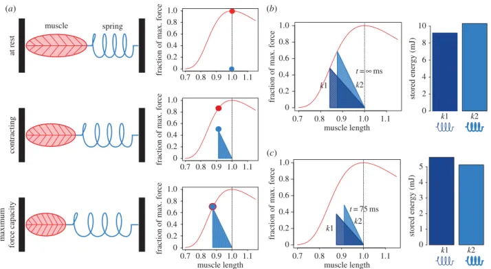
Figure 1.
During a fixed-end contraction of a muscle – spring system, the stored elastic energy depends on spring stiffness and the force the muscle generates. (
a
) At rest,
the maximum force the muscle can generate (red circle) is much higher than the force of the spring (blue circle). While the muscle contracts, maximum muscle force (red
line) decreases due to the muscle’s length– tension properties, and the spring is stretched, thereby increasing spring force. Maximum force capacity is reached when
maximum muscle force and spring force coincide. (
b
)
When given infinite time for contraction, all spring systems reach maximum force capacity and intersect with the
muscle’s length– tension curve (red line). In this example, the stored energy (area of the triangle formed) is higher in the stiffer spring system (light blue;
k
2) than the
more compliant system (dark blue;
k
1). (
c
) This relationship changes, however, when contraction duration is reduced to 75 ms, because the muscle does not reach
maximum force production in this duration owing to muscle velocity and activation effects. At this shortened duration, the less stiff spring system (
k
1) stores more
energy. The present study tests this proof-of-concept demonstration. (Online version in colour.)
rspb.r
oy
alsocietypublishing.org
Pr
oc.
R.
Soc.
B
283
:
20161561
sections, we explain how different instances of the model were used to predict force and elastic energy storage over a range of contraction scenarios.
(i) Hill-type muscle model
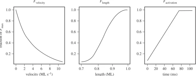
We used a Hill-type muscle model to predict muscle force as a function of three factors: muscle length, muscle velocity and muscle activation [5]. The relative contributions to muscle force by these three factors are described by equations (2.2)–(2.4):
Flength(Dxm,L0,aL,bL,s)¼eðjðððxmÞ
bLÞ1Þ=sjÞaL
, ð2:2Þ
Fvelocity(v,av,bv)¼ 1
ðv=vmaxÞ
1þ ðv=ðvmax=4ÞÞ
ð2:3Þ
and
Factivation(tcontraction,ract)¼ racttcontraction:racttcontraction ,1 1 :racttcontraction1
ð2:4Þ
wherexmis the length of the muscle with units of muscle lengths;
aL,bLandsare phenomenological parameters that were fitted to
describe the shape of the muscle’s length –tension curve; v is
muscle shortening velocity (Dxm/Dt);vmaxis the maximum
short-ening velocity of muscle contraction; tcontractionis the time the
muscle has been contracting; and ract is the linear rate of
muscle activation. We used each of these three functions in the Hill-type muscle model to scale maximum force production; therefore, these functions were evaluated from 0 to 1 and represented the fraction of maximum force that was produced by a single component (i.e. length, velocity or activation) independent of all others (figure 2).
Each of the factors impacting muscle force production were
combined to estimate muscle force (Fmuscle) by multiplying the
results of equations (2.2) –(2.4) with each other and the maximum
tetanic force of the muscle (Fmax),
Fmuscle¼FmaxFlengthFvelocityFactivation: ð2:5Þ
In this model, maximum tetanic force was generated when each
of the constituent effects on muscle force (Flength, Fvelocity and
Factivation) equalled 1.
(ii) Hookean spring model
We represented the series elastic component of the muscle – spring model with a linear, Hookean spring. Although biological springs are not Hookean, many springs, including those of bull-frogs and grasshoppers, approximate linear behaviour over a
significant region of the force –displacement curve [10,17]. For this model, spring force was determined only by the
displace-ment through which it is stretched (Dxs) and the spring
stiffness (ksimulation):
Fspring¼ ksimulationDxs: ð2:6Þ
(iii) Static muscle – spring model
We allowed the muscle and spring models to interact by setting
two groups of variables equal:Fmuscle equalledFspring, and the
muscle shortening length change equalled the negative of spring
stretch length change (i.e.Dxm¼2Dxs; see figure 1 for schematic):
FmaxFlength(Dxm,L0,aL,bL,s)Fvelocity(v,vmax)
Factivation(tcontraction,ract)¼ ksimulationDxs: ð2:7Þ
To simplify the model, variables that described muscle proper-ties (i.e. variables that were only used to determine the shape of the Hill-type muscle components) were held constant for a given muscle. We further simplified equation (2.7) to represent a static,
steady-state solution by setting the dynamic components (Factivation
andFvelocity) to 1:
FmaxFlength(Dx,L0,aL,bL,s)¼ ksimulationDx, ð2:8Þ
withDx¼Dxm¼2Dxs.
Solving for Dx in equation (2.8) resulted in the maximum
internal stretch of that particular spring by its in-series muscle. This value was used to calculate maximum stored elastic energy in the static simulations, the case in which contraction time to store spring energy is not limited (see figure 1 for schematic).
(iv) Dynamic muscle – spring model
The dynamic muscle –spring model was identical to the static
model with one exception: we did not setFactivationandFvelocity
equal to 1 in equation (2.7). Holding all muscle properties
con-stant and considering velocity as Dxm and Dt resulted in the
dynamic model
FmaxFlength(Dx,L0,aL,bL,s)Fvelocity(Dx,Dt)
Factivation(tcontraction,ract)¼ ksimulationDxs: ð2:9Þ
Solving for Dx at each time step was complicated by the
relationship between muscle length and contraction velocity,
because Dxm affected muscle force in two ways. First, Dxm
affectedFlength directly; values of Dxm/L0smaller than 1 (as a
result of muscle shortening contraction) decreased muscle force
(figure 2). Second, for a givenDt, greater values ofDxmresulted
in greater contraction velocities. This reduced muscle force
0.8
0.6 1.0
0.2 0.4
0 4 6 8 10
velocity (ML s–1)
fraction of
Fmax
0.8
0.6 1.0
0.2 0.4
0.8
0.6 1.0
0.2 0.4
Fvelocity
0.7 0.8 0.9 1.0 length (ML)
Flength
0 20 40 60 80 100 time (ms)
Factivation
2
Figure 2.
In the Hill-type muscle model, force depends on three components: length, velocity and activation. The contributions of each component are
mathematically defined in equations (2.2) – (2.4). Each plot was generated using properties of bullfrog plantaris longus muscle.
rspb.r
oy
alsocietypublishing.org
Pr
oc.
R.
Soc.
B
283
:
20161561
Fvelocity(equation (2.3)). Given that contractions causing larger
muscle excursions Dxm increased force production by the
spring and reduced force production by the muscle (owing to both Flength and Fvelocity), the challenge was to determine, at
every time step of the simulation, which value ofDx satisfied
equation (2.9).
To satisfy all force, displacement and velocity assumptions, we
employed a numerical technique that calculatedFmuscleandFspring
for many values ofDxat each time step. Starting with the first time
step, we tested 5000 equally spacedDxm(with units of fraction of
L0) and plugged them into equation (2.9), and thereby generated
many hypothetical combinations ofFmuscleandFspring. We then
selected the value ofDxmthat resulted in the smallest difference
betweenFmuscleandFspring. We repeated this numerical technique
for all subsequent time steps until the muscle and spring reached static equilibrium (i.e. when the change in muscle length between
two time steps fell below an arbitrary value of 0.0001L0).
(b) Inputs to the muscle – spring model
Muscle parameters. Simulations of a bullfrog and grasshopper
were conducted using parameter values for components of the Hill-type model taken from previous studies (table 1) [10,14,15]. Although bullfrog muscles are pre-stretched to lengths
of 1.3L0prior to tendon loading [14], grasshopper muscles begin
close to 1.0 L0before jumping [10]. Therefore, to make results
from the bullfrog and grasshopper comparable, simulated con-tractions always started at the muscle resting length (bullfrog:
L0¼11.2 mm [15,18]; grasshopper:L0¼4 mm [10]), and all
com-puted length changes were converted to and reported as strain
(i.e. *L021). The shape of Factivation, which was not reported in
the literature, was approximated as a line with slope ract. The
slopes of ract were chosen such that maximum activation
occurred within biologically realistic muscle contraction times for both systems (within 100–300 ms). Based on published data, we estimated the duration of muscle contraction before
the onset of jumping (tcontraction) as 50 ms in the bullfrog [14]
and 300 ms in the grasshopper [10].
Spring parameters. Two values of spring stiffness were defined: (i) the actual experimentally measured spring stiffness of the
tendon/apodeme-cuticular spring (KbullfrogorKgrasshopper
depend-ing on the simulation) and (ii) the values of sprdepend-ing stiffness used in
the simulation to determine maximal energy storage (ksimulation).
We estimated Kbullfrog as 6.69 N mm21 using published data
from a fixed-end contraction [18]. The spring system in grasshop-pers was composed of two springs in series, the apodeme (arthropod tendon) and the cuticular semilunar process. We
calcu-lated Kgrasshopper as the effective spring stiffness of these two
springs (15.37 N mm21) by rearranging the standard equation
for two springs in series, which resulted in the equation
Kgrasshopper¼
KapodemeKSLP
KapodemeþKSLP,
ð2:10Þ
whereKapodemeandKSLPare the stiffness values of the apodeme
(31.4 N mm21) and semilunar process (30 N mm21), respectively
[10]. The values ofksimulationwere uniformly generated from 5 to
350 N *L021increments of 0.1 N *L021.
Simulation parameters. We simulated all muscle contractions with time steps of 0.001 s. The total number of steps was not determined before simulation. Instead, simulations terminated
when change in muscle length reduced to less than 0.001L021
between time steps.
Identification of kmaxE. The determination of the spring stiff-ness that permitted maximal energy storage in the static
simulations was straightforward. The value of Dx in equation
(2.8) was solved for many values of ksimulation. The stored
energy for each simulation was calculated using equation (2.1).
The value of ksimulation that resulted in the greatest stored
energy was recorded askmaxE.
ObtainingkmaxEfrom the dynamic muscle–spring model
fol-lowed a similar process; however, the data required an additional
pre-processing step. For each time step,Dx was calculated for
various values ofksimulationvia equation (2.9).
To test the effect of muscle contraction duration (tcontraction),
we ran simulations with truncated duration to exclude time
steps that were greater thantcontraction. From the truncated
data-set, kmaxE was determined using the methods above for the
static and dynamic muscle–spring models.
3. Results
(a) Static simulation
For both the bullfrog and the grasshopper, the amount of stored elastic energy was maximized for an intermediate
spring stiffness (figure 4). As ksimulation increased, stored
energy rose, levelled off and declined. In the bullfrog, the spring stiffness that permitted maximal energy storage (kmaxE; dotted lines in figure 4) equalled 20.98 N mm21, more than double the measured value of bullfrog tendon.
The amounts of energy stored withkmaxEandKbullfrog were
20.43 and 14.13 mJ, respectively (table 2). In the grasshopper,
kmaxE equalled 18.0 N mm21 and the amounts of energy
Table 1.
These muscle parameters define the length – tension and force – velocity relationships of contracting muscle of bullfrogs and grasshoppers, and were
compiled from previously published data.
parameter
value for bullfrog
value for grasshopper
definition
F
max42.7 N
c
13.1 N
amaximum tetanic force
v
max124.1 mm s
21c7.0 mm s
21amaximum contraction velocity
L
011.2 mm
c
4.0 mm
aresting length of muscle
t
contraction100 ms
c300 ms
atime until maximum
in vitro
muscle activation
a
L2.08
b
2.08
bdetermines shape of length – tension relationship
b
L2
2.89
b2
2.89
bdetermines shape of length – tension relationship
s
2
0.75
b2
0.75
bdetermines shape of length – tension relationship
mass
213.9 – 373.0 g
c1.5 – 2.0 g
arange of body mass
a
Bennet-Clark [10].
bAzizi & Roberts [14].
cSawicki
et al
. [15].
rspb.r
oy
alsocietypublishing.org
Pr
oc.
R.
Soc.
B
283
:
20161561
stored with kmaxE and Kgrasshopper were 2.24 and 2.21 mJ, respectively (table 2).
(b) Dynamic simulations
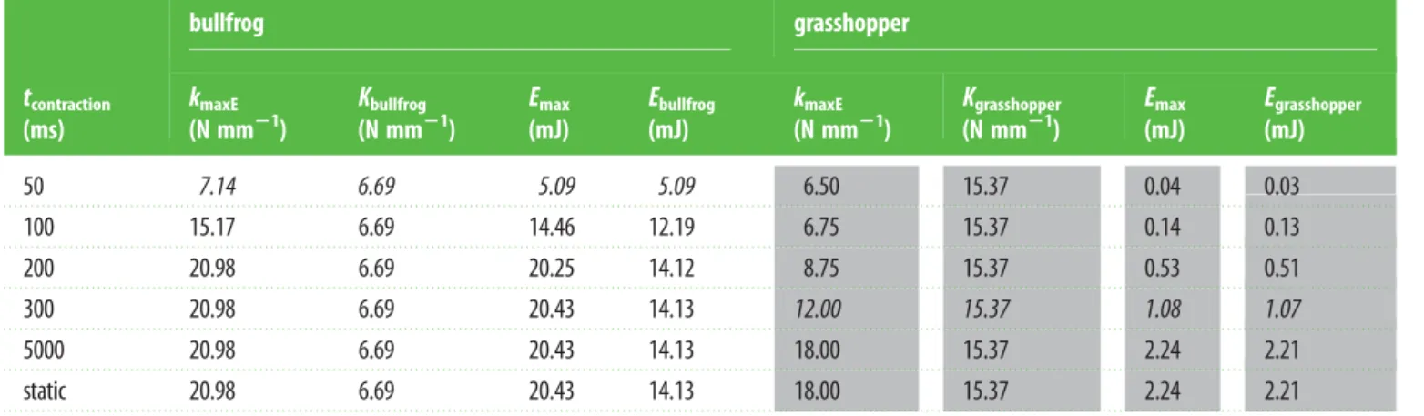
Astcontraction increased, more elastic energy was able to be stored. For example, maximal elastic energy values stored at 50, 100 and 300 ms were 5.09, 14.46 and 20.43 mJ, respect-ively, for the bullfrog and 0.03, 0.14 and 1.08 mJ for the grasshopper (table 2). In addition, all values resulting from the 5000 ms dynamic simulation matched those of the static simulation; therefore, because we reached the static steady-state solution by 5000 ms, we did not simulate muscle contraction past this time step.
Similar to the static simulation, dynamic simulations also revealed that an intermediate spring stiffness resulted in
maximal stored energy; however, the value of kmaxE was
dependent ontcontraction(figures 3 and 4). Our simulation of
the bullfrog muscle –spring system also showed that kmaxE
was higher for faster rates of contraction (figure 3); therefore, as a point of comparison between the bullfrog and the grass-hopper, unless otherwise stated, all reported results were
taken from simulations at the highestracttested, resulting in
tetanic contractions occurring in 100 ms.
In the bullfrog,kmaxEfor a realistically time-limited
contrac-tion (50 ms) was 7.14 N mm21, less than half that predicted by
the static solution (20.98 N mm21). This difference was a direct
consequence of the force–velocity property of the frog muscle.
Additionally,Kbullfrog(6.69 N mm21) was much closer tokmaxE
at 50 ms (7.14 N mm21) than to the k
maxE of the static
simulation (20.98 N mm21). Alternatively,kmaxEin the
grass-hopper for a biologically relevant contraction duration
(300 ms) was 12.0 N mm21, which matched the result
predicted by the static solution (table 2). Regardless of
simu-lation, as tduration increased, so did kmaxE until the solution
generated by the static solution was reached. This was shown by the rightward shift of the dotted line in figure 4 as time
increased. When considering the highest value of ract used
in the simulations, kmaxE did not level out until 150 ms
(figure 3). Additionally, the peak values of energy storage all occurred at the highest rates of activation (see the electronic supplementary material).
4. Discussion
By simulating the dynamic interaction between muscle and spring during a fixed-end contraction, we asked two questions: (i) Does reducing the time available for spring-loading affect which springs store the most energy? (ii) Do the values of spring stiffness in bullfrogs and grasshoppers permit maxi-mum energy storage based on their contrasting loading regimes? For both the bullfrog and the grasshopper, the time available for muscle contraction determined which spring stiff-ness permitted maximal energy storage. As time restriction increased (i.e. as less time was available for muscle contrac-tion), the values of spring stiffness that permitted maximal stored energy decreased (figure 4). Although the greatest amounts of elastic energy were predicted using the static sol-ution, this solution was not reached until 5000 ms in the grasshopper, a duration of muscle contraction that is much greater than what occurred in other experiments (table 2). Con-sequently, static simulations may be insufficient to model muscle–spring systems in some cases. The static solution,
how-ever, offered an upper bound ofkmaxEand maximum stored
energy in biological systems.
In both the bullfrog and the grasshopper, empirically measured values of spring stiffness approximately matched
kmaxEwhen taking time-limited loading into account. In the
bullfrog, dynamic simulation revealed that when the duration of muscle contraction was restricted to biologically relevant
contraction durations (50 ms),kmaxEandKbullfrogwere similar
(7.14 and 6.69 N mm21, respectively). Therefore, the
incorpor-ation of muscle dynamics into the simulincorpor-ation not only allowed the muscle–spring model to behave in a more realistic way, but it also countered the results of the static simulation and suggested that bullfrog tendons maximize energy storage at short time scales. Conversely, results from the dynamic simu-lation of the grasshopper muscle–spring system suggested that the grasshopper spring system maximized energy at rela-tively long time scales. In the case of grasshoppers, which load their springs with longer durations than bullfrogs (300 and 50 ms, respectively), the static simulation provided reasonable
estimates ofkmaxEand maximal stored energy. It is important to
note that biological springs can be tuned over evolutionary time to perform a multitude of mechanical behaviours over a wide range of loading regimes; therefore, there may be func-tional reasons that explain mismatch between our predictions of optimal stiffness and the stiffness with which organisms operate. Regardless, these two cases of dynamic fixed-end con-tractions demonstrate that muscle–spring system performance depends on the interaction between storage time available and muscle–spring properties.
The dynamic simulation of the bullfrog also demonstrated the importance of dynamics for all rates of muscle activation.
At the fastest muscle activations,kmaxEdid not level out until
150 ms (figure 3); therefore, bullfrog muscle–spring systems that complete energy storage within 150 ms are more sensitive to muscle dynamics than those that do not. Given that maximal in vitroactivation of bullfrog muscle is reached in 100 ms [15], this further demonstrated the importance of muscle dynamics in bullfrog spring systems.
duration of muscle contraction (ms) 100 150 200 250 300 50
0 5 10 15 20
spring constant for maximal energy storage (N mm
–1
)
fast contraction
slow contraction
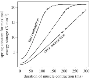
Figure 3.
Regardless of activation rate, the spring stiffness that permits
maximal energy storage (
k
maxE) is dependent on the duration of muscle
con-traction (
t
contraction). For example,
k
maxEat 300 ms (approximating the static,
steady state) is higher than
k
maxEmeasured at 50 and 100 ms. For fast
acti-vations,
k
maxEis more sensitive at smaller durations of muscle contraction,
demonstrated by the steep slope. The fast, intermediate and slow activations
reach maximum activation within 100, 200 and 300 ms, respectively. Data
shown are from the bullfrog model.
rspb.r
oy
alsocietypublishing.org
Pr
oc.
R.
Soc.
B
283
:
20161561
The results of the simulations hinted at the relationship between compliant springs and energy storage. As muscle con-traction duration decreases, the total amount of elastic energy that can be stored decreased (figure 4). Additionally, the
sensi-tivity ofkmaxEto muscle dynamics increased as the duration of
muscle contraction decreased (figure 3). Therefore, in muscle– spring systems that are time-limited, reducing spring stiffness could help maximize energy in situations in which stored energy is decreased owing to short contraction durations. In short, when muscle dynamics became important, optimal spring stiffness decreased.
Given that the results from the simulation were generated by connecting a Hill-type muscle model to a Hookean spring model, it is important to note the limitations of these constitu-ent models in the context of this study. The Hill muscle model has been shown to accurately represent general trends in the relationship between the dynamics of muscle activation and force production [19–21]. This relationship, however, was highly dependent on activation dynamics
[22,23] and may not have been accurately represented in this study. Instead of focusing on the intricacies of neuronal firing, we simplified muscle activation as a linear ramp to test, in general, whether muscle activation rate affected time-limited energy storage. To that effect, the model demon-strated that muscle dynamics played a part in determining which spring stiffness permitted maximal energy storage.
Additionally, our muscle–spring model does not
incorporate inertial effects of muscle mass on contraction vel-ocity [24] or activation-dependent shifts in the muscle length– tension relationship [25]. As a first approximation of how these effects may affect our interpretation of our results, we conducted a sensitivity analysis of our model by
perturb-ing each parameter +20% (including Vmax and starting
length to represent inertial and activation effects,
respect-ively). We found that while increases in Vmax led to
increases inEmax, predictions ofkmaxEwere relatively
insensi-tive (see the electronic supplementary material); therefore, inertial effects had little effect on our predictions of optimal 5
0 10 15 20 25
ksimulation (N mm–1)
5
0 10 15 20 25
ksimulation (N mm–1)
5
0 10 15 20 25
ksimulation (N mm–1)
5
0 10 15 20 25
ksimulation (N mm–1)
5 14
10
6
2
20
15
10
5
20
15
10
5 4
3
2 stored energy (mJ)
stored energy (mJ) stored energy (mJ) stored energy (mJ)
50 ms 100 ms 300 ms static
0.026 0.030 0.034
stored energy (mJ) stored energy (mJ) 0.10 0.12 0.14
stored energy (mJ)
0.5 0.7 0.9 1.1
ksimulation (N mm–1) k
simulation (N mm–1) ksimulation (N mm–1) ksimulation (N mm–1)
40 30
0 10 20 0 10 20 30 40 0 10 20 30 40 0 10 20 30 40
stored energy (mJ)
0.5 1.0 1.5 2.0
Kgrasshopper Kgrasshopper Kgrasshopper Kgrasshopper Kbullfrog Kbullfrog Kbullfrog Kbullfrog
Figure 4.
The duration of muscle contraction (
t
contraction) determines whether the spring stiffness of bullfrog tendon (
K
bullfrog, indicated by arrow) permits maximal
energy storage. For example, in the static simulation,
K
bullfrogdoes not coincide with the peak of the curve (indicated by dotted line). Results from the static
simulation suggest that
K
bullfrogdoes not permit maximal energy storage. Conversely, during time-limited muscle contractions (50 ms),
K
bullfrogis closer to the
peak of the curve. The leftward shift of the peak as
t
contractionis reduced suggests that muscle – spring dynamics become increasingly important with shorter
dur-ations of muscle contraction. Conversely, in grasshoppers, the static solution is a close approximation of the results from the biologically relevant loading time
(300 ms). Results from simulations that occur at biologically relevant loading times are boxed. Note that the scale of the
y
-axis is different in each panel.
Table 2.
As the duration of muscle contraction approaches biologically relevant durations (italicized values),
k
maxEapproaches the measured spring stiffness
(
K
bullfrogand
K
grasshopper). Static simulations accurately model systems that exhibit relatively long loading times, such as the grasshopper (grey-shaded values).
Dynamic simulations are necessary for systems that exhibit time-limited contraction, such as the bullfrog (unshaded).
t
contraction(ms)
bullfrog
grasshopper
k
maxE(N mm
21)
K
bullfrog(N mm
21)
E
max(mJ)
E
bullfrog(mJ)
k
maxE(N mm
21)
K
grasshopper(N mm
21)
E
max(mJ)
E
grasshopper(mJ)
50
7.14
6.69
5.09
5.09
6.50
15.37
0.04
0.03
100
15.17
6.69
14.46
12.19
6.75
15.37
0.14
0.13
200
20.98
6.69
20.25
14.12
8.75
15.37
0.53
0.51
300
20.98
6.69
20.43
14.13
12.00
15.37
1.08
1.07
5000
20.98
6.69
20.43
14.13
18.00
15.37
2.24
2.21
static
20.98
6.69
20.43
14.13
18.00
15.37
2.24
2.21
rspb.r
oy
alsocietypublishing.org
Pr
oc.
R.
Soc.
B
283
:
20161561
spring stiffness. Conversely, the most sensitive parameter in the simulation was the starting length of the muscle. Our model predicted peak energy storage when muscles began activating on the descending limb of the length –tension
curve (approx. 1.1 L0, regardless of study system; see
elec-tronic supplementary material). Consequently, starting muscles at these lengths required decreases in spring stiffness
(243.75% and 250.0% in bullfrogs and grasshoppers,
respectively). These analyses indicate that because kmaxE is
highly dependent on the muscle length–tension curve, activation-dependent effects probably affect the relationship between spring mechanics and muscle physiology. In order to accurately model this in our simulation, however, more information is needed about how muscle activation affects the shape of the length–tension curve in regions that span the full excursion that muscles experience during fixed-end contractions. Data regarding activation-dependent length – tension curves should be incorporated in future simulations as they become available.
The results assumed that muscle contracts at rates such that maximal activation occurs within 100 ms. In reality, different jumps from the same animal could vary in muscle activation rate, thereby affecting the amount of spring stretch. The simulations show that bullfrog muscles that took longer than 100 ms to reach maximal activation stored less elastic
energy forkmaxE(figure 3). Because the simulations were
sen-sitive to variation in muscle activation rate, reported values of
EmaxandkmaxEshould not be interpreted as exact predictions
of optimal bullfrog performance. Nonetheless, these values do provide a qualitative view of how muscle and spring parameters interact during time-limited energy storage.
Another simplification of the model involved the use of a linear spring. Most biological structures, including bullfrog tendons, exhibit a toe region of low spring stiffness early in the force–displacement curve followed by a linear region of higher spring stiffness. Many studies remedy this by measuring spring stiffness in the linear region of the force–displacement curve. In addition, it is important to note that the simulation only predicted the amount of energy stored, but other factors such as mass, material properties and morphological lever systems directly impact the unloading of energy [26,27].
Our dynamic simulations revealed a phenomenon that potentially affects all spring systems that are transiently loaded by muscle. That is, muscles that cannot develop iso-metric force because of time restriction can achieve significant amounts of elastic energy storage when coupled with springs of lower stiffness than would be predicted in the static case. For example, because bullfrogs lack morphological latches, they are not able to load their springs with peak isometric force. Instead, the bullfrog uses a dynamic catch mechanism, which temporarily resists force via inertial loads and mechan-ical advantage about moving joints [28]. The dynamic catch is able to resist some muscle contraction to permit spring-loading, but not long enough for isometric contractions to develop. With the exception of salamanders and chameleons, which probably contain anatomical latches [29,30], and toads, which have been hypothesized to store energy via co-contraction of antagonistic muscle [31], it is likely that vertebrates are inherently subject to time-limited energy storage, and potentially benefit from springs less stiff than expected.
Conversely, we predict that some invertebrate systems with anatomical latches may operate with relatively higher spring stiffness that can permit maximal energy storage over long
storage times. Systems that have anatomical latches, and those that use rigid connections of body parts to resist muscle contrac-tion, can develop isometric contractions during spring-loading.
For example, snapping shrimp (Alpheus californiensis), trap-jaw
ants and froghoppers (Philaenus spumarius) contain body parts
that lock together to form a latch and have springs that are con-nected to slow, forceful muscles that contract isometrically for up to several seconds [2–4,32–34]. Given the amount of power amplification observed in these systems, it is likely that these muscle–spring systems are operating with spring stiffness that permits maximal energy storage.
In some systems, the determination of an optimal spring stiffness can be complicated by an active latch, in which an antagonist muscle contracts to keep a system latched. Active latches may permit variation in the amount of stored energy prior to movement [35–37]. For example, the bush cricket can use changes in both joint angle and activation of the latching muscle to determine how much force holds the latch in place [36]. Meanwhile, a larger muscle can load the spring until it exceeds the force of the latch, thereby initiating movement. Given that the bush cricket can control the amount of energy stored, it is possible that it operates with a spring stiffness that results in the most stored energy for a wide range of situations. Although this idea is speculative, this study provides the tools necessary to test this hypothesis in other active latch systems in future work.
5. Conclusion
When testing for maximal energy storage, it is important to consider the dynamic interaction of muscle and spring. Our simulations revealed that within the realm of biologically rel-evant time scales, the more time available for loading by muscle, the stiffer the series spring required for maximum elas-tic energy storage. Muscles that load in-series springs over shorter time scales benefit from less stiff springs. At short time scales, muscle force is small owing to low activation and high velocity, and less stiff springs allow the spring to stretch more for a given amount of force. Thus, it is necessary to deter-mine the effect, if any, of muscle dynamics on energy storage before concluding whether or not muscle–spring systems maximize energy storage.
Ethics. All animal information was based on previously published datasets.
Data accessibility.All R code used for simulations can be found at http:// dx.doi.org/10.17605/OSF.IO/Z385A. Data generated from the simu-lation have been uploaded to Dryad (http://dx.doi.org/10.5061/ dryad.089cr).
Authors’ contributions.M.V.R. implemented the mathematical model, ran all dynamic simulations, analysed the data and prepared the manu-script, G.P.S. conceived the original idea of the static model and guided the study to include grasshoppers, S.N.P. helped prepare the manuscript and identified key points/questions of the study, G.S.S. helped develop the dynamic model and simulations, provided data from bullfrogs, offered insight on data analysis/interpretation and helped edit the manuscript.
Competing interests.We have no competing interests.
Funding.This research was supported by grants awarded to M.V.R. (DOE FG02-97ER25308) and S.N.P. (NSF IOS-1439850).
Acknowledgements.The authors thank W. M. Kier, K. K. Smith, D. M. Boyer and E. Azizi for providing feedback on the manuscript. We also appreciate comments and contributions from P. Green, P. S. L. Anderson, K. Kagaya, R. Crane. We thank the DOE CSGF for training provided for high-speed computing.
rspb.r
oy
alsocietypublishing.org
Pr
oc.
R.
Soc.
B
283
:
20161561
References
1. Hill AV. 1938 The heat of shortening and the dynamic constants of muscle.Proc. R. Soc. Lond. B. 126, 136 – 195. (doi:10.1098/rspb.1938.0050) 2. Ritzmann R. 1973 Snapping behavior of the shrimp
Alpheus californiensis.Science181, 459 – 460. (doi:10.1126/science.181.4098.459)
3. Ritzmann R. 1974 Mechanisms for the snapping behavior of two alpheid shrimp,Alpheus californiensisandAlpheus heterochelis.J. Comp. Physiol.95, 217 – 236. (doi:10.1007/BF00625445) 4. Burrows M. 2007 Neural control and coordination of
jumping in froghopper insects.J. Neurophysiol.97, 320 – 330. (doi:10.1152/jn.00719.2006)
5. Zajac FE. 1989 Muscle and tendon: properties, models, scaling, and application to biomechanics and motor control.Crit. Rev. Biomed. Eng.17, 359 – 411.
6. Zajac FE, Gordon ME. 1989 Determining muscle’s force and action in multi-articular movement.Exerc. Sport Sci. Rev.17, 187 – 230.
7. Wilson AM, Watson JC, Lichtwark GA. 2003 Biomechanics: a catapult action for rapid limb protraction.Nature.421, 35 – 36. (doi:10.1038/ 421035a)
8. Patek S, Rosario MV, Taylor J. 2013 Comparative spring mechanics in mantis shrimp.J. Exp. Biol. 216, 1317 – 1329. (doi:10.1242/jeb.078998) 9. Rosario MV, Patek SN. 2015 Multilevel analysis of elastic
morphology: the mantis shrimp’s spring.J. Morphol. 276, 1123–1135. (doi:10.1002/jmor.20398) 10. Bennet-Clark HC. 1975 The energetics of the jump
of the locustSchistocerca gregaria.J. Exp. Biol.63, 53 – 83.
11. Marsh RL, John-Alder HB. 1994 Jumping performance of hylid frogs measured with high-speed cine film.J. Exp. Biol.188, 131 – 141. 12. Peplowski MM, Marsh RL. 1997 Work and power
output in the hindlimb muscles of Cuban tree frogs
Osteopilus septentrionalisduring jumping.J. Exp. Biol.200, 2861 – 2870.
13. Roberts TJ, Marsh RL. 2003 Probing the limits to muscle-powered accelerations: lessons from jumping bullfrogs.J. Exp. Biol.206, 2567 – 2580. (doi:10. 1242/jeb.00452)
14. Azizi E, Roberts TJ. 2010 Muscle performance during frog jumping: influence of elasticity on muscle
operating lengths.Proc. R. Soc. B277, 1523 – 1530. (doi:10.1098/rspb.2009.2051)
15. Sawicki GS, Sheppard P, Roberts TJ. 2015 Power amplification in an isolated muscle-tendon is load dependent.J. Exp. Biol.218, 3700 – 3709. (doi:10. 1242/jeb.126235)
16. Winters J. 1990 Hill-based muscle models: a systems engineering perspective. InMultiple muscle systems: biomechanics and movement organization
(eds JM Winters, SL-Y Woo), pp. 69 – 93. New York, NY: Springer.
17. Hollinger JO. 2011An introduction to biomaterials. Boca Raton, FL: CRC/Taylor & Francis.
18. Sawicki GS, Robertson BD, Azizi E, Roberts TJ. 2015 Timing matters: tuning the mechanics of a muscle – tendon unit by adjusting stimulation phase during cyclic contractions.J. Exp. Biol.218, 3150 – 3159. (doi:10.1242/jeb.121673)
19. Cofer D, Cymbalyuk G, Reid J, Zhu Y, Heitler WJ, Edwards DH. 2010 AnimatLab: a 3D graphics environment for neuromechanical simulations.
J. Neurosci. Methods187, 280 – 288. (doi:10.1016/j. jneumeth.2010.01.005)
20. Winters TM, Takahashi M, Lieber RL, Ward SR. 2011 Whole muscle length – tension relationships are accurately modeled as scaled sarcomeres in rabbit hindlimb muscles.J. Biomech.44, 109 – 115. (doi:10.1016/j.jbiomech.2010.08.033)
21. Richards CT, Sawicki GS. 2012 Elastic recoil can either amplify or attenuate muscle-tendon power, depending on inertial vs. fluid dynamic loading.J. Theor. Biol.313, 68– 78. (doi:10.1016/j.jtbi.2012.07.033)
22. Josephson RK. 1985 Mechanical power output from striated muscle during cyclic contraction.J. Exp. Biol. 114, 493 – 512.
23. Stevens ED. 1996 The pattern of stimulation influences the amount of oscillatory work done by frog muscle.J. Physiol.494, 279 – 285. (doi:10. 1113/jphysiol.1996.sp021490)
24. Ross SA, Wakeling JM. 2016 Muscle shortening velocity depends on tissue inertia and level of activation during submaximal contractions.
Biol. Lett.12, 20151041. (doi:10.1098/rsbl. 2015.1041)
25. Holt NC, Azizi E. 2016 The effect of activation level on muscle function during locomotion: are optimal
lengths and velocities always used?Proc. R. Soc. B
283, 20152832. (doi:10.1098/rspb.2015.2832) 26. McHenry MJ, Claverie T, Rosario MV, Patek SN. 2012
Gearing for speed slows the predatory strike of a mantis shrimp.J. Exp. Biol.215, 1231 – 1245. (doi:10.1242/jeb.061465)
27. Anderson PSL, Claverie T, Patek SN. 2014 Levers and linkages: Mechanical trade-offs in a power-amplified system.Evolution68, 1919 – 1933. (doi:10.1111/evo.12407)
28. Astley HC, Roberts TJ. 2014 The mechanics of elastic loading and recoil in anuran jumping.J. Exp. Biol. 217, 4372 – 4378. (doi:10.1242/jeb.110296) 29. de Groot JH, van Leeuwen JL. 2004 Evidence for an
elastic projection mechanism in the chameleon tongue.Proc. R. Soc. Lond. B.271, 761 – 770. (doi:10.1098/rspb.2003.2637)
30. Deban SM, O’Reilly JC, Dicke U, van Leeuwen JL. 2007 Extremely high-power tongue projection in plethodontid salamanders.J. Exp. Biol.210, 655 – 667. (doi:10.1242/jeb.02664)
31. Nishikawa KC. 1999 Neuromuscular control of prey capture in frogs.Phil. Trans. R. Soc. Lond. B354, 941 – 954. (doi:10.1098/rstb.1999.0445)
32. Gronenberg W, Tautz J, Holldobler B. 1993 Fast trap jaws and giant neurons in the antOdontomachus.
Science262, 561 – 563. (doi:10.1126/science.262. 5133.561)
33. Patek SN, Baio J, Fisher B, Suarez A. 2006 Multifunctionality and mechanical origins: ballistic jaw propulsion in trap-jaw ants.Proc. Natl Acad. Sci. USA103, 12 787 – 12 792. (doi:10.1073/pnas. 0604290103)
34. Patek SN, Dudek DM, Rosario MV. 2011 From bouncy legs to poisoned arrows: elastic movements in invertebrates.J. Exp. Biol.214, 1973 – 1980. (doi:10.1242/jeb.038596)
35. Burrows M, Morris G. 2001 The kinematics and neural control of high-speed kicking movements in the locust.J. Exp. Biol.204, 3471 – 3481. 36. Burrows M. 2003 Jumping and kicking in bush
crickets.J. Exp. Biol.206, 1035 – 1049. (doi:10. 1242/jeb.00214)
37. Kagaya K, Patek SN. 2016 Motor control of ultrafast, ballistic movements.J. Exp. Biol.219, 319 – 333. (doi:10.1242/jeb.130518)