The Effect of Franchising on Store Performance and Consumer Utility
Jeffrey Ackermann
A dissertation submitted to the faculty of the University of North Carolina at Chapel Hill in partial fulfillment of the requirements for the degree of Doctor of Philosophy in
the Department of Economics
Chapel Hill 2017
c
2017
ABSTRACT
JEFFREY ACKERMANN: The Effect of Franchising on Store Performance and Consumer Utility
(Under the direction of Brian McManus)
I estimate the effect that franchising a store has on its performance. There is a substantial literature predicting that a franchisee-owned store will generate higher profits than a franchisor-owned store, all else equal. However, attempts to estimate the effect of franchising on store performance are hampered by an important selection issue: the franchisor may choose to assign the least desirable locations to franchisees. I overcome this issue by using a 2007 corporate sale that resulted in all franchisor-owned Applebee’s stores in Texas being sold to franchisees as a source of exogenous variation. While I do not observe store profits, Texas makes store-level alcohol sales data available for all bars and restaurants that have a liquor license; I use alcohol revenues as a proxy for store performance.
ACKNOWLEDGMENTS
I would like to first thank my dissertation advisor, Brian McManus, for his encour-agement and mentoring. I would next like to thank the other members of my dissertation committee: Gary Biglaiser, Luca Flabbi, Helen Tauchen, and Jonathan Williams for the valuable feedback that they provided me. I would also like to thank Tiago Pires. He was an outstanding economist, an incredible friend to everyone in our department, and one of the most joyful people you could ever meet. I am grateful to the attendees of the applied microeconomics workshop at UNC, both the faculty and my fellow graduate students. Their questions both guided my research and prepared me to present my work to an outside audience. I am especially appreciative of Forrest Spence and Brad Shrago for their insights.
Relating to teaching, I first would like to thank Helen Tauchen for allowing me to teach and for working with my schedule. I am thankful to Jeremy Petranka for his guidance and confidence in me. I would like to thank the economics department administrative staff and the individuals who have served as my teaching assistants; they all made my teaching assignments immeasurably easier.
TABLE OF CONTENTS
List of Tables . . . viii
List of Figures . . . x
1 Background . . . 1
1.1 Review of Literature . . . 2
1.1.1 Interfirm Relationships and Moral Hazard . . . 2
1.1.2 Franchising . . . 5
1.1.3 Models of Spatial Competition . . . 15
1.2 Institutional Details . . . 16
1.2.1 Sale to IHOP . . . 18
1.3 Motivational Model of Ownership Selection . . . 19
1.4 Data . . . 22
1.5 Additional Data Discussion . . . 26
1.6 Franchisor’s Ownership Selection Process . . . 27
2 Reduced Form Analysis . . . 51
2.1 Empirical Analysis of the Franchisor’s Ownership Decision . . . 51
2.2 Initial Estimates of the Effect of Franchising . . . 53
2.3 Comparison with Buffalo Wild Wings . . . 58
2.4 Conclusion . . . 61
3 Structural Model . . . 80
3.2 Econometric Analysis . . . 87
3.3 Results . . . 88
3.4 Simulations . . . 93
3.5 Conclusion . . . 97
A Estimation of Unobservables in Selection Model . . . 103
B Data Appendix . . . 104
LIST OF TABLES
1.1 Franchise Fees for Various Casual Dining Chains . . . 32
1.2 Sample of Menu Items and Prices . . . 33
1.3 Summary Statistics for the First Quarter of 2013 . . . 34
1.4 County Level Statistics for 2013 . . . 35
1.5 Ownership of New Stores and Nearest Existing Stores . . . 36
1.6 County-Level Averages by Applebee’s Ownership Type, Q4 2006 . . . 37
1.7 Summary Statistics for Applebee’s Alcohol Revenues by Ownership Type, Q4 2006 . . . 38
1.8 Summary Statistics for Applebee’s Alcohol Revenue by Ownership Type, Q4 2006 and Q4 2013 . . . 38
1.9 Average Revenue by Quarter . . . 39
2.1 Logit Model Predicting if a Store Will be Franchised . . . 63
2.2 Logit Model Predicting if a Store Will be Franchised - Only Stores Open in Q2 2001 Included . . . 64
2.3 Logit Model Predicting the Initial Franchise Status of Applebee’s Stores in Each County . . . 65
2.4 Estimated Effect of Franchising: Fixed Effects Model . . . 66
2.5 Logit Model Predicting if a Buffalo Wild Wings Store Will be Franchised 67 2.6 Impact of Demographics on Buffalo Wild Wings Store Revenue . . . 68
2.7 Using Nearby Applebee’s Store Ownership to Predict Buffalo Wild Wings Store Revenue . . . 69
2.9 Prediction of Buffalo Wild Wings Store Revenue - 2009 and Later . . . . 71
2.10 Estimated Effect of Franchising: Comparison of Time Trends . . . 72
2.11 Estimated Effect of Franchising: Alternative Specifications . . . 73
3.1 Parameter Estimates . . . 99
3.2 Impact of Franchising - Utility Comparisons and Simulation Results . . . 101
LIST OF FIGURES
1.1 Number of Applebee’s Stores by Year . . . 40
1.2 Number of Stores for Each Chain . . . 40
1.3 Average Q1 Alcohol Revenue per Store . . . 41
1.4 Income Quartile Cutoffs for Q1 of Each Year . . . 41
1.5 Statewide Alcohol Revenues . . . 42
1.6 Statewide Income and Alcohol Spending . . . 43
1.7 Histogram of Alcohol Sales for Q1 2013 . . . 44
1.8 Histogram of Logged Alcohol Sales for Q1 2013 . . . 44
1.9 2006 Map of Chain Stores . . . 45
1.10 Locations of Company Owned Applebee’s . . . 46
1.11 Locations of Franchised Applebee’s . . . 47
1.12 Histogram of Store Revenues by Ownership Type for Q4 2006 . . . 48
1.13 Histograms of Store Revenue for Q4 2006 and Q4 2013 . . . 49
1.14 Average Yearly Sales by Ownership Type . . . 50
2.1 Fixed Effects Regression Estimate of Yearly Control Variables . . . 74
2.2 Histogram of Estimated Franchise Effects by Store . . . 74
2.3 Relationship Between Estimated Store-Level Franchise Effect and 2006 Revenue . . . 75
2.4 Locations of Company Owned Buffalo Wild Wings Stores . . . 76
2.5 Locations of Franchised Buffalo Wild Wings Stores . . . 77
CHAPTER 1
BACKGROUND
My dissertation work examines the impact of franchising on firms and consumers. The research is unique because it identifies a selection problem and then uses a unique identification strategy to solve the problem and provide an estimate of the effect of franchising on firm performance. While a substantial body of research has been done regarding the reasons that firms choose to franchise some or all of their stores, little work has been done on how franchising affects a store’s performance. Attempts to estimate the effect of franchising on store performance have been hampered by an important selection issue: the franchisor selects the ownership of each store and can therefore choose the ownership configuration that maximizes franchisor profits. This may lead to the franchisor owning stores in the most desirable locations while franchisees are assigned the less lucrative locations. Thus, it is important to determine if differences in store performance between company-owned and franchisee-owned stores are due to differences in ownership or differences in location quality. I use a novel data source and a unique source of identification to identify the effect of franchising on store performance.
chapter ends with a discussion of the data used in this dissertation: restaurant-level alcohol tax revenues in the state of Texas.
In the second chapter, I first present evidence that, prior to the corporate sale, both observable and unobservable location level factors were important in Applebee’s decision to own or franchise a store. I then use a linear model with store level fixed effects to estimate the effect of franchising on store performance. I find that franchising a store has a positive impact on revenue, and I find that failing to account for unobservable differences in location quality would have resulted in the effect of franchising being underestimated. In the third chapter, I create a structural demand model which uses consumer and store locations to predict alcohol sales for all bars and restaurants in Texas with a liquor license over a ten year period. I find that franchising an Applebee’s restaurant increases its revenue by about 7 percent and provides substantial utility gains to consumers.
1.1 Review of Literature
Interfirm relationships account for approximately half of all economic activity in the United States and are the subject of a substantial amount of theoretical and empirical work. Included in this research is an extensive literature discussing the tradeoffs between vertical integration and vertical separation. In this section, I first provide an overview of literature that discusses the role moral hazard plays in interfirm relationships. I then provide a longer discussion of literature that specifically discusses franchising as an organizational form. Lastly, I discuss research that uses empirical models of spatial competition.
1.1.1 Interfirm Relationships and Moral Hazard
Moral hazard has frequently been used to help explain the nature of interfirm rela-tionships. Here I discuss research on interfirm relationships that is especially relevant for my work.
firms will choose to use an outside firm, rather than employees, to sell their products.1
Grossman and Hart (1986) generate a theoretical model that considers both principal (upstream) and agent (downstream) moral hazard when assessing the tradeoffs associated with vertical integration.
Holmstrom and Milgrom (1994) create a model that looks at various methods, which the authors list as “high-performance incentives, worker ownership of assets, and worker freedom from direct controls”, for motivating workers. The authors are especially in-terested in why many relationships between firms and employees or contractors include aspects of all three methods. This is important in the context of franchising, because these methods are all exhibited in the franchising relationship. The authors find that each method can be successfully used to mitigate worker moral hazard, and that the methods are often compliments.
Slade (1998) examines a vertical relationship known as “traditional franchising.” Tra-ditional franchising occurs when a franchisor manufactures a product and sells it to the franchisee, who resells the product to customers. Traditional franchising is substantially different from business format franchising, which is the subject of my dissertation. Her model indicates that, when it is difficult to monitor franchisee effort or when high retail prices charged by one franchisee may hurt the brand’s reputation, it is advantageous for the franchisor to choose the price charged by franchisees. She then tests these predictions using an empirical analysis of the relationship between oil companies (franchisors) and affiliated service stations (franchisees) in Vancouver.2 Using price and sales data, she
finds evidence supporting her predictions. She also finds that, when pricing decisions are delegated to the retailer, prices tend to be higher.
1Lafontaine (1992), Sen (1993), and Scott (1995) each use a similar empirical analysis to investigate
the motivations for franchising.
2Fuel retailing is one industry in which traditional franchising is very common. Other industries
Several papers look at the economics of sharecropping. Sharecropping has many similarities to franchising. Like franchising, a downstream firm (the tenant farmer) pays the upstream firm (the land owner) for the rights to use the assets of the upstream firm, and a portion of the farmer’s payment is a form of revenue sharing. Stiglitz (1974) was among the first to analyze two possible reasons for the sharecropping relationship to exist. The first is risk sharing. He notes that farming is an inherently risky venture and contrasts two organizational forms that would result in one party assuming all of the risk: in one scenario, the farmer would be paid a fixed salary, leading to all risk being borne by the franchisor, while in another scenario, the farmer would rent the land at a fixed fee from the landowner, leading to all risk being borne by the farmer. Sharecropping, on the other hand, allows both parties to assume some risk, because franchisee payments are lower during low-yield years and greater during high-yield years. The second reason he gives for the existence of sharecropping is monitoring difficulties; specifically, if the landowner is unable to monitor farmer effort, a purely wage-based compensation method will result in shirking by the farmer. Stiglitz also explores the interactions between risk aversion and monitoring difficulties. While the optimal contract from a monitoring difficulty perspective is one in which the farmer rents the land at a fixed fee (and, therefore, bears the full cost of shirking), risk averse farmers will tend to have some revenue sharing in their contracts.
1.1.2 Franchising
I now look closer at one specific type of interfirm relationship: franchising. Franchising is an organizational form in which a franchisor creates a product, business plan, and trademarks and then sells the right to open a branded store to a franchisee. The contract typically contains both a fixed fee and a variable component that depends on store performance. Thus, the franchisor acts as the upstream firm while the franchisee acts as the downstream firm.
Mathewson and Winter (1985) develop some theoretical foundations for the economics of franchise contracts. They find that the potential for franchisee free riding is a necessary condition for franchising to be an optimal strategy. They also predict that franchisors will execute some degree of control over franchisees, such as imposing quality standards and business practice standards.
Brickley and Dark (1987) empirically examine chains that have both franchisor-owned and franchisee-owned stores. They find that stores in locations with high monitoring costs are more likely to be franchised; this is evidence that franchising is used to solve a moral hazard problem. They also find that chains where stores are likely to serve the same customers repeatedly tend to franchise a larger share of their stores; this supports the hypothesis that franchisees free-riding on the franchisor’s brand is an important concern. Specifically, a franchisee who rarely serves repeat customers will be tempted to serve a low-quality product, because the negative impact of the diminished brand reputation will be borne largely by other stores. Interestingly, while a common prediction in theoretical literature is that a store located at a highway exit will be less likely to serve repeat customers and therefore less likely to be franchised,3 Brickley and Dark find no such
relationship.4 They theorize that a store’s proximity to a highway exit is not a good
predictor of its likelihood of serving repeat customers.
Minkler (1990) introduces what he describes as a “search cost” reason for franchising. He explains that if franchisees “possess superior knowledge about local markets, they can more cheaply search for the best inputs, production processes, and marketing strategies...” I refer to this as the “local expert” theory throughout my dissertation. He then tests this hypothesis using data on locations, opening dates, and franchise status for Taco Bell stores located in California and Nevada. He finds some limited evidence supporting his theory.
3Rubin (1978) and Mathewson and Winter (1985) both make this prediction.
Lafontaine (1992) uses data on 548 franchisors with 150,000 total affiliated stores to test various theories related to franchising. She finds that chains that operate in more states (which she uses as a proxy for geographic dispersion) and chains that require more discretion on the part of the store’s manager are more likely to use franchising; this supports the hypothesis that monitoring difficulties and franchisee moral hazard are important considerations for a franchisor. She also finds that when franchisor inputs are important to store success, royalty rates are higher and more stores are company-owned. Both factors increase the franchisor’s incentive to maximize systemwide sales; thus, the results support the hypothesis that franchisor moral hazard is a significant determinant of franchising behavior. Lafontaine also observes that, for a given franchisor, each franchisee has the same fee structure. Sen (1993) uses a data set similar to that of Lafontaine and conducts similar analyses. Like Lafontaine, he finds evidence that moral hazard for both the franchisee and franchisor plays an important role in the franchising relationship. He also finds evidence that the startup investment required for a store is positively correlated with the fixed franchise fee and that a franchisor’s brand name recognition is positively correlated with its royalty rate. He finds no evidence that franchisee risk aversion is an important factor in the franchising relationship. Lafontaine and Sen both find that capital market imperfections are not an important predictor of franchising behavior.
Kaufmann and Lafontaine (1994) seek to explain why anecdotal evidence suggests that McDonald’s franchisees frequently earn positive rents, even though basic franchising theory predicts that a franchisor can design franchise fees such that the ex ante expected value of store profits go to the franchisor.5 The authors first use financial data to confirm
that franchisees do, in fact, earn positive ex ante rents. They then offer predictions of why McDonald’s allows its franchisees to earn positive economic profits. They note that McDonald’s has a strong preference for franchisees who do not hold another job and are
5The authors distinguish between ex ante and ex post rents. Specifically, they explain that ex post
closely involved in the day-to-day operations of the store, as opposed to investor groups who may take a more hands-off approach to franchise ownership. The authors theorize that this leads to franchisees with lower wealth levels and less liquidity, and that these liquidity constraints prevent McDonald’s from charging a higher initial franchise fee.
Mathewson and Winter (1994) consider the choice made by franchisors of whether to grant exclusive territories to franchisees. They construct a theoretical model which indicates that granting exclusivity to franchisees is profit maximizing when franchisee inputs are especially important to store success. This is because exclusive territories encourage franchisee investments by ensuring that the franchisee’s future profits will not be harmed by the opening of a nearby store affiliated with the same chain. They find empirical evidence that chains whose franchisees are entrusted with more decisions (as measured by the franchisees’ discretion over advertising and prices) are more likely to grant exclusive territories, supporting their hypothesis.
Schmidt (1994) uses a linear city framework to model competition between fran-chisees affiliated with the same franchisor. He finds that, in the absence of a royalty rate, competition between franchisees will result in prices that are below the price that would maximize system-wide profits. A positive royalty rate serves to increase prices to the optimal level by increasing marginal costs for the franchisees. This result is some-what counterintuitive, because royalty rates are typically thought to result in inefficient outcomes due to the fact that the marginal cost faced by the franchisee is not the true marginal cost of production and, as a result, prices are above what would be charged by a profit-maximizing vertically integrated firm. He uses the empirical results of Lafontaine (1992) and Sen (1993), which find that franchisors with more outlets (which he considers a proxy for the degree of intra-franchise competition) tend to charge higher royalty rates, as evidence supporting his theory.
opportunis-tic behavior by a franchisor. For example, a franchisor could fail to make expenditures that are necessary to maintain brand reputation. He hypothesizes that franchisors use franchisor-owned stores to incentivize themselves to maintain the brand’s reputation, thus encouraging potential franchisees to trust the franchisor’s commitment to maintain-ing brand reputation. Scott then conducts an empirical analysis similar to that used by Lafontaine (1992). He uses a different data set and different proxies from Lafontaine for the importance of franchisor effort, but obtains similar results: when franchisor effort is more important, chains tend to have a higher share of franchisor-owned stores.
Bhattacharyya and Lafontaine (1995) investigate a contracting feature common in franchising: the tendency of revenue-sharing contracts to use simple, linear rules which are not customized for each individual contract.6 They develop a model that looks at
the optimal way to write a revenue sharing or profit sharing contract when both parties are tempted to exert sub-optimal effort (double-sided moral hazard). They first find that, with some general assumptions, it can be shown that the optimal revenue sharing rule can be implemented with a linear contract. They also find that, in many cases, the optimal royalty rate does not depend on market size or franchisee characteristics. However, they do not attempt to explain why the fixed franchise fee tends to be the same for all franchisees.
Lutz (1995) focuses on asset ownership in franchising, specifically that franchisees own many local assets, but franchisors own trademarks and other assets. She asserts that, while franchising is considered to be used primarily to mitigate moral hazard issues by properly incentivizing the manager, a properly designed incentive plan could accomplish the same goals without franchising; specifically, the manager of a company-owned store could have her pay more closely tied to the store’s performance. She then suggests that asset ownership is a crucial component of franchising and that, because both the
6In the case of franchising, this means that franchisees pay a fixed share of their revenue to the
franchisee and franchisor own brand-specific assets, both are motivated to maximize chain profits. Furthermore, she finds that franchising may be a profit-maximizing arrangement even if employee managers are as productive as franchisees.
Lafontaine (1995) and Graddy (1997) both compare the prices charged at company-owned and franchisee-company-owned fast food restaurants. Both find that franchisee-company-owned es-tablishments charge higher prices. Lafontaine gives two possible reasons for this finding. The first is a form of double marginalization in which the royalty rate acts as a tax on the franchisee. The second is the possibility that a low price at one store can in-crease system-wide demand by building a reputation of being a low-price chain. Because the franchisor’s profits are more tied to system-wide sales than a franchisee’s are, the franchisor will tend to charge lower prices.
Lafontaine and Shaw (1999) use a panel data set to analyze how fixed franchise fees and royalty rates change over time for a given franchisee. They find that, in general, both types of franchise fees are persistent over time.7 In subsequent work, Lafontaine
and Oxley (2004) find that chains that sell franchises in both the United States and Mexico typically use the same fee structure in both countries.
Brickley (1999) builds and empirically tests a model that attempts to explain com-mon features of franchise contracts. He then attempts to explain the variation across franchisors in the share of company-owned stores. Brickley first finds that many features of franchise contracts, including advertising expenditure requirements and a preference for franchisees who are actively involved in store operations, are most commonly ob-served when negative inter-franchisee externalities are especially important. He then finds that the variation in company ownership can be best explained by franchisee liq-uidity constraints and risk preferences; this supports the theory introduced by Kaufmann and Lafontaine (1994).
7In the case of fixed fees, because the nominal amount typically does not change over time, the
While most literature emphasizes the franchisor’s decision process, Kaufmann (1999) focuses on an entrepreneur’s decision of whether to buy a franchise or open an inde-pendent store. He follows individuals who expressed an interest in entrepreneurship over a span of three years and compares the stated preferences of those who eventually bought franchises with those who did not. He first finds that individuals who go into entrepreneurship (either as a franchisee or as an independent store owner) tend to do so because they have strong preferences for independence and being personally involved in running a business. He also finds that entrepreneurs who go into franchising do so because they are attracted to the financial benefits of franchising, specifically the fact that franchising is considered to be a lower-risk option and that financing is more easily available for franchisees than for other entrepreneurs.
Chaudhuri, Ghosh, and Spell (2001) attempt to explain the fact that many franchisors choose to have both company-owned and franchisee-owned stores.8 They build a
theo-retical model with two significant assumptions: store locations vary in quality and the franchisor knows more about location quality than the franchisees. Their results indicate that the franchisor will choose to own the stores in the best locations and franchise the stores at the remaining locations. They use these results to explain U.S. Chamber of Commerce survey data, which show that, for a given sector, company-owned stores tend to have higher revenues than franchised stores.
Like Kaufmann, Affuso (2002) focuses on modeling the decision process of potential franchisees.9 Using survey data from the U.K, she finds that stores which are franchised
generally have aspects which franchisees find desirable. For example, chains with lower up-front costs and those which have been in business longer represent lower-risk
invest-8This is different from previous research, including Brickley (1999), that investigates why the share
of company-owned stores varies among chains.
9This is substantially different from Chaudhuri, Ghosh, and Spell (2001), who essentially assume
ments and are more likely to be franchised.
Kalnins (2004) examines the consequences of encroachment, which occurs when a franchisor allows for the opening of new franchised stores near existing stores owned by a different franchisee. Theory predicts that encroachment is a result of misaligned incentives: a new store will increase system wide sales (which benefits the franchisor) while decreasing store-level profits (which hurts the franchisee). Kalnins uses revenue data from the Texas lodging industry to empirically evaluate the effects of encroachment. He finds that, as expected, the entry of a nearby establishment affiliated with the same franchisor causes a decrease in the existing franchisee’s sales. He also finds that this decrease in revenue is considerably larger than the decrease in revenue that occurs when a chain that does not use franchising opens a new motel near an existing motel. The author suggests that this could be because inter-franchisee competition will result in lower prices, while two stores that share the same owner will not be subject to such competition.
Kalnins and Lafontaine (2004) look at openings of fast food restaurants in Texas over a 15 year period in order to determine how franchisors allocate new stores among existing franchisees. They find that stores are most likely to be assigned to existing franchisees with stores which are either geographically close or demographically similar to the market of the new store. They also find that, when the franchisor chooses to own a store, it is often the case that the franchisor owns nearby stores. Thus, franchisors tend to assign new stores to the owner of nearby existing stores, a statement that holds true whether that owner is a franchisee or the franchisor. This supports the hypothesis that local expertise is an important reason for why franchising exists.
franchisor owns nearby stores. This indicates that local expertise is important for store success, but general ownership experience is not.
Yin and Zajac (2004) incorporate theories from the strategy literature into their analysis of franchising. They suggest that, for a given chain, franchisee-owned stores will tend to pursue more complicated business strategies, because franchisees will be more “highly motivated, flexible, and autonomous” and that pursuing these strategies will lead to higher store profits. They use sales data from a pizza chain and consider restaurants that offer both dine-in and delivery to be stores using a complicated business strategy. They find evidence that supports both of their hypotheses. Interestingly, they find that, while pursuing a complicated strategy is revenue increasing for a franchisee-owned store, it is revenue decreasing for a company-owned store. One important caveat is that data limitations prevent the authors from being able to model how each store chooses its strategy (for example, why some company-owned stores offer both dine-in and delivery, even though the regression results indicate that this strategy is revenue decreasing for company-owned stores).
Lafontaine and Shaw (2005) use a panel data set of chain and store characteristics for over 1,000 franchisors to examine how franchisors choose what share of stores should be company-owned. First, they find that, for established franchisors, the share of franchised stores stays roughly constant over time, even as the chain expands. This suggests that franchisors have a preferred share of company-owned stores. They next find that this share varies widely across firms. The authors next attempt to explain the causes of this variance. They find that chains with more valuable brands have a higher share of company-owned stores, and suggest that is because those chains are more subject to franchisee free riding.
alcohol, having bar service decreases the probability that the restaurant is franchised. She considers selling alcohol and performing bar service to be examples of complex tasks, and, therefore, finds mixed evidence on the correlation between task complexity and franchisee ownership.
Fuld (2011) empirically tests the theory that, relative to a franchisor, franchisees are local experts and therefore are better able to customize their stores to their local markets. He does this using transaction-level sales data for a pizza delivery chain that has both company-owned and franchisee-owned stores. He first builds a spatial model to estimate store-level demand for each store. He then examines store-level pricing and promotional strategies and compares price changes with demand shocks. He finds that franchised stores are more likely to respond to demand shocks by adjusting prices appropriately, which supports a theory of local expertise.
their theory that multi-unit franchising increases cooperation between franchisees and franchisors.
1.1.3 Models of Spatial Competition
The structural model in the third section of my paper focuses on consumers choosing between differentiated retailers, in this case restaurants. Some of the differences are due to different product offerings and some are due to spatial differences. These spatial differences are especially important, as consumers’ travel costs and their varying distances from different restaurants help identify the parameters of the model. Here I discuss some empirical research that incorporates spatial differences between firms.
Many early models of competition between firms selling non-identical products used spatial differences as a source of horizontal product differentiation. These models include Hotelling (1929), Lerner and Singer (1937), and Salop (1979). More recent research has focused on empirically estimating entry games where firms select product attributes including geographic location. Manuszak (2001) incorporates individuals’ locations and travel costs into a model of demand which he uses to analyze the effect of oil company mergers on fuel prices in Hawaii. Davis (2006) estimates the demand for movie theaters, incorporating consumer preferences for visiting theaters near where they live. He finds that spatial differences provide many theaters with substantial market power and that many theaters are local monopolies. Seim (2006) uses data on the locations of video rental stores to empirically model the importance of geographic differences on the entry decisions of firms selling otherwise identical products. McManus (2007) models demand in a specialty coffee market and estimates consumers’ travel costs. Gowrisankaran and Krainer (2011) find that spatial differences among ATMs are a source of market power for their owners.
of various fast food restaurants. He finds that hamburgers sold by different chains are not close substitutes, but hamburgers sold by nearby stores affiliated with the same chain are substitutes. Thus, he provides evidence that inter-franchisee competition is an important consideration for franchisors and franchisees.
Holmes (2011) and Ellickson et. al. (2016) use methods that are especially relevant for my research. Holmes models individuals choosing between different Wal-Mart stores and an outside option. Each store gives each individual a utility that is a function of store characteristics and travel distances. The utility function includes a logit error term, which leads to logit choice probabilities for each individual. Aggregating consumer behavior leads to predicted revenues for each Wal-Mart store. Ellickson et. al. extend this model by allowing for competition between firms. Using grocery store revenue data, they estimate the effects of potential mergers. In both cases, the authors have store-level sales data for retailers that sell a wide range of products, but they do not have detailed information on prices and quantities; I face the same data limitations, which is why I base my model on theirs.
1.2 Institutional Details
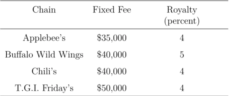
As of 2014, there are over 750,000 franchised establishments in the U.S., earning over $800 billion in revenues and employing over 8 million people (IHS Global Insight, 2015). Franchising is used in a variety of industries including restaurants, fitness centers, convenience stores, and hotels. While contract forms vary across companies, the most common fee structure is one in which the franchisee pays the franchisor a fixed fee for the right to open a store and then a royalty that is a fixed percentage of sales. For a given franchisor, the fixed fee and royalty rate are usually the same for all franchisees and all stores. Furthermore, for a given franchisor, franchise fees are generally persistent over time.
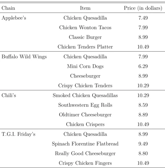
Association, 2016). In a 2010 USDA survey, over 80% of individuals reported eating a meal prepared away from home in the last week, and over 20% reported eating six or more meals prepared away from home. After fast food restaurants, casual dining restaurants make up the largest segment of the restaurant industry. Casual dining restaurants are characterized by moderate prices, full table service, and the availability of a variety of alcoholic beverages. With over 1,800 restaurants and $4.7 billion in annual revenue, Applebee’s is the largest casual dining chain in the United States. Because I intend to measure the effect of franchising on Applebee’s, I focus on Applebee’s and its closest competitors. Specifically, I look at casual dining restaurants that, like Applebee’s, are affiliated with a national chain and have a wide variety of menu items. In addition to traditional American fare like hamburgers and steak, their menus include items inspired by Italian, Asian, and Mexican cuisine. I include the following stores in this grouping: Buffalo Wild Wings, Chili’s, and T.G.I. Friday’s. Together with Applebee’s, these are four of the top seven casual dining chains in the United States. Table 1.2 shows a selection of menu items and prices for each of these four chains; the table shows that the chains have similar menu items and similar prices. As of 2015, the average check size at Applebee’s was $12.42 and the average check size at Chili’s was $13.99.10 While
franchising is very common among fast food chains, it is used less frequently by casual dining chains. For example, all T.G.I. Friday’s, Olive Garden, Outback Steakhouse, and Red Lobster restaurants in Texas are company-owned. About half of the Buffalo Wild Wings restaurants and all of the Applebee’s and Chili’s restaurants in Texas are franchised. One final piece of relevant information is that the casual dining industry is known to be highly competitive and characterized by low profit margins; in 2010, full-service restaurants with average check sizes of less than $15 had a median pretax profit margin of 3% (National Restaurant Association, 2010).
10While average check sizes for Buffalo Wild Wings and T.G.I. Friday are unavailable, given the
For the casual dining chains that use franchising, fees follow the standard format discussed above and are identical for all stores affiliated with a given franchisor. As shown in Table 1.1, fees are similar across many large chains. Franchise contracts typically have a long term, around 20 years, so the fixed fee represents a small share of the total fees paid. Because franchisors typically aim to maintain a consistent brand identity, franchise contracts often contain specific rules about conforming to franchisor policies. As a result, restaurants affiliated with the same chain tend to have similar menu offerings and prices.11
1.2.1 Sale to IHOP
In 2007, there were 59 company-owned Applebee’s stores and 33 franchised Applebee’s stores in Texas. In February of that year, Applebee’s, a publicly traded company, put itself up for sale. Five months later, IHOP Corporation agreed to purchase the chain for $1.9 billion. IHOP Corporation is the parent company of IHOP, the largest chain restaurant in the family dining category.12 IHOP Corporation has a strong preference
toward franchising its stores; at the time of the sale, nearly 100% of IHOP restaurants were owned by franchisees. Shortly after the sale, IHOP Corporation began selling its company-owned Applebee’s stores to franchises. By the end of 2008, all Applebee’s stores in Texas were franchised.13 Annual store counts by ownership type are presented
in Figure 1.1.
One relevant question is why IHOP chose a different ownership strategy than Apple-bee’s had chosen. A possible indication of IHOP’s reasoning is found in a presentation
11An example of Applebee’s attempt to balance this preference for uniformity with a desire to cater to
local markets can be found in its 2013 franchise disclosure document. Applebee’s creates a uniform menu for all of its stores and requires all franchisees to use it. However, the chain also allows for franchisees to “propose additional items that appeal to local trends and traditions.”
12The main difference between the family dining category and the casual dining category is that
family dining restaurants typically do not sell alcohol. Following the sale, IHOP Corporation changed its name to DineEquity. Throughout the paper, I use “IHOP” to refer to the parent company that owns Applebee’s.
13This is not a single-state phenomenon; Applebee’s 2014 10-K states that 99 percent of IHOP and
to investors given by IHOP in 2012 regarding the decision to sell company-owned Apple-bee’s stores to franchisees. In the presentation, IHOP states “[t]he Company believes a more heavily franchised business model requires less capital investment and reduces the volatility of its cash flow performance.” Thus, IHOP may have given greater weight to those concerns than it did to a simple comparison of whether, for a given store, its profits would be greater as a store owner or as a franchisor. Also in the presentation, IHOP predicted that each restaurant sale would result in an annual cost savings of $90,000 due to reduced administrative costs and reduced capital expenditures.
1.3 Motivational Model of Ownership Selection
In this section I construct an model of a profit-maximizing franchisor who decides whether a given store should be company-owned or franchised. While I do not attempt to estimate this model, it provides intuition that is used in my empirical models. The model gives two significant results. First, it predicts that the franchisor will choose to own stores at the best locations and franchise stores at the other locations. Second, it highlights the sort of exogenous variation needed to give an unbiased estimate of the franchise effect.
A franchisor plans to open a store at location j and must decide whether the store
should be company-owned or franchised. If storej is company-owned, the present value
of all future revenues for store j at the time of store j’s opening is
rjC =σaj +ξj, (1.1)
where aj contains location-level attributes that are observed by the econometrician and
ξj represents location-level determinants of revenue that are not observed by the
econo-metrician. Components of aj may include demographics such as the population and
average income of the local market;σ is a vector of parameters. Theξj term is included
restaurants).
As discussed earlier, there are reasons to believe that a franchised store will outper-form a company-owned store. I define β as the present discounted value of all additional
revenues earned by a store if it is franchised. So, revenue for a franchised store is
rFj =rjC +β.
Costs are normalized to zero, so maximizing revenue is equivalent to maximizing profit. For a company-owned store, the franchisor keeps all revenue as profit:
ΠC j =r
C
j . (1.2)
For a franchised store, the franchisor earns a share, v, of all revenue collected as well as
a fixed fee, K. Franchisor profit from a franchisee-owned store is
ΠF j =v
rjC +β+K.
The franchisor will choose to franchise store j if ΠFj >ΠCj. This occurs when
rCj < K +βv
1−v . (1.3)
Thus, stores with low values of rC
j will be franchised. The intuition for this prediction is
that the franchisor receives all of the profits of a company-owned store and only a fraction of the revenue of a franchised store. For the best locations (those with the highest values of rC
order to keep all of the location’s profits.14
To illustrate the impact that this selection has on attempts to measure β, consider
two stores, k and l, that have identical observables, ak =al. Store k is company-owned
and storel is franchised. I definerj as the revenue of storej and fj as a dummy variable
equal to 1 if store j is franchised:
rj =fjrjF + (1−fj)rjC.
The difference in store revenues is
rl−rk=ξl−ξk+β.
If the two stores have identical unobservables, or if ownership is randomly determined such that
E[fj|ξj] =E[fj], (1.4)
then rl−rk is an unbiased estimate of β. However, it is likely thatξj will be correlated
with the ownership decision. There is a direct relationship between ξj and rjC shown in
(1.1). As shown in (1.3), stores with high values of rCj will be company-owned, so it is
likely that ξk > ξl. This means that an estimation of ˆβ =rl−rk is likely to be biased
downward. Observing both rC
j and rjF for some store j would overcome this obstacle.
Because this will involve observing the same store at different times, I define fjt as a
dummy variable equal to 1 if store j is franchised at time t. The condition for a valid
instrument can now be shown as
14The model makes two significant assumptions. The first is that there are no costs. The second
is that β is an additive increase to profits instead a multiplicative increase. (A multiplicative increase would be shown as rF
j =βrjC.) However, either of these two assumptions can be loosened. While the condition for franchising shown in (1.3) will change, the conclusion that stores lower values of rC
jare
E[fjt|ξj] =E[fjt] (1.5)
for some store j that changes ownership. The best way to achieve this would be for an
exogenous event uncorrelated with store-level unobservables to cause the ownership of a store to change. The sale of Applebee’s to IHOP satisfies these requirements; after 2008,
E[fjt|ξj] =E[fjt] for all stores because fjt = 1 for all stores.
The sale of Applebee’s to IHOP and the subsequent franchising of all company-owned stores allows me to identify the effect of franchising. This event has two qualities that make it a valid instrument. First, it results in some stores being observed both as company-owned and franchised. Second, all stores are franchised by the end of 2008, so the post-2008 ownership of a store is uncorrelated with its unobservables.
1.4 Data
I next describe the three data sets used in my analysis. The first is store-level alcohol revenues for all bars and restaurants in the state of Texas. The second is zip code level population and income data available from government sources. The third consists of disclosure documents required by law to be published by franchisors and furnished to potential franchisees. Summary statistics for store revenues and zip code level populations during the first quarter of 2013 are shown in Table 1.3. More detailed information regarding sample selection and geocoding of locations can be found in Appendix B.
Texas mixed beverage sales tax
My research covers restaurant franchising in the state of Texas, specifically those stores that sell liquor. As of 2015, there are over 43,000 restaurants in Texas with 2016 projected sales of $52.4 billion.15 In 2013, there were over 15,000 restaurants in Texas
that sold liquor, generating more than $5.5 billion in alcohol sales.
Texas imposes a mixed beverage sales tax on all establishments selling liquor to be
consumed on premises, primarily bars and restaurants. While the tax is only imposed on establishments that sell liquor, those establishments must pay the tax on all alcoholic beverages sold, including beer and wine. This tax is equal to a fixed share of revenue (14 percent during my sample period) from the sales of alcoholic beverages. The amount collected is publicly available on a per-store, per-month basis. I use data covering 2004 through the third quarter of 2013.
The data have several features. They cover all restaurants with a liquor license, rather than only a single firm. By dividing the tax revenue by the appropriate tax rate, I obtain store-level alcohol revenues. By observing when firms appear and disappear in the data, I can infer when firms enter and exit. Finally, the data include locations for all firms in the form of street addresses; I use ArcGIS software to identify latitude and longitude coordinates for each store. The data set also has some limitations. The most significant is that it only includes alcohol sales, rather than all revenues received by the restaurant. Thus, I assume that alcohol sales are a proxy for total sales. It is worth noting that alcohol sales typically have a large impact on store success, because alcohol sales generate substantially higher profit margins than food sales.16 A second limitation
is that the data include only revenues, rather than prices and quantities. This means that I cannot differentiate between a store that sells a small quantity of high-priced drinks and a store that sells a large quantity of low-priced drinks.
For Applebee’s, Buffalo Wild Wings, Chili’s, and T.G.I. Friday’s, I used franchise disclosure documents, company websites, and online mapping tools to ensure that all restaurants were properly identified and geocoded. I confirmed that these chains sell liquor and therefore are included in the tax data. (Furthermore, franchise disclosure documents indicate that these chains will not allow a store to open without a liquor license.) The number of stores affiliated with each chain at the beginning of each year
16In 2010, a Nation’s Restaurant News study calculated that median alcohol sales were 350% of costs,
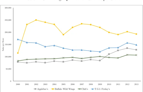
is shown in Figure 1.2. The chains each have similar average per-store revenues, with Buffalo Wild Wings having the highest per-store revenues and Chili’s the lowest. Chili’s, which originated in Texas, has more outlets in Texas than the other chains. Yearly average first quarter per-store alcohol revenues for each chain over time are shown in Figure 1.3.
Stores other than the four chains mentioned above are grouped together at the zip code level, with each group representing an outside option. The average outside option contains 14 stores, with the largest outside option containing 236 stores.
Population data
I use federal income tax return data to estimate annual zip code level populations from 2003 to 2013. The Internal Revenue Service (IRS) releases information on the number of tax returns filed in each zip code. Also included in this data is the number of claimed exemptions filed in each zip code, which the IRS states serves an estimate for population.17 Because this estimate is not exact, I multiply each zip code’s estimated
population by a constant to ensure that total estimated state population matches the actual population each year. During my sample period, this constant ranged from 1.04 to 1.09. Thus, the allocation of population among zip codes may be incorrect, but total statewide population will be correct.18 I next find the latitude and longitude of the
centroid of each zip code using MABLE, an online database maintained by the Missouri State Library. In 2013, there were 1,623 zip codes in Texas with an average population of 16,176 and a median population of 8,672. More densely populated areas contain zip
17The number of claimed exemptions in a region has frequently been used in population estimates. The
U.S. Census Bureau uses this information when calculating annual county-level population estimates and when estimating various statistics, such as poverty rates and health insurance coverage as part of SAIPE (Small Area Income and Poverty Estimates). See Sailer and Weber (1998) for additional discussion.
18While a more accurate population count would be preferred, the finest level where population is
codes that are geographically smaller, while in less populated regions, a single zip code can span a very large area.
Texas experienced significant population growth during my sample period, with statewide population increasing from approximately 22,300,000 to approximately 26,450,000. This growth varied significantly among zip codes, with a quarter of zip codes experiencing no population growth and a quarter of zip codes experiencing a population increase of 20 percent or more. This illustrates the importance of using a model that separates revenue changes due to franchising from revenue changes due to population growth.
I use annual per-capita income data from the U.S. Census Bureau. These data are not available at the zip code level. So, when zip code level per-capita income data is required by the model, I assume each zip code has a per-capita income equal to the per-capita income of the county where the zip code is located. Income quartiles are determined by assuming that each individual has an income equal to the per-capita income of their county and then finding cutoff values such that 25%, 50%, or 75% of individuals have incomes below that value. Income quartiles over time are graphed in Figure 1.4; numbers indicate the lowest income for an individual in each income quartile.
Franchise disclosure documents
Federal law requires franchisors to create a franchise disclosure document (FDD) and distribute the FDD to all potential franchisees. FDDs contain information about the franchisor and the business relationship between the franchisor and its franchisees. Several states require all franchisors operating in that state to submit an FDD to the state, in which case the FDD often becomes a public record. Each FDD includes a list of all franchisee-owned stores.19 I use Applebee’s FDDs from 2006 and 2010-2011 to
determine which stores were company-owned and which were franchised prior to 2008.
1.5 Additional Data Discussion
Table 1.4 gives statistics on populations and alcohol sales for 2013. The ten largest counties are described individually; all other counties are aggregated together. Overall, in 2013 there were 14,816 establishments in the state that sold liquor for on-premises consumption, with total alcohol sales of $5.57 billion, which is an average of $306 per adult of legal drinking age.20 The sale of Applebee’s to IHOP occurred in 2007, which was
shortly before the financial crisis of 2008 and subsequent recession. Thus, it is important to understand how the recession affected alcohol consumption and, more generally, how individuals’ incomes and alcohol choices changed over time. Figure 1.5 shows statewide total sales and per capita sales from 2004 to 2013. Both figures tend to increase through-out my sample period, but these increases stall in 2008 and 2009. Figure 1.6 shows how incomes and total sales as a share of income change over time.21 The share of income
spent on alcohol stays roughly constant throughout most of my sample period; the one notable aberration is a sharp decrease in 2009.
There is substantial variance in alcohol sales among establishments. In the first quarter of 2013, the five largest sellers had average revenues of $3.57 million, while there were 197 establishments with sales of less than $1,000. It is also worth noting that none of the top ten sellers of alcohol are traditional bars or restaurants; all of them are hotels, convention centers, airports, or sports arenas. I choose not to remove any of these large sellers from my analysis for two reasons. First, it is not clear what a reasonable removal strategy would be, and second, these large sellers are not actually outliers in my estimation. This is because I estimate both the linear model and the structural model using logged sales, rather than actual sales. As shown in Figure 1.7 and Figure 1.8, while
20Establishment counts are taken in the first quarter of the year; because firms enter and exit
through-out the year, the total number of establishments will change during each year. Similarly, whenever yearly population is used in graphs or tables, population as of the first quarter of the year is used.
21Because in my structural model individuals set their alcohol budget as a share of their incomes, per
a histogram of sales shows significant outliers on the right side of the distribution, no such outliers exist on a histogram of logged sales.
Finally, Figure 1.9 is a map of all chain stores in Texas in 2006. Additionally, coun-ties in the map are shaded based on their per-capita alcohol sales. Three patterns are noticeable. First, chain stores tend to be located in areas that have high per-capita al-cohol sales. The cause of this relationship is not clear; it could be that individuals who live in counties with high per-capita sales have strong tastes for alcohol, and the chain restaurants respond to those tastes by opening restaurants there. Alternatively, it could be that the existence of so many chain restaurants encourages individuals to consume more alcohol at restaurants than they otherwise would have. Second, while most stores are located in populous areas such as Dallas and Houston, there are also several stores (mostly Chili’s and Applebee’s) in less populous areas. These areas tend to have only one store. This may be evidence that these smaller markets can only support one chain restaurant. Third, company-owned Applebee’s tend to be near other company-owned Applebee’s, and franchised Applebee’s tend to be near other franchised Applebee’s.
1.6 Franchisor’s Ownership Selection Process
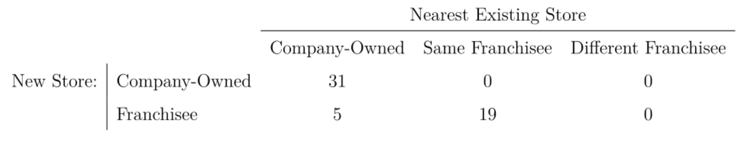
As discussed earlier, past research has found evidence that, when franchisors open new stores, the franchise status of the new store tends to be identical to that of nearby stores.22 Figures 1.10 and 1.11 show the locations of company-owned and franchised
stores in Texas. The company-owned stores are mostly clustered in the Dallas and Houston areas, while franchisees own stores in large cities such as El Paso and Austin as well as in more isolated markets throughout the state.
Using Texas mixed beverage alcohol sales data from 2000 to 2014, I identify 65 new
Applebee’s being opened.23 For each store, I identify, at the time of opening, the existing
store that is closest to the opening store. I then compare the ownership of the two stores. I exclude from my analysis any opening store that is not within 50 miles of an existing store and any opening store in which the ownership of either the opening store or the nearest existing store is unknown. This leaves 55 opening stores. Of those 55 stores, 50 have the same owner as the nearest existing store. Thus, there is significant evidence supporting the hypothesis that the franchisor prefers nearby stores to share the same owner. Full results are shown in Table 1.5. There are two possible reasons for this. First, the franchisor may wish to capitalize on the local experience of a franchisee, and second, nearby stores will be easier for an existing franchisee to monitor.
It is useful to compare these results to the results of the theoretical model presented in Section 1.3. In that section, the ownership of each store was determined solely by the quality of each location, with quality being independent of the ownership of the store. In order for this theory to be consistent with the observed ownership patterns, it would need to be the case that location quality tends to be very similar at proximate locations. For example, all Applebee’s stores in El Paso County were franchisee-owned prior to 2008. According to the model, this means that all El Paso locations are low-quality. Similarly, all Applebee’s stores in Dallas County were company-owned prior to 2008 and, therefore, are predicted by the model to be high-quality. Given the array of location types within a county,24 it seems unlikely that the worst location in Dallas County is
better than the best location in El Paso County. Instead, it seems probable that the franchisor’s ownership decision depends not just on the quality of the location but on the owner of nearby stores as well. This does not necessarily mean that the franchisor is
23Note that this is a longer period of time than the data I use throughout my other analyses. This
is because some of the demographic data used in those models was only available for a subset of those years. I consider a store’s opening date to be the first quarter that it has alcohol sales recorded in the data set.
24For example, El Paso County contains Applebee’s stores in strip malls, outside of shopping malls,
not pursuing a profit-maximizing ownership strategy. Instead, it may indicate that each store’s potential revenue is highly dependent on the local expertise or monitoring ability of its owner.
Most importantly, these results do not affect the most important prediction of Section 1.3: store ownership is likely correlated with unobservables. The reason that this is likely still true is because, even if unobservables do not directly influence the ownership decision because the impact of unobservables on profit is small relative to the impact of a local owner (which, given that the ownership of a new store is so highly correlated with the ownership of the nearest existing store, appears to be the case), it is likely that nearby stores have similar observables. Continuing the earlier example, it is likely that the unobservable determinant of revenue at a given El Paso Applebee’s is closer to the unobservable component at another El Paso Applebee’s than it is to the unobservable component at a Dallas Applebee’s, because the factors that determine this unobservable (such as, for example, quality of competing restaurants or grocery stores, religious beliefs about alcohol, and socioeconomic factors not included in my population demographics) will be similar for nearby stores.
in absolute terms and on a per-person basis. Because these stores are competitors, it may appear surprising that the franchisor chose to own stores in counties with more competition. However, it is possible that there are counties which have a strong taste for chain restaurant fare; this feature could have both benefited Applebee’s and led to more competitors entering the market. I next compare the 2006 fourth quarter revenues of company-owned and franchised Applebee’s. A histogram of revenues for both ownership types is shown in Figure 1.12. Summary statistics for the two ownership types are shown in Table 1.7. Company-owned stores have an average revenue of $80,987, while franchised stores have a slightly lower average revenue of $78,816. The median revenue of company-owned stores (79,561) is considerably larger than the median revenue of franchised stores (66,847) because the average revenue for franchised stores is skewed by some high-revenue outliers. There is substantial variance in revenues within each ownership type.
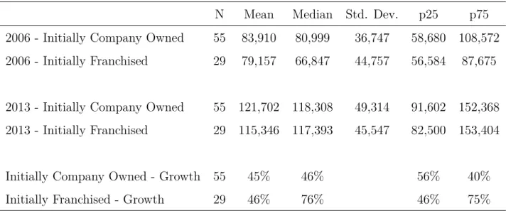
I now look for initial evidence of a benefit from franchising. I do this by comparing the 2006 fourth quarter revenues with the 2013 fourth quarter revenues for the two ownership types.25 In my comparison, I only include stores that were open during that entire time
period. This results in a sample size of 55 company-owned stores and 29 franchised stores. During these seven years, all company-owned Applebee’s were sold to franchisees; thus, all else equal, if there is a positive franchise effect, I would expect the stores that were initially company-owned to have a greater revenue increase than the stores that are franchisee-owned (or, if there is a downward trend in store revenues, a smaller revenue decrease).
Summary statistics for the two time periods are shown in Table 1.8. Stores that were initially company-owned (and, therefore, experienced a change in franchise status) actually had a slightly smaller average revenue increase on a percentage basis (46% for franchised stores and 45% for company-owned stores), and stores that were franchised
25I use these end points because the fourth quarter of 2006 is the last quarter before the year that the
actually had a much bigger increase in median sales (76% for franchised stores and 45% for company-owned stores). Histograms of store revenue for both ownership types and both time periods are shown in Figure 1.13.
Table 1.1: Franchise Fees for Various Casual Dining Chains
Chain Fixed Fee Royalty
(percent)
Applebee’s $35,000 4
Buffalo Wild Wings $40,000 5
Chili’s $40,000 4
T.G.I. Friday’s $50,000 4
Notes: These numbers come from franchise disclosure documents and do not include any additional fees paid to
Table 1.2: Sample of Menu Items and Prices
Chain Item Price (in dollars)
Applebee’s Chicken Quesadilla 7.49
Chicken Wonton Tacos 7.99
Classic Burger 8.99
Chicken Tenders Platter 10.49
Buffalo Wild Wings Chicken Quesadilla 7.99
Mini Corn Dogs 6.29
Cheeseburger 8.99
Crispy Chicken Tenders 10.29
Chili’s Smoked Chicken Quesadillas 10.29
Southwestern Egg Rolls 8.59
Oldtimer Cheeseburger 8.89
Chicken Crispers 10.49
T.G.I. Friday’s Chicken Quesadilla 8.99
Spinach Florentine Flatbread 9.49
Really Good Cheeseburger 8.80
Crispy Chicken Fingers 10.49
Notes: Prices are taken from the following Dallas outlets: Applebee’s on 3565 Frankford Rd; Buffalo Wild Wings on 5000 Belt Line Rd.;
Table 1.3: Summary Statistics for the First Quarter of 2013
N Mean Std. Dev. Min Max p25 p75
Store Revenues
Applebee’s 100 127,908 52,606 33,876 301,348 86,007 164,084
Buffalo Wild Wings 83 192,246 77,876 43,304 631,270 151,312 208,414
Chili’s 208 107,038 31,658 20,791 215,367 86,430 123,094
T.G.I. Friday’s 31 132,098 56,288 56,004 318,888 102,871 143,570
Outside option 973 1,343,398 3,223,087 491 58,994,137 85,178 1,347,029
Stores per
outside option 973 14 19 1 236 3 19
Zip code level
populations 1,623 16,176 18,320 110 115,975 2,240 25,370
Notes: Each outside option includes all non-chain stores in a zip code.
Table 1.4: County Level Statistics for 2013
County Population Number of
Stores (in thousands ofAlcohol Sales dollars)
People per
Store Sales perPerson
Harris 4,325,413 2,552 1,198,724 1,695 277
Dallas 2,459,095 1,882 837,970 1,307 341
Tarrant 1,910,975 1,441 536,603 1,326 281
Bexar 1,813,421 1,032 511,175 1,757 282
Travis 1,108,503 962 591,169 1,152 533
Collin 854,036 609 209,761 1,402 246
El Paso 829,726 400 131,629 2,074 159
Hidalgo 818,553 282 74,362 2,903 91
Denton 721,022 356 107,133 2,025 149
Fort Bend 650,693 222 76,489 2,931 118
All other counties 10,958,769 5,078 1,295,455 2,158 118
Statewide 26,450,206 14,816 5,570,470 1,785 211
Notes: All establishments found in the Texas mixed beverage sales tax data are included in the
count of stores. Store counts and populations reflect data for the first quarter of 2013.
Table 1.5: Ownership of New Stores and Nearest Existing Stores
Nearest Existing Store
Company-Owned Same Franchisee Different Franchisee
New Store: Company-Owned 31 0 0
Franchisee 5 19 0
Notes: Opening stores that are not within 50 miles of an existing store and opening stores in which the ownership of either the opening store or the nearest existing store is unknown are excluded
from this analysis.
Table 1.6: County-Level Averages by Applebee’s Ownership Type, Q4 2006
Counties with Company-Owned
Stores
Counties with Franchised Stores
Number of Applebee’s 2.18 1.74
Number of Other Chain Stores 7.36 3.26
Number of Non-Chain Stores 284.50 136.53
Total Alcohol Sales $24,800,642 $10,767,421
Population 475,502 286,301
Per Capita Alcohol Sales $52.16 $37.61
People per Non-Applebee’s Chain Store 64,631 87,737
People per Non-Chain Store 1,671 2,097
Number of Counties: 28 19
Notes: In the fourth quarter of 2006, no county included both company-owned and franchised stores
Table 1.7: Summary Statistics for Applebee’s Alcohol Revenues by Ownership Type, Q4 2006
N Mean Median Std. Dev. p25 p75
Company-Owned 59 53,591 79,561 104,858 80,987 37,392
Franchised 33 54,473 66,847 88,166 78,816 43,973
Table 1.8: Summary Statistics for Applebee’s Alcohol Revenue by Ownership Type, Q4 2006 and Q4 2013
N Mean Median Std. Dev. p25 p75
2006 - Initially Company Owned 55 83,910 80,999 36,747 58,680 108,572
2006 - Initially Franchised 29 79,157 66,847 44,757 56,584 87,675
2013 - Initially Company Owned 55 121,702 118,308 49,314 91,602 152,368
2013 - Initially Franchised 29 115,346 117,393 45,547 82,500 153,404
Initially Company Owned - Growth 55 45% 46% 56% 40%
Initially Franchised - Growth 29 46% 76% 46% 75%
Notes: Only stores which exist in both Q4 2006 and Q4 2013 are included.
Table 1.9: Average Revenue by Quarter
Quarter Revenue
Q1: January - March $101,247
Q2: April - June $97,709
Q3: July
-September $95,278
Q4: October
-December $99,894
Notes: Only stores which were open in all years
from 2004 through 2011 are included. Only sales
Figure 1.1: Number of Applebee’s Stores by Year
0 20 40 60 80 100 120
2000 2001 2002 2003 2004 2005 2006 2007 2008 2009 2010 2011 2012 2013 2014
Company-Owned Franchised
Figure 1.2: Number of Stores for Each Chain
0 50 100 150 200 250
2000 2001 2002 2003 2004 2005 2006 2007 2008 2009 2010 2011 2012 2013
N
um
be
r o
f S
to
re
s
Applebee's Buffalo Wild Wings Chili's T.G.I. Friday's
Figure 1.3: Average Q1 Alcohol Revenue per Store
0 50,000 100,000 150,000 200,000 250,000 300,000
2000 2001 2002 2003 2004 2005 2006 2007 2008 2009 2010 2011 2012 2013
Sa
le
s
pe
r
St
or
e
Applebee's Buffalo Wild Wings Chili's T.G.I. Friday's
Figure 1.4: Income Quartile Cutoffs for Q1 of Each Year
$0 $10,000 $20,000 $30,000 $40,000 $50,000 $60,000
2004 2005 2006 2007 2008 2009 2010 2011 2012 2013
In
co
m
e
Figure 1.5: Statewide Alcohol Revenues
$0 $50 $100 $150 $200 $250
$0 $1,000 $2,000 $3,000 $4,000 $5,000 $6,000
2004 2005 2006 2007 2008 2009 2010 2011 2012 2013
P
er
c
ap
ita
S
al
es
To
ta
l S
al
es
(
in
m
ill
io
ns
)
Total Sales Per Capita Sales
Figure 1.6: Statewide Income and Alcohol Spending 0.0% 0.1% 0.2% 0.3% 0.4% 0.5% 0.6% 0 5,000 10,000 15,000 20,000 25,000 30,000 35,000 40,000 45,000 50,000
2003 2004 2005 2006 2007 2008 2009 2010 2011 2012 2013 2014
Sh ar e of in co m e sp en t on a lc oh ol P er c ap ita in co m e
Per Capita Income Alcohol spending as a share of income
Figure 1.7: Histogram of Alcohol Sales for Q1 2013 0% 5% 10% 15% 20% 25% 30% 2 0, 00 0 4 0, 00 0 6 0, 00 0 8 0, 00 0 1 00 ,0 00 1 20 ,0 00 1 40 ,0 00 1 60 ,0 00 1 80 ,0 00 2 00 ,0 00 2 20 ,0 00 2 40 ,0 00 2 60 ,0 00 2 80 ,0 00 3 00 ,0 00 3 20 ,0 00 3 40 ,0 00 3 60 ,0 00 3 80 ,0 00 4 00 ,0 00 4 20 ,0 00 4 40 ,0 00 4 60 ,0 00 4 80 ,0 00 5 00 ,0 00 5 20 ,0 00 5 40 ,0 00 5 60 ,0 00 5 80 ,0 00 6 00 ,0 00 6 20 ,0 00 6 40 ,0 00 6 60 ,0 00 6 80 ,0 00 7 00 ,0 00 M or e
Figure 1.8: Histogram of Logged Alcohol Sales for Q1 2013
0% 2% 4% 6% 8% 10% 12% 14% 16% 18%