arXiv:1608.03283v1 [astro-ph.SR] 10 Aug 2016
Mon. Not. R. Astron. Soc.000, 000–000 (0000) Printed 12 August 2016 (MN LATEX style file v2.2)
The Magnetic Cataclysmic Variable LSQ1725-64∗
J.T. Fuchs,
1†
Bart H. Dunlap,
1E. Dennihy,
1D. O’Donoghue,
2,3J.C. Clemens,
1D.E. Reichart,
1J.P. Moore,
1A.P. LaCluyze,
1J.B. Haislip,
1and K.V. Ivarsen,
11 Department of Physics and Astronomy, University of North Carolina at Chapel Hill, Chapel Hill, NC 27599, USA 2
South African Astronomical Observatory, PO Box 9, Observatory 7935, South Africa
3
Southern African Large Telescope, PO Box 9, Observatory 7935, South Africa
Accepted 2016 July 18. Received 2016 July 18; in original form 2016 March 22
ABSTRACT
We present new photometry and spectroscopy of the 94m eclipsing binary LSQ1725-64 that provide insight into the fundamental parameters and evolutionary state of this system. We confirm that LSQ1725-64 is a magnetic cataclysmic variable whose white dwarf has a surface-averaged magnetic field strength of 12.5±0.5 MG measured from Zeeman splitting. The spectral type and colour of the secondary, as well as the eclipse length, are consistent with other secondaries that have not yet evolved through the period minimum expected for cataclysmic variables. We observe two different states of mass transfer and measure the transition between the two to occur over about 45 orbital cycles. In the low state, we observe photometric variations that we hypothe-size to arise predominantly from two previously heated magnetic poles of the white dwarf. Our precise eclipse measurements allow us to determine binary parameters of LSQ1725-64 and we find it contains a high mass (0.97±0.03M⊙) white dwarf if we
assume a typical mass-radius relationship for a CO core white dwarf. We also measure an eclipse of the accretion stream after the white dwarf eclipse, and use it to estimate an upper limit of the mass transfer rate. This derived limit is consistent with that expected from angular momentum loss via gravitational radiation alone.
Key words: stars: cataclysmic variables, binaries: eclipsing, stars: individual: LSQ172554.8-643839, magnetic fields, accretion
1 INTRODUCTION
Most cataclysmic variables are white dwarf - main sequence binaries in orbits so close that the main sequence companion sporadically or continuously transfers matter to the white dwarf. Warner(1995) provides a thorough summary of the field. Around 25 per cent of the white dwarfs in cataclysmic variables have magnetic field strengths of at least a few MG (Wickramasinghe & Ferrario 2000).
Polars, or AM Her stars, are an observationally dis-tinguished subclass that contain white dwarfs with mag-netic fields greater than about 10 MG. They exhibit strong (greater than ten per cent) linear and circular polarization
∗ Based on observations obtained at the Southern Astrophysical Research (SOAR) telescope, which is a joint project of the Min-ist´erio da Ciˆencia, Tecnologia, e Inova¸c˜ao (MCTI) da Rep´ublica Federativa do Brasil, the U.S. National Optical Astronomy Ob-servatory (NOAO), the University of North Carolina at Chapel Hill (UNC), and Michigan State University (MSU). Also based on observations made with the Southern African Large Telescope (SALT).
(Cropper 1990). Their spectra show strong Balmer emis-sion lines along with He I and He II. He II is typically stronger in polars compared to non-magnetic cataclysmic variables (Szkody 1998). Cyclotron radiation from spiraling matter in the accretion stream can be seen in time-resolved spectroscopy. The wavelength of the cyclotron harmonics de-pends on the magnetic field strength of the white dwarf and is commonly in the infra-red or optical (Cropper et al. 1989). Measuring the Zeeman splitting of the Balmer lines can give an estimate of the white dwarf magnetic field strength and geometry (Beuermann et al. 2007).
Polars tend to have lower rates of mass transfer, around 10−11
M⊙yr−1, compared to non-magnetic cataclysmic
mostly been in a low state since 1997 (Wheatley & Ramsay 1998) with only brief returns to the high state since 2006.
LSQ172554.8-643839 (hereafter LSQ1725-64) is an eclipsing binary with a period of ∼94 minutes. Its V-band
magnitude varies between 18 and >24 throughout the or-bital cycle. It was first discovered as a variable star by Ra-binowitz et al.(2011). Follow-up optical photometry showed an eclipse that lasted for∼5 minutes with an ingress depth
of more than 5.7 mag; amongst the deepest eclipses known for all cataclysmic variables.Rabinowitz et al.(2011) mea-sured a magnitude for the secondary star during eclipse in the J band only; without a colour measurement they were only able to place a limit on the spectral class. They did not measure any evidence for a magnetic field, so could not def-initely conclude that LSQ1725-64 is a magnetic cataclysmic variable.
The properties of LSQ1725-64 as described by Rabi-nowitz et al. (2011) make it an intriguing and appealing object for follow-up study. It could offer insight into mag-netic accretion physics, the role of magmag-netic fields in bi-nary star evolution, and the period evolution of cataclysmic variables. This last item is intimately related to the mass-radius relation of the secondary star and the mechanisms that might drain angular momentum from binaries: mag-netic braking and gravitational radiation. Short period sys-tems like LSQ1725-64 are particularly interesting to study, as there should be some period at which continued mass transfer causes the secondary to expand above its equilib-rium radius, resulting in evolution to longer rather than shorter periods. The location of this period bounce and the evolution of systems that have passed through it are critical to our understanding of angular momentum loss and period evolution in cataclysmic variables.
Based on derived binary parameters and a V-J limit during eclipse,Rabinowitz et al.(2011) suggested LSQ1725-64 might be a post-bounce system, i.e. one that is already evolving to longer orbital periods as the now degenerate sec-ondary expands in response to mass loss. This would make it a rare and valuable object of study as there are very few known (see e.g. Littlefair et al. (2006) and G¨ansicke et al. (2009)). On the basis of these interesting possibili-ties, we conducted a campaign of time-resolved spectroscopy, short cadence photometry, and photometric monitoring of LSQ1725-64.
Insection 2, we describe our observations and reduction process. Insection 3, we show spectroscopic measurements of the Hβabsorption line of the white dwarf that permit us to conclude with certainty that the system contains a magnetic white dwarf. Insection 4, we summarize the photometric be-haviour of LSQ1725-64 on time-scales ranging from seconds to years. We present results from time-resolved optical spec-troscopy in section 5. Section 6 discusses the evolutionary status and presents updated binary parameters of LSQ1725-64. Finally, we conclude in section 7by fitting LSQ1725-64 into context as a polar and adding our measurements to what is already known.
2 OBSERVATIONS
Our new observational data include three kinds of obser-vations of LSQ1725-64: time-series spectroscopy, short
ca-dence photometry, and photometric monitoring of accre-tion state. As summarized in Table 1and Table 2, we ob-served LSQ1725-64 on 14 separate nights with an imag-ing spectrograph—the Goodman Spectrograph on the 4.1-m SOAR Telescope (Clemens et al. 2004).
For the SOAR Goodman photometry, we binned the CCD at 2×2 with the exception of 2012-08-12, when we
binned at 1 × 1. We did not use a filter for most of the
photometry, allowing us to decrease the exposure times and increase the amount of time-dependent geometrical informa-tion in the data. For select eclipse measurements we obtained photometry in SDSSu′,g′,r′, andi′ bands. To reduce the readout time, the typical region of interest used was 90 ×
90 arcsec, resulting in a readout time of ∼3 s and a duty
cycle greater than 80 per cent. All observations beginning in 2013 have GPS derived shutter open times recorded in the image header.Table 1gives details of all our photometry.
For our spectroscopic observations, we used a 1.68′′slit,
but did not stay aligned to the parallactic angle. There was no atmospheric dispersion corrector installed on the Good-man Spectrograph at the time of these observations. We took continuous sequences of spectra with no gaps, which limited the measurement of standards to only one a night. As a result of this observing strategy, our flux calibrations are less than ideal, but our velocity measurements, with er-rors ∼ 40 km s−1, are as good as the instrument can do
given our resolution.
Nearly all spectroscopic observations had exposure times of 300 s, equalling a phase width of 5.2 per cent. Dur-ing eclipse, or the low state, the typical signal-to-noise of the continuum from an individual spectrum was around 6 per binned pixel. In the high state, the typical signal-to-noise of the continuum from an individual spectrum of the accreting hemisphere was between 8 and 13 per binned pixel.Table 2 gives details of all our spectroscopy.
We also observed LSQ1725-64 three times with the SALTICAM Imager on the Southern African Large Tele-scope (SALT; O’Donoghue et al. (2006)). We used frame transfer mode on SALTICAM, which allows half the chip to be shifted on to the unexposed half of the chip nearly instantaneously, limiting dead time between exposures. As with the Goodman photometry, we did not use a filter. The observations with SALT did not cover a full orbit, but in-stead were centred on the eclipse to resolve the ingress and egress structure.
We used the PROMPT network of robotic telescopes to monitor the accretion state of LSQ1725-64. As with the other photometry, we did not use a filter. Exposure times were 180 s, with a readout time of∼6 s, providing a duty
cycle of 96.7 per cent. PROMPT monitored LSQ1725-64 on 70 separate nights during low, high, and intermediate states. We typically obtained one orbit per night.
The Polar LSQ1725-64
3
Table 1.Photometric Observations with the Goodman Spectrograph on the SOAR Telescope and SALTICAM on SALT.
Observation Start Instrument Exposure Length of Eclipses Accretion
Date (UT) Time (s) Observation (hours) Observed State
2011-09-07 SALTICAM 15.7 1.8 1 High
2012-08-12 Goodman 20 4.5 3 High
2013-06-08 Goodman 20 1.7 1.5 Low
2013-07-03 Goodman 20 2.3 2 High
2013-07-06 SALTICAM 1.7 0.8 1 High
2013-07-12 Goodman 12 2.9 2 High
2013-07-27 Goodman 12 1.6 1 High
2013-08-05 Goodman 12 3.6 2 High
2013-08-14 Goodman 11 2.0 2 High
2013-08-15 Goodman 12 1.2 1 High
2013-09-02 SALTICAM 1.7 0.8 1 High
2013-11-14 Goodman 12 1.8 1 High
2014-06-30 Goodman 12 2.5 2 High
Table 2.SOAR Goodman Spectroscopic Observations
Observation Start Grating Exposure Resolution Length of Accretion Date (UT) (l mm−1) Time (s) (˚A) Observation (hours) State
2012-09-26 400 300 12.7 1.43 High
2013-06-07 400 300 12.8 1.16 Low
2013-06-08 400 300 15.3 1.68 Low
2013-06-16 400 300 10.2 3.20 High
2013-07-02 400 300 12.0 1.60 High
2013-07-03 930 300, 600, 60 4.9 2.00 High
2013-07-12 400 300 12.6 2.26 High
2013-07-27 400 300 10.2 2.52 High
night of 2013-07-02. All photometry is presented relative to this average.
Spectroscopic observations were bias subtracted but were also not flat-fielded. The spectra were extracted and wavelength calibrated using the standardIRAF tasks and a HgAr lamp. We produced rough flux calibrations by mea-suring the instrument response with a standard star. We did not sample the same range of airmasses in these standards as in the data, so the main sources of error in the flux cali-bration are changes in extinction and differential slit losses.
3 THE MAGNETIC FIELD OF THE WHITE
DWARF
The observed low state in LSQ1725-64 allowed us to mea-sure the Zeeman splitting of H β in our spectroscopic ob-servations. For magnetic fields less than∼20 MG, the linear
Zeeman effect produces a triplet pattern around the central absorption feature, calculable by
∆λL≃4.7×10⁻⁷ λ2 Bs , (1) where λ is in ˚A, Bs is the surface magnetic field in MG, and ∆λLis the separation of the split components from the central component (Landstreet 1980).
The Hβline has a high signal-to-noise and is relatively free from emission.Figure 1shows an orbital-averaged spec-trum of LSQ1725-64 in the low state. We fitted the H β
line with three equally spaced gaussians to model the Zee-man absorption and used a second-order polynomial for the continuum. The result is shown in red. From Equation 1 we determine a surface-averaged magnetic field of 12.5±0.5
MG.
This magnetic field strength of the white dwarf falls within what is expected for polars. Our measurement of Zeeman splitting offers the best confirmation that the white dwarf in LSQ1725-64 has a strong magnetic field, and al-lows definitive classification of the binary as a cataclysmic variable of the AM Her type.
4 PHOTOMETRIC PROPERTIES OF
LSQ1725-64
In this section, we will present and discuss photometric data gathered on time-scales ranging from seconds to months, but first we update the orbital ephemeris of the binary.
4.1 Orbital Ephemeris
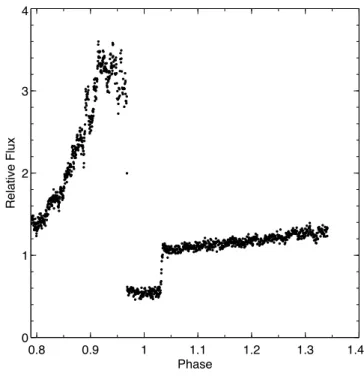
The eclipses in this system yield a very precise measurement of the orbital period. The SALT lightcurve shown inFigure 2 displays a single eclipse at 1.7 s time resolution, taken when the polar was in a high state. In this state, the eclipse ingress is preceded by flickering and includes both the eclipse of the white dwarf and of the accreting pole, which is very near to the limb. This makes it difficult to measure the time of mid-ingress. The eclipse egress does not show this behaviour and lasts 23.4±0.3 s. Thus, we measured eclipse times for
all of our photometric data using times of mid-egress. The measured mid-egress times were all adjusted to Barycentric Julian Date in the Barycentric Dynamical Time standard (BJDT DB) using the code of Eastman et al. (2010). Only SOAR and SALT eclipse data were used to calculate the ephemeris.
To estimate mid-egress times from our data, we fitted a piece-wise function to the egress of the white dwarf. We modeled the eclipse as a linear change between constant flux levels before and after egress. The fit was done with MPFIT, which uses a Levenberg-Marquardt technique to solve the least-squares problem (Markwardt 2009). The linear model was integrated over the same exposure times as the data during the fitting process. All fitted mid-egress times and their associated errors are shown in AppendixA1.
We constructed an O-C diagram using the mid-egress times of the white dwarf.T0was chosen to be the SALT data point taken on 2013-07-06 as it had small error bars and was near the midpoint of all data presented here. We show the O-C diagram in Online Figure 1. Within the precision of these data, we are not able to detect any changes in the orbital period, as might occur either from angular momentum losses or from reflex motion generated by a third body. Therefore, we iteratively fitted a linear ephemeris to get the following result:
T0= 2456480.4422112(55) +
E × 0.065741721(2) days(BJDT DB) (2)
where the numbers in parentheses are the error on the last digits. This period corresponds to 5680.0847(1) s. Note that
Figure 2.A SALT lightcurve from 2013-07-06 with an exposure time of 1.7 s. The structure of the eclipse ingress of the white dwarf and hotspot is not resolved with this time sampling. The egress of the white dwarf lasts 23.4±0.3 s and appears unaffected by any hotspot.
theT0 is a time of mid-egress and throughout this paper we define orbital phase 0 as the mid-eclipse time. Thus,T0, the time of mid-egress, occurs at orbital phase 0.033. This phase difference was established by measuring the time from end of ingress to beginning of egress, and combining half of that value with half of the egress time. With this ephemeris in hand, we can proceed to look at data over a single orbit or folded over several cycles.
4.2 Photometric Variations at the Orbital Period
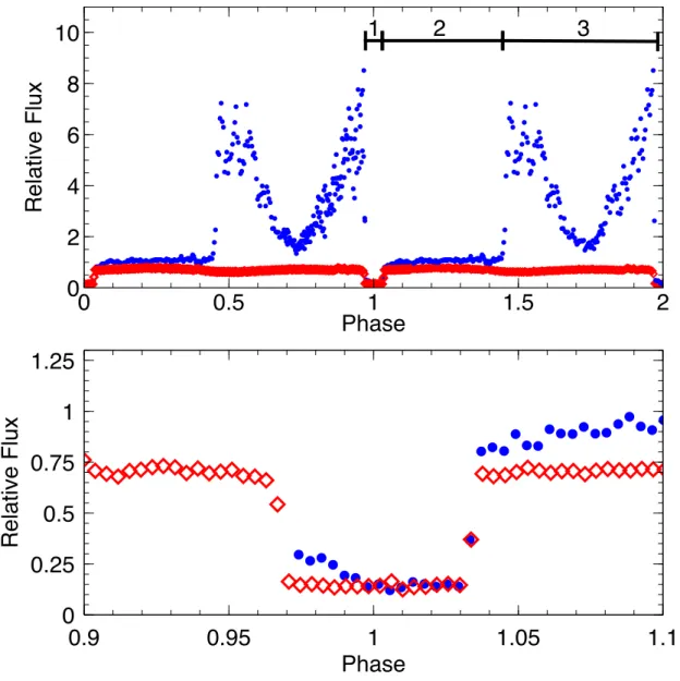
The two lightcurves shown inFigure 3exemplify the white light photometric behaviour of LSQ1725-64 over its orbital cycle. In this section we will describe how the variations in both the high and low state translate into geometrical information about LSQ1725-64.
4.2.1 Photometric Variations During the High State
AsFigure 3shows, our photometry of LSQ1725-64 exhibits the same behaviour as Rabinowitz et al. (2011) found in the high state. In describing the lightcurves of LSQ1725-64, Rabinowitz et al.(2011) divided its orbit into three regions. Following and refining this designation we refer to orbital phases between 0.97 and 1.03 as region one, between 0.03 and 0.45 as region two, and between 0.45 and 0.97 as region three. We have marked these regions inFigure 3. Note that these numbers are adjusted fromRabinowitz et al. (2011) to incorporate the better time resolution of our data.
The Polar LSQ1725-64
5
Figure 3.A comparison of the two states of mass transfer in LSQ1725-64. Blue circles show the high state from 2013-07-02. Red diamonds show the low state from 2013-06-08. The bottom plot shows the same data, but enlarged to show the slow eclipse of the accretion stream above the limb of the white dwarf after the eclipse of the white dwarf and hotspot. The high state data are above the scale shown. We mark regions 1, 2, and 3 as defined byRabinowitz et al.(2011) at the top of the upper panel. We present the photometry as a flux relative to the average of region 2.
owing to the faintness of the secondary, and to the orien-tation of the accreting pole which makes it brightest just before eclipse ingress. A close-up of the eclipse is shown in the bottom panel ofFigure 3. In the high state, the ingress is dominated by the very rapid eclipse of the accretion spot on the white dwarf photosphere (e.g.O’Donoghue et al.(2006)). The relatively slow decline after ingress, which lasts close to two minutes, or about half of the total eclipse time, we at-tribute to the secondary star slowly eclipsing an optically thick accretion stream that funnels material along the mag-netic field and on to the accretion pole which is nearly per-pendicular to the line of sight at this orbital phase (see be-low). This has been seen before byBridge et al.(2003) in EP Dra who interpret it as an eclipse of the accretion stream and use it as a proxy for the Alfv´en radius, as we also do later. The eclipse of this stream is not detected in the low
state lightcurve. The white dwarf egress lasts 23.4±0.3 s,
and we will use this value later to measure the white dwarf radius. We do not see the reemergence of the spot at the end of eclipse, indicating it has disappeared around the limb of the white dwarf.
We interpret region two as the half of the orbit in which the accretion heated pole is on the far side of the white dwarf. In this region, just after egress, the high state lightcurve is brighter than the low state lightcurve, presum-ably because the bright accretion stream adds flux in the high state.
around 5500 ˚A. If we attribute this to cyclotron radiation, it should be beamed at 90 degrees to the magnetic field axis, and therefore brightest just after the accretion pole comes into view at the stellar limb, and again just before it disappears half an orbit later. The lightcurve conforms to this expectation.
From the orbital phases of accretion spot appearance and eclipse, we estimate the longitude of the accretion spot to be 99 ±5 degrees. Using the inclination we calculate in
subsection 6.2,i= 85.6◦±1.7◦, and the phase length that
the accretion spot is in view, ∆φ= 0.55 ± 0.03, we can
estimate the co-latitude of the magnetic pole,β,
tan(i)×tan(β) =−sec(π∆φ) (3)
(seeBeuermann et al.(1987)). This result is highly sensitive to the inclination, but yields an estimate of 10◦< β <59◦.
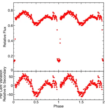
4.2.2 Photometric Variations During the Low State
The SOAR low-state lightcurve in white light, shown in the top panel ofFigure 4, shows a periodic modulation at twice the orbital period, with the maximum occurring near phases 0.25 and 0.75. Upon first glance, this resembles what we ex-pect from ellipsoidal variations of the secondary, but this appearance is deceiving. As the eclipse inFigure 4shows, in the observed band only∼ 1
6 of the light comes from the sec-ondary. After correcting for the dilution by the white dwarf, the variations would be over 50 per cent, as shown in the bottom panel of Figure 4. We show in Appendix B that the largest ellipsoidal variation expected for the mass ratio in LSQ1725-64 is 11.7 per cent. Thus, these modulations cannot be caused solely by ellipsoidal variations of the sec-ondary.
Piro et al.(2005) show that after dwarf novae outbursts, the white dwarf cooling time back to the quiescent tempera-ture can be months to years. Therefore, we expect any mag-netic pole on the white dwarf that has accreted in the past to be hotter than the surrounding white dwarf photosphere. We hypothesize that the low state lightcurve modulation arises from the white dwarf, and is the fluctuation of two previously heated magnetic poles of the white dwarf. Previ-ous observations of polars have detected accretion switching between one and two poles in both QS Tel (Rosen et al. 1996) and MT Dra (Schwarz et al. 2002).
The two maxima in the low state align in phase with our expectation of magnetic pole locations on the white dwarf based on our description in subsection 4.2, and assuming a dipole geometry. If the double-humped variation in the low state arises from the magnetic poles then the tempera-ture of each pole might conceivably be measured, and would constrain the time-averaged accretion rate on to each pole (Townsley & G¨ansicke 2009).
4.3 Long Term Monitoring of Photometric States
Figure 5shows the average region three flux for each night of PROMPT data, where, for consistency, we only include nights when the entirety of region three was sampled at least once. Between 6 June 2013 and 12 November 2013 we de-tected LSQ1725-64 in a high state on 45 out of 70 nights. These nights are when we observed with PROMPT at our
Figure 4.The low state lightcurve of LSQ1725-64 showing the amplitude variations (top). The eclipse shows the brightness of the secondary star and if the variations arise from its elliptical shape they would be at least 50 per cent of the secondary flux. We show this in the bottom panel. We hypothesize that the variations predominantly come from the two previously heated magnetic poles of the white dwarf.
highest cadence, and this number is likely a lower limit on the percentage of time LSQ1725-64 spends in a high state because the near-nightly monitoring was motivated by the detection of LSQ1725-64 in the low state.
In individual low state lightcurves, we see evidence for sporadic mass transfer in the form of occasional high points coinciding with the largest peaks in the high state lightcurve. These high points do not occur in region two or in the central dip of region three so are likely related to the accretion poles. The transition between polar states has been observed a few times in other polars (e.g.Gerke et al. (2006)), but the cause of these transitions and their time-scales are not generally well-understood. We were fortunate to observe the transition from the low state to the high state twice with PROMPT, as can be seen inFigure 5. Based on the better-sampled of these two transitions, it appears to occur over three days, or∼45 orbits. The second transition was
inter-rupted by cloudy nights, but we can say that the change to the high state occurred within a 5 day period.
The Polar LSQ1725-64
7
Figure 5. The average flux in region 3 from PROMPT photometry. Day 0 corresponds to the first cycle (E = 0) in the ephemeris presented above. One average flux point is shown for each night when the entirety of region 3 was sampled at least once. This average provides an indication of the accretion state of LSQ1725-64. We observed two transitions from the low state to the high state, one at cycle∼-300 and another at∼1700.
increase in mass transfer rate is a not an immediate change, but one that unfolds over days. This time-scale is similar to the∼day transition times predicted by the starspot model
(seeKing & Cannizzo(1998)) and does not rule out the sug-gestion byWu & Kiss(2008) that the white dwarf magnetic field plays a significant role in the high and low states.
5 SPECTROSCOPIC PROPERTIES OF
LSQ1725-64
In this section, we will present our reduced and flux cal-ibrated spectra organized by accretion state and orbital phase.
5.1 Continuum Measurements
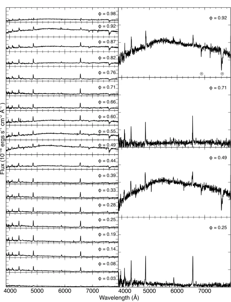
In region 3, the continuum in the high state is broadly in-flated compared to region 2, and to the low state. It does not show any distinct cyclotron humps, but has a maximum in the optical band around 5500 ˚A. This can be seen in Figure 7 which shows a time-series of LSQ1725-64 in the high state. To illustrate theincrease in the continuum dur-ing the high state, the panels on the right show high state spectra with the low state spectra of corresponding phase subtracted. Those labelled φ = 0.49 and 0.92 correspond to maxima in the photometric lightcurve and in the spec-troscopy. By analogy with BL Hydri (Schwope et al. 1995), the extra light we see in the continuum is consistent with a blended set of closely spaced cyclotron harmonics that ap-pear when the accreting pole is in view. We estimate we are seeing harmonics around n = 17 given our measured field
strength of 12.5 MG. Wickramasinghe & Meggitt (1985) show that at high viewing angles to the magnetic field axis, like we have at phases 0.49 and 0.92, most of the cyclotron intensity is concentrated at higher harmonics. Polarization measurements during the high state are required to confirm this view.
In the low state, regions 2 and 3 are more similar to each other, consistent with a dramatic reduction or cessa-tion of accrecessa-tion. We have averaged all the low state spectra to improve the signal-to-noise and yield a spectrum that is relatively uncontaminated by accretion light (Figure 8). The continuum is dominated by the white dwarf photosphere on the blue end and features from the secondary star on the red end. We have excluded region 1 from our average.
Figure 6.Nightly PROMPT monitoring (colours) showing the transition from the low state (top left) to the high state (bottom right). SOAR low and high state lightcurves are repeated in grey for reference. The cycle counts and times correspond to the leftmost side of each figure. We observe the return to highest state to occur over∼45 orbits.
fit the surface gravity of the white dwarf. Instead, we use the best radius and surface gravity derived later from eclipse pa-rameters (subsection 6.2) and the white dwarf mass-radius relation to estimate log(g) ∼ 8.5. We tested different
val-ues of log(g) and found that the white dwarf temperature is relatively insensitive to log(g).
Our best-fitting composite model is shown inFigure 8. The poor fit at the shortest wavelengths is due to poor flux calibration due to extinction and differential slit losses (see section 2). The best-fitting composite model has a white dwarf temperature of 12650±550 K and a secondary
spec-tral type of M8±0.5. The secondary spectral type is
insensi-tive to the uncertainty in the white dwarf temperature. The fitted distances are 326 ±93 pc and 222±112 pc for the
white dwarf and M-dwarf respectively. Taking a weighted av-erage, we estimate the best distance to LSQ1725-64 is 284
±71 pc.
5.2 Emission Line Measurements
The high state spectra show strong Balmer emission lines along with He I throughout every phase except eclipse, while in the low state the Balmer lines are reduced and He I is absent (see Figure 7 and Figure 8). We also detect weak He II (4686 ˚A) in some but not all of our spectra. In a few of our spectra on 2013-07-03, which were made in a setup with a bluer limit, we also detect Ca II at 3933 ˚A. The strength varies significantly with orbital phase and is strongest around phase 0.60. This phasing of the Ca II sug-gests that it also comes from the irradiated photosphere of the secondary, but we do not have enough signal to noise in individual spectra to confirm using radial velocities.
The Polar LSQ1725-64
9
Figure 8.Combined fit to the low state orbital averaged spectrum of LSQ1725-64 (black) with an M8 (red) secondary and 12650 K and log(g) = 8.5 non-magnetic white dwarf (blue). The combined white dwarf + M8 spectrum is shown in green. The black bars at the top show the regions of the spectrum that were used in the fit. We excluded the Balmer lines, emission lines, and telluric absorption.
we are only able to resolve these components at extrema in the stream velocities, so detailed study of the independent components or Doppler Tomography is not possible using our data.
The Balmer decrement can give us some idea of the tem-perature and density of the line emitting region, which in the high state we presume is predominantly from a section of the ballistic accretion stream (see subsubsection 5.2.1). From high state spectra of LSQ1725-64, we measure the ratios
Hα/Hβ = 1.05 and Hγ/Hβ = 0.86.Williams (1991)
cal-culates Balmer ratios in cataclysmic variables over a range of temperatures and densities. The ratios in LSQ1725-64 roughly correspond to gas with temperature of 8000 - 10000 K and log(NH) between 12.5 and 13.5. These values are similar to those found byGerke et al.(2006) for their mea-surement of the Balmer decrement in the streams of other polars.
Just before eclipse, we see an absorption component appear on the blue side of the emission line, forming a P Cygni profile. This is shown inFigure 9, which compares H
αat phases 0.49 and 0.98 in the high and low state. Similar P Cygni profiles also appear in Hβand He I (5876 ˚A) just before eclipse in the high state. None of these lines show absorption or P Cygni profiles in the low state. We show trailed spectra from high and low state in Online Figure 2.
Schmidt et al.(2005) measure P Cygni profiles in multi-ple lines in FL Cet just before eclipse, and following a model fromSchwope et al. (1997) for HU Aquarii, they attribute the absorption to material in an accretion funnel just above the white dwarf. In Hu Aqr, similarly placed material causes
a dip in the photometric light curve, and is described by Schwope et al.(1997) as being in a stagnation region where the infalling stream has attached to the magnetic field and is being redirected along field lines towards a magnetic pole. These field lines may direct the material out of the orbital plane or away from the line of centres, thereby changing the projected velocity. Near eclipse, when the projected stream velocity is at a maximum, the result will be a comparatively lower redshift, and hence the P Cygni profile we observe.
5.2.1 Radial Velocities
We measured radial velocities of H α, H β, H γ, and
He I (5876 ˚A) on four different nights while LSQ1725-64 was in the high state. The emission lines at each orbital phase were fitted with a gaussian. At phases where the lines could not be fitted (mostly around the eclipse) we discarded the results. We used the 5577 ˚A sky line to adjust our wave-length solution for each spectrum. We then fitted the time series for each emission line using the equation
vr=γ+Ksin 2π(φ−φ0), (4) holding the period fixed to that measured insubsection 4.1 so that the fitted parameters are the systemic velocity, radial velocity amplitude, and phase.
We quantitatively confirm the result fromRabinowitz et al. (2011) that the maximum redshift occurs just af-ter phase 0, at phase 0.044± 0.001. This difference is
The Polar LSQ1725-64
11
Figure 9.Comparison of Hαemission at different phases during high and low states. The data have been continuum subtracted using the continuum flux at 6450 ˚A. The accretion stream in the high state overwhelms the contribution from the secondary star near phase 0.5 (seesubsubsection 5.2.1). The presence and absence of the P Cygni profile in high and low state, respectively, is shown near phase 1.
Peters 1972). This reinforces the point that the primary source of emission is along the infalling ballistic accretion stream. The average radial velocity amplitude we measure is 507±18km s−1. The average systemic velocity we
mea-sure is 40±25km s−1. We show this result in the top panel
ofFigure 10.
We show in the bottom panel of Figure 10 the fitted radial velocities of Hαduring a low state. The best-fitting H αcurve from our high state measurements is shown as a solid green curve. The expected radial velocity from the secondary using the parameters in subsection 6.2 is shown as a dashed red curve. In phases centred on white dwarf eclipse (white background), when we see the un-irradiated side of the secondary, the data generally follow the Hαradial velocity curve from the ballistic stream, as in the high state. However, in phases centred on 0.5 (gray background), when emission from the secondary should be at its largest, the data more closely follow the expected orbital radial velocity curve of the secondary star.
The upper panel ofFigure 9compares the reprocessed Hαin the low state with the high state emission from the stream near its maximum blueshift (φ= 0.49). Overall, the fitted radial velocities provide evidence that some of the light is from residual accretion occurring during the low state, but also that reprocessed light from the irradiated secondary is now much more easily measured.
6 DISCUSSION
Our observations have refined and expanded our under-standing of the properties of LSQ1725-64 as first presented by Rabinowitz et al. (2011). In this section, we will dis-cuss three key questions about LSQ1725-64 thatRabinowitz et al. (2011) were either unable to address or able to ad-dress only partially: the evolutionary state of the system, the masses and radii of the stars in the binary, and an esti-mate of the mass transfer rate.
6.1 Is LSQ1725-64 a post-bounce system?
Rabinowitz et al. (2011) suggested LSQ1725-64 is a post-bounce system based on the very red limit they derived for theV-J colour and their fitting of binary parameters. How-ever, their determination suffered from two limitations: their time resolution gave them a crude estimate of the eclipse length, and they did not detect the secondary during eclipse in any band other than J. In this section we will use our better data to argue that LSQ1725-64 has properties most consistent with a pre-bounce system.
6.1.1 Argument based on eclipse length
Using our highest time resolution photometry from SALT, we have measured an eclipse length from ingress to mid-egress of ∆φ= 0.066±0.002, a value for the eclipse length
at the upper end of the range given by Rabinowitz et al. (2011).
With our more precise measurement of eclipse length, we can repeat the procedure ofRabinowitz et al.(2011) to solve four equations for four unknowns using a Monte Carlo method to estimate errors in the parameters. The equations are the period-mean density relationship for Roche lobe fill-ing secondaries (Equation C1), the mass-radius relationship for pre- and post-bounce systems fromKnigge (2006), Ke-pler’s Law (Equation C4), and the relationship between in-clination and eclipse length (Equation C5). Following Rabi-nowitz et al.(2011) we assume in our fit a white dwarf mass of 0.75M⊙and radius of 0.0013 R⊙.
Using a Gaussian distribution of the measured param-eters, we find that only 0.08 per cent of our one million Monte Carlo simulations return a result with a large enough post-bounce secondary to create the eclipse length we mea-sure. Therefore, we consider a post-bounce solution very un-likely. Conversely, using the pre-bounce mass-radius relation (Equation C2) we find the majority of solutions have param-eters close to the values we measure.
6.1.2 Argument based on spectral type
Out best-fitting composite spectrum in subsection 5.1 yielded a spectral type of M8, with an uncertainty of about half a spectral type. This is much earlier than expected for a post-bounce system, as illustrated inFigure 11. The ver-tical bars in that figure mark the masses of secondaries on the pre-bounce (red) and post-bounce (green) sequence of Knigge (2006). Our best spectral fit lies within the scatter of the pbounce masses. A post-bounce solution would re-quire a spectrum in the late T range, which is firmly ruled out by our spectrum.
Figure 11. Constraints on the spectral type and mass of the secondary in LSQ1725-64. The green vertical line shows the post-bounce secondary mass from the models ofKnigge(2006). The red vertical line and shaded region shows the pre-bounce secondary mass and distribution fromKnigge(2006). We show three differ-ent constraints on the secondary mass, arising from flux measure-ments of the secondary. The lowest constraint is from our spectral decomposition, the middle constraint is from ourR-Jcolour, and the top constraint is from theV-Jlimit measured byRabinowitz et al.(2011). Our results are more consistent with LSQ1725-64 being a pre-bounce system.
The V-J limit of Rabinowitz et al. (2011), shown at the top of Figure 11, is just consistent with our spectral type. We also detected LSQ1725-64 in a limited number of our photometric observations in ther′ andi′ bands. Using the transformation of Lupton (2005)1
, we converted these into anR-band magnitude, and combined them with the J-band measurement ofRabinowitz et al.(2011) to get anR-J colour of 4.9±0.4. This result also supports identification
of LSQ1725-64 as a pre-bounce system.
From all of the evidence available, it appears that the secondary in LSQ1725-64 is too large, and too early in spec-tral type for LSQ1725-64 to be a post-bounce system.
6.2 Binary Parameters
Because we have measured the eclipse egress length with pre-cision, we can derive new binary parameters of LSQ1725-64 using a set of six equations instead of the four that Ra-binowitz et al. (2011) used. We give the six equations in Appendix C.
We solved the equations Monte Carlo style to esti-mate the binary parameters with errors, treating each mea-sured value and error as a Gaussian distribution. Our in-puts included the measured mid-egress time of φegress = 0.033±0.001 and our measured length of the white dwarf
egress of tegress = 23.4 ± 0.3 s, along with the orbital period. We ran one million simulations and rejected solu-tions that did not have secondaries large enough to match
1
The Polar LSQ1725-64
13
the eclipse length. Our output results and the associated 1σ
errors are shown inTable 3.
Our white dwarf mass of 0.97±0.03 M⊙ falls within
the white dwarf mass distribution in cataclysmic variables ofZorotovic et al.(2011). This value also is similar to other known white dwarf masses in polars (e.g. Cropper et al. (1998)) though the number of polars with directly measured white dwarf masses is still small. Adopting different white dwarf mass-radius relationships from Panei et al. (2000) for different core compositions changes our results insignif-icantly, except for an iron-core white dwarf, which is not something we expect. Thus LSQ1725-64 provides another indication that the white dwarfs in cataclysmic variables are significantly more massive than those of typical single white dwarfs, whose masses cluster in a narrow range around 0.63
M⊙(Falcon et al. 2010).
6.3 Mass Transfer Rate
Normally, the mass transfer rate in polars is measured through the accretion luminosity in the X-ray or UV com-bined with a distance (see e.g. King & Watson (1987)). Then, if the magnetic field is known, an estimate of the Alfv´en radius,rµ, can also be calculated. This approach is beyond the scope of this paper, but we can make a rough estimate of the mass transfer rate from calculating the lower limit ofrµ.
Bridge et al. (2003) used the eclipse of the accretion stream they measured in EP Dra to estimate the Alfv´en radius. We can use the eclipse of the accretion stream seen inFigure 3in the same way to get an estimate ofrµ. As with EP Dra, this stream is variable as is the mass transfer rate, but will provide an estimate for rµ. The stream subtends an orbital phase of ∆φ= 0.025±0.002. We converted this
into a projected length using the measured accretion spot longitude of 99 degrees and a co-latitude ofβ= 90 to get a lower limit on the Alfv´en radius of 0.120±0.009R⊙.
UsingMukai(1988) andWarner(1995):
˙
M16=
1.45×10¹⁰
rµ
11/2
µ234 σ
2 9 M
−1/2
wd (5)
we can convert this into an estimate of the upper limit of ˙
M16. The resulting upper limit is 3.8±2.1×10¹⁵g s−1 or 6.1±3.4×10⁻¹¹M⊙ yr−1, where we have used the stream
radius, σ9, from Lubow & Shu (1975) for the appropriate mass ratio and assumed a dipole field.
There are a number of assumptions and simplifications that are involved in this estimate. X-ray or UV measure-ments of LSQ1725-64 are required to provide a measurement of the mass transfer rate. However, our estimate is within the range of mass transfer rates seen in other polars (Warner 1995), and similar to those derived byAraujo-Betancor et al. (2005) andTownsley & G¨ansicke(2009) for polars with or-bital periods like LSQ1725-64.
This can be compared with the expected ˙M from grav-itational radiation alone. FromWarner(1995)
˙
M = 2.4×10¹⁵ M
2/3 wdP
−1/6 orb (hr)
1−15 19q
(1 +q)1/3
g s−1
, (6)
which gives a predicted mass transfer rate of ∼ 2.3×
1015
g s−1
. Our estimated limit on the mass transfer rate
is consistent with this expectation from gravitational radi-ation, and does not require any extra source of braking to explain. This result is consistent with the overall picture of polar evolution (e.g.Wickramasinghe & Wu(1994)).
7 CONCLUSIONS
We have presented new observations of the short period (94 m) eclipsing binary LSQ172554.8-643839 that confirm it is a magnetic cataclysmic variable of the AM Herculis type. Photometric monitoring with the SOAR Telescope, SALT, and PROMPT has revealed high states separated by∼109
days with 65 per cent duty cycle, indicative of changes in the mass-transfer state. The transition from low to high state occurs over a three day period, or about 45 orbits. Strong emission lines present during the high state show properties consistent with emission from a bright accretion stream. The stream emission lines fade in intensity during the low state, but do not disappear, indicating that mass transfer contin-ues throughout the accretion cycle.
Using the Zeeman splitting of the Hβ absorption line of the white dwarf, we have estimated the surface-averaged magnetic field to be 12.5±0.5 MG. We have fitted the
av-erage low state spectrum to yield an estimate of the white dwarf temperature (12650±550K) and secondary spectral
type (M8±0.5). Based on the spectral type and the eclipse
length, we have established that LSQ1725-64 is in the pre-bounce evolutionary phase.
Our time-resolved photometry and spectroscopy has permitted us to make precise estimates of system parame-ters, including the white dwarf radius (0.0085±0.0003R⊙),
which implies a mass of 0.97±0.03 M⊙. If we identify the
height of the gas above the limb as an estimate of the Alfv´en radius, we estimate an upper limit to the average mass trans-fer rate of 6.1±3.4×10⁻¹¹M⊙yr−1. This result is consistent
with expectations from angular momentum loss via gravita-tional radiation alone.
Among polars, LSQ1725-64 is an ideal laboratory in many respects. The geometry is simple and measurable, dif-ferent accretion states are frequent and dramatic, and the accretion on to one pole leaves a ‘reference hemisphere’ on the white dwarf in the high state. There have been bothSwift andXMM-Newton observations of LSQ1725-64. Analyzing these data is beyond the scope of this paper, but investi-gating these observations will help measure the accretion luminosity and infer a mass transfer rate. Additional multi-wavelength studies, polarization measurements, and detailed modeling of the system should illuminate many outstanding questions about the origin and evolution of this polar, and the nature of its accretion states.
ACKNOWLEDGEMENTS
Table 3.Binary Parameters of LSQ1725-64
φegress Mwd(M⊙) Rwd(R⊙) M2(M⊙) R2(R⊙) a (R⊙) i(degrees)
0.033±0.001 0.966±0.027 0.0085±0.0003 0.114±0.021 0.155±0.010 0.703±0.010 85.6±1.7
from the National Science Foundation, under award AST-1413001. J.T.F. thanks the taxpayers of North Carolina for their support as a Teaching Assistant. Some of the observa-tions reported in this paper were obtained with the Southern African Large Telescope (SALT) under program 2013-1-UNC-RSA-002 (PI: Fuchs). Figures were made with Veusz, a free scientific plotting package written by Jeremy Sanders. Veusz can be found at http://home.gna.org/veusz/. The white dwarf cooling models used can be found at
http://www.astro.umontreal.ca/~bergeron/CoolingModels. This research was made possible through the use of the AAVSO Photometric All-SkySurvy (APASS), funded by the Robert Martin Ayers Sciences Fund.
REFERENCES
Araujo-Betancor S., G¨ansicke B. T., Long K. S., Beuer-mann K., de Martino D., Sion E. M., Szkody P., 2005, ApJ, 622, 589 [6.3]
Beuermann K., Euchner F., Reinsch K., Jordan S., G¨ansicke B. T., 2007,A&A, 463, 647 [1]
Beuermann K., Thomas H. C., Giommi P., Tagliaferri G., 1987,A&A, 175, L9 [4.2.1]
Bochanski J. J., West A. A., Hawley S. L., Covey K. R., 2007,AJ, 133, 531 [5.1]
Bridge C. M., Cropper M., Ramsay G., de Bruijne J. H. J., Reynolds A. P., Perryman M. A. C., 2003,MNRAS, 341, 863 [4.2.1,6.3]
Claret A., Bloemen S., 2011,A&A, 529, A75 [B]
Clemens J. C., Crain J. A., Anderson R., 2004, in Moor-wood A. F. M., Iye M., eds, Ground-based Instrumenta-tion for Astronomy Vol. 5492 of Society of Photo-Optical Instrumentation Engineers (SPIE) Conference Series, The Goodman spectrograph. pp 331–340 [2]
Cropper M., 1990, SSR, 54, 195 [1]
Cropper M., Mason K., Allington-Smith J., Branduardi-Raymont G., Charles P., Mittaz J., Mukai K., Murdin P., Smale A., 1989, MNRAS, 236, 29 [1]
Cropper M., Ramsay G., Wu K., 1998,MNRAS, 293, 222 [6.2]
Eastman J., Siverd R., Gaudi B., 2010, PASP, 122, 935 [4.1]
Eggleton P., 1983, ApJ, 268, 368 [B]
Falcon R. E., Winget D. E., Montgomery M. H., Williams K. A., 2010,ApJ, 712, 585 [6.2]
G¨ansicke B. T., Dillon M., Southworth J., Thorstensen J. R., Rodr´ıguez-Gil P., Aungwerojwit A., Marsh T. R., Szkody P., Barros S. C. C., Casares J., de Martino D., Groot P. J., Hakala P., Kolb U., Littlefair S. P., 2009, MNRAS, 397, 2170 [1]
Gerke J. R., Howell S. B., Walter F. M., 2006,PASP, 118, 678 [4.3,5.2]
Hessman F., G¨ansicke B. T., Mattei J., 2000, A&A, 361, 952 [1]
Holberg J. B., Bergeron P., 2006,AJ, 132, 1221 [(iii)] Horne K., Gomer R. H., Lanning H. H., 1982, ApJ, 252,
681 [(v)]
King A. R., Cannizzo J. K., 1998,ApJ, 499, 348 [4.3] King A. R., Watson M. G., 1987,MNRAS, 227, 205 [6.3] Knigge C., 2006,MNRAS, 373, 484 [6.1.1,6.1.2,11,(ii)] Koester D., 2010,Mem. Soc. Astron. Ital., 81, 921 [5.1] Kopal Z., ed. 1978, Dynamics of close binary systems
Vol. 68 of Astrophysics and Space Science Library [B, B]
Landstreet J. D., 1980,AJ, 85, 611 [3]
Littlefair S. P., Dhillon V. S., Marsh T. R., G¨ansicke B. T., Southworth J., Watson C. A., 2006, Science, 314, 1578 [1] Lubow S. H., Shu F. H., 1975,ApJ, 198, 383 [6.3] Markwardt C., 2009, in Bohlender D., Durand D., Dowler
P., eds, Astronomical Data Analysis Software and Systems XVIII Vol. 411 of Astronomical Society of the Pacific Con-ference Series, Non-linear least-squares fitting in idl with mpfit. p. 251 [4.1]
Morris S., Naftilan S., 1993, ApJ, 419, 344 [B] Mukai K., 1988,MNRAS, 232, 175 [6.3]
Nucita A. A., De Paolis F., Ingrosso G., 2012, Journal of Physics Conference Series, 354, 012013 [(vi)]
O’Donoghue D., Buckley D. A. H., Balona L. A., Bester D., Botha L., Brink J., Carter D. B., Charles P. A., Chris-tians A., Ebrahim F., Emmerich R., Esterhuyse W., Evans G. P., Fourie C., Fourie P., Gajjar H., Gordon M., Gumede C., de Kock M., Koeslag A., Koorts W. P., 2006, MNRAS, 372, 151 [2,4.2.1]
Panei J. A., Althaus L. G., Benvenuto O. G., 2000,A&A, 353, 970 [6.2]
Patterson J., 1984,ApJS, 54, 443 [1]
Piro A. L., Arras P., Bildsten L., 2005,ApJ, 628, 401 [4.2.2] Rabinowitz D., Tourtellotte S., Rojo P., Hoyer S., Folatelli G., Coppi P., Baltay C., Bailyn C., 2011,ApJ, 732, 51 [1, 4.2.1,3,5.2.1,6,6.1,6.1.1,11,6.1.2,6.2]
Ramsay G., Cropper M., Wu K., Mason K., Cordova F., Priedhorsky W., 2004, MNRAS, 350, 1373 [5.2]
Rebassa-Mansergas A., G¨ansicke B. T., Rodr´ıguez-Gil P., Schreiber M. R., Koester D., 2007, MNRAS, 382, 1377 [5.1]
Rosen S. R., Mittaz J. P. D., Buckley D. A., Layden A. C., Clayton K. L., McCain C., Wynn G. A., Sirk M. M., Osborne J. P., Watson M. G., 1996, MNRAS, 280, 1121 [4.2.2]
Schmidt G. D., Szkody P., Homer L., Smith P. S., Chen B., Henden A., Solheim J.-E., Wolfe M. A., Greimel R., 2005,ApJ, 620, 422 [5.2]
Schwarz R., Greiner J., Tovmassian G. H., Zharikov S. V., Wenzel W., 2002,A&A, 392, 505 [4.2.2]
Schwope A. D., Beuermann K., Jordan S., 1995,A&A, 301, 447 [5.1]
Schwope A. D., Mantel K.-H., Horne K., 1997,A&A, 319, 894 [5.2]
The Polar LSQ1725-64
15
Szkody P., 1998, in Howell S., Kuulkers E., Woodward C., eds, Wild Stars in the Old West Vol. 137 of Astronomi-cal Society of the Pacific Conference Series, Spectroscopy of Cataclysmic Variables: Whopping Clues from Wiggly Lines. p. 18 [1]
Townsley D., G¨ansicke B. T., 2009, The Astrophysical Journal, 693, 1007 [4.2.2,6.3]
Tremblay P.-E., Bergeron P., Gianninas A., 2011,ApJ, 730, 128 [(iii)]
Warner B., 1995, Cambridge Astrophysics Series, 28 [1, 6.3,6.3,(v)]
Warner B., 1999, in Hellier C., Mukai K., eds, Annapolis Workshop on Magnetic Cataclysmic Variables Vol. 157 of Astronomical Society of the Pacific Conference Series, Low States in Cataclysmic Variables. p. 63 [1]
Warner B., Peters W. L., 1972,MNRAS, 160, 15 [5.2.1] Wheatley P. J., Ramsay G., 1998, ASPC, 137, 446 [1] Wheatley P. J., West R. G., 2002, in G¨ansicke B. T.,
Beuer-mann K., Reinsch K., eds, The Physics of Cataclysmic Variables and Related Objects Vol. 261 of Astronomical Society of the Pacific Conference Series, Further analy-sis of the X-ray eclipse of OY Car measured with XMM-Newton. p. 433 [(vi)]
Wickramasinghe D. T., Ferrario L., 2000, PASP, 112, 873 [1]
Wickramasinghe D. T., Meggitt S. M. A., 1985,MNRAS, 214, 605 [5.1]
Wickramasinghe D. T., Wu K., 1994,MNRAS, 266, L1 [6.3] Williams G. A., 1991,AJ, 101, 1929 [5.2]
Wu K., Kiss L., 2008,A&A, 481, 433 [4.3]
Zorotovic M., Schreiber M. R., G¨ansicke B. T., 2011,A&A, 536, A42 [6.2]
APPENDIX A: ECLIPSE TIMINGS
We include all eclipse timings used to update the ephemeris inTable A1.
APPENDIX B: ELLIPSOIDAL MODULATIONS AS A FUNCTION OF MASS RATIO
Here we compute the theoretical dependence of ellipsoidal variation amplitude as a function of the mass ratio, q =
Msec
Mwd.
A description of ellipsoidal variability can be found in Kopal(1978). This has been summarized nicely byMorris & Naftilan(1993), who expanded the periodic variations into a discrete Fourier series. The fifth term from Equation 1 of Morris & Naftilan (1993) gives the expected amplitude of the ellipsoidal variation for a Roche Lobe filling star. We ignore terms that are of order (R/a)4 and higher to yield fractional amplitudes as
∆F
Fsec
= 0.15(15 +u)(1 +τ) (3−u)
1
q
Rsec
a
3
sin2i, (B1) where u is the limb darkening coefficient, τ is the gravity darkening coefficient, Rsec is the radius of the secondary star, ais the orbital separation, and iis the inclination of the system. Based on our characterization of the secondary insubsubsection 6.1.2andClaret & Bloemen(2011) we use
Figure B1.The expected fractional amplitude of ellipsoidal vari-ations of a Roche lobe filling secondary as a function of mass ratio. The red triangle shows that the maximum expected fractional flux change for the mass ratio of LSQ1725-64 (subsection 6.2is only 11.7 per cent. Thus, the 50 per cent inferred photometric varia-tion shown inFigure 4is too large to be explained by ellipsoidal variations alone.
u= 0.6 andτ = 0.4. Employing our best-fitting inclination of 85.6 degrees (subsection 6.2) this becomes
0.15(15 +u)(1 +τ) (3−u) sin
2
i = 1.36. (B2)
We can then write the fractional amplitude as
∆F
Fsec
=1.36
q
Rsec
a
3
. (B3)
Furthermore, Eggleton (1983) gives an approximation to the Roche radius as
Rsec
a =
0.49q2/3
0.6q2/3+ ln (1 +q1/3) , (B4) which is accurate to within 1 per cent of the tabulation by Kopal(1978). This allows us to write the expected fractional amplitude as a function of the mass ratio
∆F
Fsec
=1.36
q
0.49q2/3 0.6q2/3+ ln (1 +q1/3)
3
. (B5)
Table A1.Eclipse timings used to update the ephemeris.
Observation Date Instrument Exposure Time (s) Mid-egress Time Mid-egress Time O-C (s)
Start (UT) (BJ DT DB) Error (10−5 days)
2011-09-07 SALTICAM 15.7 2455812.309128 12.3 2.30
2012-08-12 Goodman 20 2456152.522472 2.5 -3.01
2012-08-12 Goodman 20 2456152.588247 1.2 -0.15
2013-06-08 Goodman 20 2456451.713065 10.7 -1.19
2013-06-08 Goodman 20 2456451.778822 7.6 0.14
2013-07-03 Goodman 20 2456476.563494 2.3 3.79
2013-07-03 Goodman 20 2456476.629218 1.6 2.33
2013-07-06 SALTICAM 1.7 2456480.442182 5.7 -2.51
2013-07-12 Goodman 12 2456486.490430 3.1 -1.65
2013-07-12 Goodman 12 2456486.556206 1.6 1.27
2013-08-05 Goodman 12 2456510.486178 2.0 0.07
2013-08-05 Goodman 12 2456510.551916 2.4 -0.28
2013-08-14 Goodman 11 2456519.492761 2.8 -2.79
2013-08-14 Goodman 11 2456519.558514 2.1 -1.85
2013-08-15 Goodman 12 2456520.478891 8.2 -2.40
2013-09-02 SALTICAM 1.7 2456538.294926 1.2 0.02
2013-11-14 Goodman 12 2456610.545059 4.2 -1.58
2014-06-30 Goodman 12 2456838.603099 4.2 -0.65
2014-06-30 Goodman 12 2456838.668777 4.3 -6.23
APPENDIX C: EQUATIONS FOR BINARY PARAMETER CALCULATION
The six equations we use to solve the binary parameters of LSQ1725-64 are:
(i) The Roche condition:
R2
R⊙
= 0.2361Porb,h2/3 M2
M⊙
1/3
, (C1)
wherePorb,his the orbital period in hours.
(ii) The mass-radius relation of cataclysmic variable sec-ondaries for the pre-bounce sequence ofKnigge(2006):
R2
R⊙
= 0.230±0.008 M2
0.20±0.02M⊙
0.64±0.02
(C2)
(iii) The mass-radius relationship for white dwarfs from a polynomial fit to the cooling models ofHolberg & Bergeron (2006) andTremblay et al.(2011)2
, which assume a CO core white dwarf:
Rwd=−0.009297M 3
wd+0.02669Mwd2 −0.03678Mwd+0.02747. (C3) (iv) Kepler’s Law:
a3=Porb2 Mwd+M2
G 4π2
(C4)
(v) The relationship between the inclination, secondary radius, separation, and eclipse length given by Warner (1995) andHorne et al.(1982):
sin2
(i)≈ 1−(R2/a)
2
cos2(2π φegress) , (C5) whereφegressis the phase of mid-egress andφ= 0 is inferior conjunction of the secondary.
2
see http://www.astro.umontreal.ca/ bergeron/CoolingModels/
(vi) The length of the white dwarf egress, which depends on the path the white dwarf takes behind the secondary (see Wheatley & West(2002) andNucita et al.(2012)):
tegress
Porb
=
p
[R2+Rwd]2−[acos(i)]2− p
[R2−Rwd]2−[acos(i)]2 2πa