The SAMI Galaxy Survey: Asymmetry in Gas Kinematics
and its links to Stellar Mass and Star Formation
J. V. Bloom
1,2?, L. M. R. Fogarty
1,2, S. M. Croom
1,2, A. Schaefer
1,2, J. J. Bryant
1,2,3,
L. Cortese
4, S. Richards
1,2,3, J. Bland-Hawthorn
1, I-T. Ho
6, N. Scott
1,2, G. Goldstein
7,
A. Medling
8, S. Brough
3, S.M. Sweet
8, G. Cecil
9, A. L´
opez-S´
anchez
3,7, K. Glazebrook
3,
Q. Parker
10,3,7, J. T. Allen
1,2, M. Goodwin
3, A. W. Green
3,
I. S. Konstantopoulos
3,11, J. S. Lawrence
3, N. Lorente
3, M. S. Owers
3,7, R. Sharp
8 1 Sydney Institute for Astronomy, School of Physics, University of Sydney, NSW 2006, Australia.2 ARC Centre of Excellence for All-Sky Astrophysics (CAASTRO).
3 Australian Astronomical Observatory, PO Box 915, North Ryde, NSW 1670, Australia.
4 International Centre for Radio Astronomy Research, The University of Western Australia, 35 Stirling Hwy, Crawley, WA 6009, Australia 5 Centre for Astrophysics and Supercomputing, Swinburne University of Technology, Hawthorn, VIC 3122, Australia.
6 Institute for Astronomy, University of Hawaii, 2680 Woodlawn Drive, Honolulu, HI 96822, USA. 7 Dept. Physics and Astronomy, Macquarie University, NSW 2109, Australia
8 Research School for Astronomy & Astrophysics. Mount Stromlo Observatory, ANU, Cotter Road Weston Creek, ACT 2611 Australia. 9 Dept. Physics and Astronomy University of North Carolina Chapel Hill, NC 27599 USA
10Department of Physics, The University of Hong Kong, Hong Kong
11Envizi Group Suite 213, National Innovation Centre, Australian Technology Park, 4 Cornwallis Street, Eveleigh NSW 2015, Australia
25 September 2018
ABSTRACT
We study the properties of kinematically disturbed galaxies in the SAMI Galaxy Survey using a quantitative criterion, based on kinemetry (Krajnovi´c et al.). The approach, similar to the application of kinemetry by Shapiro et al. uses ionised gas kinematics, probed by Hα emission. By this method 23±7% of our 360-galaxy sub-sample of the SAMI Galaxy Survey are kinematically asymmetric. Visual classifica-tions agree with our kinemetric results for 90% of asymmetric and 95% of normal galaxies. We find stellar mass and kinematic asymmetry are inversely correlated and that kinematic asymmetry is both more frequent and stronger in low-mass galaxies. This builds on previous studies that found high fractions of kinematic asymmetry in low mass galaxies using a variety of different methods. Concentration of star forma-tion and kinematic disturbance are found to be correlated, confirming results found in previous work. This effect is stronger for high mass galaxies (log(M∗)>10) and
in-dicates that kinematic disturbance is linked to centrally concentrated star formation. Comparison of the inner (within 0.5Re) and outer Hαequivalent widths of asymmetric and normal galaxies shows a small but significant increase in inner equivalent width for asymmetric galaxies.
Key words: galaxies: evolution galaxies: kinematics and dynamics galaxies: structure galaxies: interactions - techniques: imaging spectroscopy - methods: data analysis
1 INTRODUCTION
Hierarchical galaxy formation, in which dark matter halos form through a series of mergers, is central to ΛCDM cos-mology (Peebles 1982; Cole et al. 2008; Neistein & Dekel 2008). It is well-established from N-body simulations [e.g.
Mayer et al.(2007); Stewart et al.(2009)] that the rate of
both halo and galaxy mergers should vary with redshift, but the precise details are not yet fully understood. There are discrepancies between theory and observation. For example, major mergers are known from theory to transform disky galaxies into thick, flared, bulge-dominated systems, that we would then expect to dominate the local universe. We
c
instead see a large proportion of thin, disky systems at low redshift (Mihos & Hernquist 1994;Zucca et al. 2006).
Previous studies of galaxy disturbance have used im-ages to either visually or quantitatively calculate the degree of disturbance within galaxies [e.g.Burkey et al.(1994);Lotz
et al. (2004); De Propris et al.(2007); Darg et al.(2010)].
Visual identification of close pairs was used to determine merger rates in the Sloan Digital Sky Survey (SDSS) (
Elli-son et al. 2013) and Galaxy And Mass Assembly (GAMA)
Survey (Robotham et al. 2014) samples. Structural analy-sis has also been used (Casteels et al. 2014). These methods have been employed to determine merger rates in the nearby
(Darg et al. 2010) and high redshift (Conselice et al. 2003a)
universe. These merger rates are, however, not always con-sistent. For example, the merger rate calculated by close pair counting inLin et al.(2004) is an order of magnitude lower than that found byConselice et al.(2003a). The discrepancy has been noted in the literature, and efforts have been made to reconcile different results from different methods, such as
inLotz et al.(2011).
Despite the success of these approaches, they have lim-itations: purely visual analyses are difficult (although not impossible) to quantify (Casteels et al. 2013), and quanti-tative morphological techniques can be influenced by Hub-ble type and are restricted in the range of asymmetries to which they are sensitive. This is the case in the Con-centration/Asymmetry/Smoothness system (Conselice et al.
2003b). The Asymmetry parameter can be influenced by the
presence of spiral arms, which can mask the effects of mi-nor asymmetries (Conselice et al. 2003b). Further, at high redshift, galaxies may be photometrically asymmetric but kinematically regular, due to features such as clumpy star formation (Glazebrook 2012).
Recent technological advances have revolutionised the reach of spectroscopy. Previously, the majority of spectro-scopic measurements were taken with a single fibre or slit [e.g.York et al.(2000); Percival et al.(2001);Driver et al.
(2009)]. For extended sources, such as galaxies, this ap-proach is highly vulnerable to aperture effects, and it is diffi-cult to gather information about spatial variation across the source. Integral field spectroscopy (IFS) solves this prob-lem by taking spectra at various positions across the object, opening up new scientific possibilities.
Instruments such as KMOS (Sharples et al. 2013), FLAMES (Pasquini et al. 2002) and SINFONI (Eisenhauer
et al. 2003) have demonstrated the usefulness of IFS. Surveys
such as SINS (Shapiro et al. 2008) and ATLAS3D(
Cappel-lari et al. 2011) have used IFS technology to spatially
re-solve and measure disturbances in the kinematics of high and low redshift galaxies, respectively. The ATLAS3D and SINS surveys differ in redshift and scale, but they have both demonstrated that the 2D kinematics of galaxies can be used to effectively classify disturbed galaxies at various epochs
(Shapiro et al. 2008). Both SINS and ATLAS3Dused
mono-lithic instruments, which involve taking IFS measurements for each object individually.
The Sydney–AAO Multi-object IFS (SAMI) is a multi-plexed spectrograph, able to produce sample sizes into the thousands of galaxies on a much shorter timescale than a single IFS instrument (Croom et al. 2012). We here demon-strate how the large sample of IFS data in the SAMI Galaxy Survey can be used to determine an asymmetric fraction
(i.e. fraction of galaxies classified as asymmetric) from gas kinematics, using a method based on kinemetry. Further, we show that classification methods based on kinematics are more robust in distinguishing interacting galaxies within the SAMI Galaxy Survey sample than methods based on quan-titative morphology. We finally present results showing links between kinematic asymmetry, concentration of star forma-tion and stellar mass.
In Section2, we give a brief overview of the SAMI in-strument and SAMI Galaxy Survey sample, outlining the data reduction pipeline and production of emission line maps, as well as characterising the sub-sample used in this work. In Section3 we describe the kinematic classification method used to identify kinematically asymmetric galaxies, as well as a visual classification scheme used to calibrate the results from kinemetry. Section 4 shows the results of us-ing kinemetry to identify perturbed galaxies, and compares them directly with results from quantitative morphology. Section5contains a comparison of our results to those from high redshift studies. Sections 6 and 7 show relationships between kinematic asymmetry, stellar mass and star forma-tion rate. Secforma-tion8briefly discusses the AGN in our sample. We conclude in Section9.
2 THE SAMI GALAXY SURVEY
The SAMI Galaxy Survey will consist of 3400 galaxies across a range of stellar masses and environments, within 0.004< z < 0.095 (Croom et al. 2012). The increased size of the survey sample is possible within a relatively short time frame because the SAMI instrument can take observations of up to 12 galaxies at a time (plus one calibration star), greatly increasing the ease with which large samples of IFS data can be obtained.
2.1 The Sydney AAO Multi-object Integral Field Spectrograph
2.2 Sample Selection and Data Reduction
The 3400 galaxies of the SAMI Galaxy Survey were selected from the GAMA survey (Driver et al. 2009), supplemented by 8 galaxy clusters. The GAMA galaxies selected consist of both group and field galaxies, and were chosen to reflect a broad range in stellar mass, in accordance with the science drivers of the SAMI Galaxy Survey. The GAMA galaxies lie on the celestial equator at RA∼9, 12 and 15 hours, covering a total of 144 square degrees. The GAMA survey provides a uniform and highly complete (∼99%),r-band flux limited survey of three large representative regions of the sky (Liske
et al. 2015).
From the GAMA survey galaxies, those with unreliable redshifts or magnitudes were rejected. The final sample con-sists of four stellar mass, volume-limited sub-samples, along with additional dwarf galaxies at low redshift (Bryant et al.
2015).
In order to provide more complete spatial coverage, each galaxy in the sample is observed in a series of 7 exposures. The individual exposures are combined to produce two dat-acubes per galaxy, one for each arm of the spectrograph, with 0.5 arcsec spatial pixels (spaxels).
All reduction of data taken using the AAOmega spec-trograph at the AAT uses the software2dfdr1. The2dfdr package conducts all steps of the data reduction up to the production of wavelength calibration and sky subtracted spectra (Sharp et al. 2015).
The first stage of data reduction using2dfdris the sub-traction of bias and dark frames. In order to ensure good ex-traction of spectra from the 2D data frame, it is necessary to accurately map the positions and profiles of the fibres across the detectors. This is accomplished using a fibre flat field frame, which is taken using an illumination of a white spot on the inside of the AAT dome. Wavelength calibration is then performed, using frames of standard CuAr arc-lamp exposures. Twilight exposures are used to measure the rela-tive throughput between all fibres in the instrument. Finally, there are 26 dedicated sky fibres in the SAMI instrument. These fibres are set to blank sky positions for each field, to measure the sky spectrum, that can then be subtracted from all spectra.
The next steps of the data reduction process, the flux calibration correction and correction for telluric absorption, are independent of 2dfdr, and are conducted using an ex-ternal software suite, written in Python (Allen et al. 2014). For the flux calibration, spectrophotometric standard stars are observed, when possible, on the same night as the galaxy observations. Secondary standard stars are observed simul-taneously with the galaxies, and are used to derive a correc-tion in the telluric bands at 6850–6960˚A and 7130–7360˚A. Datacubes are produced with regular 0”.5 square spaxels. Some spatial resolution is lost when convolving 1”.6 fibres with 0”.5 spaxels, because the flux in each output spaxel is taken as the mean of the flux in each input fibre, with weightings given by the fractional overlap of the fibre with the spaxel. To regain some of the lost resolution, a 0”.8 di-ameter fibre footprint is used to calculate the overlaps, a
drizzle-like process that was initially developed to resam-ple high-resolution imaging fromHST/WPFC2Fruchter &
1 http://www.aao.gov.au/science/software/2dfdr
Hook(2002). The final product is a pair of datacubes per galaxy, one for each arm of the spectrograph, with multiple extensions. The extensions contain, respectively, the flux, variance, weight and covariance datacubes. A full explana-tion of the data reducexplana-tion process can be found in Sharp
et al.(2015)
Due to the re-sampling process used to make the dat-acubes, the noise in neighbouring spaxels is correlated. This effect is negligible for spaxels spaced more than∼2.5 spax-els apart. A full explanation of how covariance is handled in SAMI Galaxy Survey data can be found inSharp et al.
(2015).
2.3 LZIFUand Data Products
LZIFUis an Interactive Data Language (IDL) spectral fitting pipeline, designed to perform flexible emission line fitting in IFS data cubes. It works by fitting, and then removing, the continuum emission in each spaxel by using simple stel-lar population (SSP) models (Ho et al., in prep; Ho et al. 2014).LZIFUuses the penalized pixel-fitting routine,pPXF
(Cappellari & Emsellem 2004) to do the continuum fit. We
use theoretical SSP models, assuming Padova isochrones, of solar metallicity and 18 ages (Delgado et al. 2005). After the continuum emission is removed,LZIFUmodels user-assigned emission lines as Gaussian profiles, and then performs a bounded value nonlinear least-squares fit. This is done us-ingIDL’s Levenberg-Marquardt least-squares method
Mark-wardt (2009), with LZIFU automatically establishing
rea-sonable initial guesses for the wavelength of emission lines. Users have the choice to model individual emission line as either 1, 2, or 3-component Gaussians, describing possible different kinematic components. We use 1-component fits in this work.
The key data products from theLZIFUpipeline are 2D emission line strength and kinematic maps (showing the kinematics of gas in the galaxy, both velocity and veloc-ity dispersion), for user-assigned lines, with error maps. For a more detailed explanation of theLZIFUpipeline, see Ho
et al.(2014).
2.4 Selecting and Characterising the Sample
This work uses the first 451 galaxies to be processed through theLZIFUpipeline. We took the velocity and velocity disper-sion maps generated by the Hαfit fromLZIFUand applied a S/N cut of 10 to the Hαemission map. If, after applying the cut, there were fewer than 200 spaxels remaining in the flux map, out of an original∼1225 spaxels, the galaxy was excluded from the sample (the average being ∼450 spax-els remaining). This was to avoid problems fitting severely discontinuous, low S/N maps. After the above cuts were per-formed there remained a sample of 360 galaxies, which forms the basis of our study.
Fig.1shows the distribution of the rest frame (u−r) colour-stellar mass for our sample (black points) the full SAMI Galaxy Survey sample (blue points), and the par-ent GAMA survey sample (log-spaced red contours). For ease of comparison, the GAMA survey sample in these fig-ures has been restricted to z ≤ 0.095. Likewise, Fig. 2
shows dust obscuration-corrected star formation rate (SFR)
7 8 9 10 11 12
log
(M
∗)0.5 1.0 1.5 2.0 2.5 3.0
Colour (u-r) (mag)
Figure 1.We show colour and stellar mass for the entire GAMA Survey sample (log-spaced red contours) SAMI Galaxy Survey sample (blue points) and the sample used in this work (black dots). Our sample is evenly distributed within the main SAMI Galaxy Survey sample. The data used were taken from the GAMA Data Release 2 catalogues ApMatchedPhotom (Hill et al. 2011) and StellarMasses (Taylor et al. 2011).
Sample log(M∗) (u−r) Colour log(SFR)
SAMI Galaxy
Survey sample 10.04±0.024 1.77±0.012 -0.66±0.023 Our sample 9.70±0.056 1.53±0.028 -0.51±0.053 2KS testp-value 6.15×10⁻⁶ 2.70×10⁻¹⁰ 0.021 Table 1. This table shows the median stellar mass, colour and SFR values for the SAMI Galaxy Survey sample and the sub-sample used in this work, and the results of two-sample Kolmogorov-Smirnov tests for colour, mass and SFR. There is a slight bias towards blue, high-SFR, low stellar mass galaxies in our sample, as is to be expected after performing an HαS/N cut. We nevertheless cover the full parameter space (see Fig.1,2,3). The uncertainty we quote in the table is the statistical error on the median, rather than the uncertainty on SFR or colour for individual galaxies.
against stellar mass, and Fig.3shows redshift against stellar mass, with the GAMA Survey sample in grey. Finally, Fig.4
and Fig. 5show histograms of the colour and specific star formation rate (SSFR) for both samples. SFRs are calcu-lated from the luminosity of the hydrogen Balmer lines. This is because the Balmer emission-line luminosity is directly proportional to the total ionizing flux of the stars in HII re-gions of star forming galaxies. Medians for the stellar mass, colour and SFR for the full SAMI Galaxy Survey Sample and our sample,and the results of two-sample Kolmogorov-Smirnov tests between the samples are provided in Table1. Our sample shows a slight bias towards bluer galaxies with low stellar masses and higher SFR (see Table 1), as is to be expected when applying an Hαemission-based S/N cut. Despite the slight bias, we cover the full parameter space (see Fig.1,2,3).
7 8 9 10 11 12
log
(M
∗)3 2 1 0 1 2
lo
g
(
SF
R
)(
M
∗/y
r
)
Figure 2.We show SFR against stellar mass for the GAMA Sur-vey sample (log-spaced red contours), SAMI Galaxy SurSur-vey sam-ple (blue points) and our samsam-ple (black dots). The Hαkinemetry sample has a slight bias against galaxies that fall off the main sequence of star formation, due to the cut in HαS/N. The data used were taken from the GAMA Data Release 2 catalogues Stel-larMasses (Taylor et al. 2011) and SpecLineSFR (Hopkins et al. 2013).
0.00 0.02 0.04 0.06 0.08 0.10
Redshift 6
7 8 9 10 11 12
lo
g
(
M
∗)
0.0 0.5 1.0 1.5 2.0 2.5 3.0 Colour (u-r) (mag)
0.0 0.1 0.2 0.3 0.4 0.5 0.6 0.7 0.8 0.9
Bin counts (normalised)
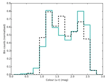
Figure 4.We show a normalised histogram of the colours in the SAMI Galaxy Survey sample (blue) and the sample used in this work (black, dashed). The data used were taken from the GAMA Data Release 2 catalogue SpecLineSFR (Hopkins et al. 2013).
Bi
n
co
un
ts
(n
or
m
al
is
ed
)
Figure 5.We show a normalised histogram of the specific SFR in the SAMI Galaxy Survey sample (blue) and the sample used in this work (black, dashed). The data used were taken from the GAMA Data Release 2 catalogues SpecLineSFR (Hill et al. 2011) and StellarMasses (Taylor et al. 2011).
3 USING KINEMETRY TO QUANTIFY
KINEMATIC ASYMMETRY
3.1 The kinemetry algorithm
Kinemetry is an extension of photometry to the higher order moments of the line of sight velocity distribution (LOSVD)2. It was developed as a means to quantify asymmetries in stel-lar velocity (and velocity dispersion) maps. These anomalies may be caused by internal disturbances or by external fac-tors, namely interactions (Krajnovi´c et al. 2006).
2 The kinemetry code is written in IDL, and can be found at
http://davor.krajnovic.org/idl/(Krajnovi´c et al. 2006).
The method works by modelling kinematic maps as a sequence of concentric ellipses, with parameters defined by the galaxy centre, kinematic position angle (PA) and ellip-ticity. It is possible to fit the latter two parameters within kinemetry, or to determine them by other means and exclude them from the fitting procedure. For each ellipse, the kine-matic moment is extracted and decomposed into the Fourier series:
K(a, ψ) =A0(a) + N X
n=1
(An(a)sin(nψ) +Bn(a)cos(nψ)),(1)
whereψis the azimuthal angle in the galaxy plane, andais the ellipse semi-major axis length. Points along the ellipse perimeter are sampled uniformly inψ, making them equidis-tant in circular projection. The series can be expressed more compactly, as (Krajnovi´c et al. 2006):
K(a, ψ) =A0(a) + N X
n=1
kn(a)cos[n(ψ−φn(a))], (2)
with the amplitude and phase coefficients (kn, φn) defined
as:
kn= p
A2
n+Bn2 (3)
and
φn=arctan An
Bn
. (4)
The moment maps for both velocity and velocity disper-sion can thus be described by the geometry of the ellipses and power in the coefficientskn of the Fourier terms as a
function ofa(Krajnovi´c et al. 2006).
The velocity field of a completely normal, rotating disk would be entirely contained in thecos(ψ) term of Equation 2, with zero power in the higher order modes, since the ve-locity peaks at the galaxy major axis and goes to zero along the minor axis. As a result, the power in theB1 term
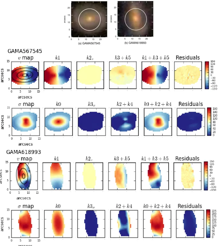
rep-resents circular motion, with deviations carried in the other coefficients. Fig.6shows results of kinemetric fitting to the Hα velocity maps of a normal and an asymmetric galaxy in our sample. For the normal galaxy (top), GAMA567545, all the power is in the first order moment (k1), whereas the
asymmetric galaxy (bottom), GAMA628993, has significant power in the higher order modes (k3+k5).
Analogously to the velocity field, a map of the velocity dispersion field of a perfectly normal rotating disk would have all power in theA0term (i.e. radial dispersion gradient)
(Krajnovi´c et al. 2006). The velocity dispersion field is an
even moment of the LOSVD, and therefore its kinemetric analysis reduces to traditional surface photometry.
Kinemetry contains routines to fit the PA and ellip-ticity of the input kinematic fields. These inbuilt routines were used on the high S/N data fields from the ATLAS3D survey. Similarly to the SINS survey (Shapiro et al. 2008), we found that the lower S/N of the SAMI Galaxy Survey fields, compared to ATLAS3D data, led to unstable fits to these parameters. We used the PA and ellipticity from the single Sersic fits to the SDSSr-band images in the GAMA Survey DR2 catalogue SersicCat (Kelvin et al. 2012). This is a reasonable step for disturbance measures because, for kinematically normal rotating galaxies, the photometric and kinematic PA should agree. This is not the case for galaxies
0 5 10 15 20 (a) GAMA567545 20
15
10
5
0
ar
cse
cs
0 5 10 15 20
(b) GAMA618993
20
15
10
5
0
ar
cse
cs
with misaligned kinematic and photometric PAs. However, we find that galaxies with misaligned PAs are generally clas-sified as visually asymmetric (see Section3.3).
3.2 Using kinemetry to measure kinematic asymmetry
We perform kinemetry on the Hαvelocity and velocity dis-persion maps for all 360 galaxies in our sample. Following work on the SINS survey (Shapiro et al. 2008), we calcu-late radial kinematic asymmetry values for the velocity and velocity dispersion fields of each galaxy, respectively:
vasym=
k3,v+k5,v
2k1,v
σasym=
k2,σ+k4,σ
2k1,v
, (5)
We have slightly modified the method of Shapiro et al.
(2008) that fit all moments (odd and even) when calculating both velocity and velocity dispersion asymmetry:
vasym,SIN S=
k2,v+k3,v+k4,v+k5,v
4k1,v
(6)
σasym,SIN S=
k1,σ+k2,σ+k3,σ+k4,σ+k5,σ
5k1,v
, (7)
They did this because they were specifically looking for the signatures of major mergers, which produce extremely dis-turbed velocity fields, with power in all higher order mo-ments (Shapiro et al. 2008). Due to the comparatively small amplitude of the kinematic asymmetries in our sample, we found the asymmetry contributions of even moments to velocity asymmetry to be negligible (see velocity fields of GAMA618993 in Fig. 6for an example), and similarly for the contributions of odd moments to the velocity dispersion asymmetry. Accordingly, we used only odd moments for the velocity fields and the even moments for the velocity dis-persion, as was done for ATLAS3D data (Krajnovi´c et al.
2011).
Krajnovi´c et al. (2006) note that, when studying the
velocity dispersion of the stellar component of the galaxy, it is appropriate to normalise over the zeroth moment of the velocity dispersion. We, however, followShapiro et al.(2008) in normalising both quantities over the velocity (k1), rather
than the velocity dispersion, because the velocity dispersion of the gas component of a galaxy is extremely sensitive to shocks and other features. This makes normalising to the rotation curve (the first moment of the velocity) a more reliable choice, as it is not as sensitive to these features, but is sensitive to the potential.
To determine the centre of the kinematic maps used in this analysis, we fit a 2-dimensional Gaussian to the SAMI Galaxy Survey r-band continuum flux maps and took the centroid of the location of the 25 brightest spaxels in a 6x6 pixel area around the centre of the fitted Gaussian. We did not use the the Hα emission maps because they contain clumps of star formation and other features, which make determining the centre from these maps potentially unreli-able.
In order to accommodate the effects of covariance out-lined in Section2.2, we altered the kinemetry fitting routine, such that the spacing between ellipses was constrained to be≥2.5 arcsecs. The effective covariance diameter is∼2.5 arcsecs, so this ensures that data points used by adjacent el-lipses are independent of each other. The 1-σerrors onvasym
2 3 4 arcsecs5 6 7 8
0.00 0.05 0.10 0.15 0.20 0.25
v
asym2 3 4 arcsecs5 6 7 8
0.00 0.05 0.10 0.15 0.20 0.25 0.30 0.35 0.40 0.45
σ
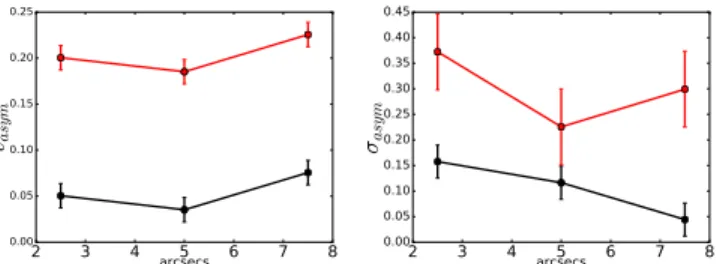
asymFigure 7.We show the values ofvasym(left) andσasym(right), with 1-σ errors, at the positions of the semi-major radii of the fitted ellipses for an asymmetric (red, GAMA618993) and non-asymmetric (black, GAMA567545) galaxy. It can clearly be seen that the velocity and velocity dispersion asymmetry values for the asymmetric galaxy are significantly higher than those of the normal galaxy. These are the same two galaxies shown in Fig.6.
andσasymwere then bootstrapped to produce the errors on
vasymandσasym. The bootstrapping involved 100 iterations
of adding random noise to the velocity and velocity disper-sion fields, and then recalculating the median ofvasym and
σasym. The final values for the errors on vasym and σasym
are taken from the scatter in the results of the iterations. Be-cause of the enforced separation between ellipses, we only fit across three kinemetric ellipses for each galaxy (see Fig.6). This does entail the possibility of losing detail, as small kine-matic asymmetries may be lost ‘between’ successive ellipses. It is also possible that small features identified in the mor-phological classification in Section 3.3may not be detected using this method. However, due to covariance, a more finely sampled kinematic fit would not increase the accuracy of our results. The qualitative nature of the visual classifica-tion means that we cannot quantitatively define a lower limit for the size of features that caused a galaxy to be classified as ‘definitely asymmetric’. However, the process focussed on large-scale features, such as tidal tails.
In Fig. 7, vasym and σasym are plotted at the
semi-major radii of each of the fitted ellipses for a visually nor-mal and an asymmetric galaxy (the same galaxies as shown in Fig.6). We see that the visually asymmetric galaxy (in red) has consistently higher kinematic asymmetry than the visually normal galaxy.
We take the median of vasym and σasym over all
el-lipses (relative to the centre of the continuum emission), so that each galaxy’s total kinemetric asymmetry can be ex-pressed as the combination ofvasymandσasym. Fig.8shows
σasymagainstvasymfor the whole sample and for three mass
bins. A discussion of the relationship between stellar mass and vasym can be found in Section6. As in Shapiro et al.
(2008), it will be useful to define a cutoff on this plane, above which galaxies may be considered kinematically asymmet-ric. Given that bothσasym against vasym form continuous
distributions, it is not immediately obvious, based purely on kinematics, where to draw such a cutoff. Accordingly, we use visual classification to provide a guide.
3.3 Visually classifying asymmetric galaxies
The 360 galaxies in our sample were morphologically classi-fied visually, by members of the team, usinggricomposite images from the SDSS DR10 catalogue (Ahn et al. 2014).
Figure 8.These plots summarise the results of kinemetry for the 360 galaxies in our sample (top) and three stellar mass bins (bottom row). The median kinemetric asymmetries for both velocity and velocity dispersion across fitted ellipse radii are normalised over the rotational velocity and plotted against each other. The sample was visually classified morphologically (using the SDSS DR10 images), with visually asymmetric galaxies shown here in red, and ‘possibly asymmetric’ galaxies in yellow. We show thevasymcutoff for kinematic asymmetry derived in the text (blue, dashed line). The two example galaxies from Fig. 6, GAMA567545 (the normal galaxy) and GAMA618993 (the asymmetric galaxy) are indicated by the green arrows, for reference.
The SDSS DR10 catalogue has sufficient depth and spa-tial resolution to show the large-scale features relevant to our work. The median seeing, defined as the FWHM of the point spread function, in the SDSS sample is 1.43” in ther -band. This is much smaller than the median effective radius of galaxies in the SAMI Galaxy Survey sample, 4.4” (Bryant
et al. 2015). The features that define morphological
asym-metry for this paper (e.g. double cores and large tidal tails) are larger than the seeing in the SDSS DR10 images. The SDSS DR10 images have been previously successfully used to identify large-scale features such as mergers in Galaxy Zoo (Darg et al. 2010;Casteels et al. 2013).
Of course, visual classification is a qualitative approach, and vulnerable to bias or error. We compensated for this by
having multiple people classify each galaxy, with an average of 5 individuals classifying each galaxy.
The categories for classification were (with quoted in-structions for classification into each group and number of galaxies sorted into each category):
• normal: “No evidence of interaction. These galaxies are almost completely smooth and symmetrical.” 246 galaxies
• definitely visually asymmetric: “These galaxies do not have to be major merger remnants, but are nevertheless clearly distinguishable from normal/slightly/possibly asym-metric galaxies. They might have evidence of a double core, extremely distorted spiral arms, or long tidal tails, indicat-ing a major interaction.” 81 galaxies
indicat-ing some interaction with a passindicat-ing galaxy, or might show evidence of a very minor merger.” 19 galaxies
• uncertain: “Galaxies that are small or unclear enough that a reliable classification is impossible.” 15 galaxies
Fig.9shows examples of galaxies in the normal, definitely vi-sually asymmetric and uncertain categories. The features in-cluded in the ‘definitely visually asymmetric’ category were: tidal tails, warps, and evidence of double cores or in-progress mergers. Importantly, we were not simply identifying major mergers, but rather a range of visual asymmetries. If there was at least 66% agreement that a galaxy was ‘definitely vi-sually asymmetric’, it was placed in the vivi-sually asymmetric sample used throughout this work. Individual classification results are given in the appendix to this paper.
We note the similarity of our method to that used by the IMAGES survey (Yang et al. 2008) to classify kinematic maps. However, unlike the IMAGES survey work, we used a qualitative approach to identify visual asymmetry and a quantitative standard for kinematic asymmetry.
We chose to be conservative in excluding galaxies that were only possibly visually asymmetric from the list of visu-ally asymmetric galaxies. This was because we did not want to err on the side of misclassifying normal galaxies as visu-ally asymmetric. For our purposes, it was better to have a cleaner sample of visually asymmetric galaxies, even at the potential cost of losing a small fraction. Similarly, galaxies with apparent near companions, but no visual evidence of asymmetry, were classified as normal.
We find no difference in the errors on the SDSS pho-tometric PAs for galaxies classified as visually asymmetric and normal. Galaxies with offset kinematic and photometric PAs were generally visually classified as asymmetric. The relationship between offset between kinematic and photo-metric PAs and kinematic asymmetry will be the subject of future work by the SAMI Galaxy Survey team (Bryant et al., in prep, Bloom et al., in prep). An offset between the kinematic and photometric PA would likely qualify a galaxy as ‘asymmetric’ for the purposes of this work.
4 DISTINGUISHING BETWEEN
KINEMATICALLY NORMAL AND
ASYMMETRIC GALAXIES IN THE SAMI GALAXY SURVEY
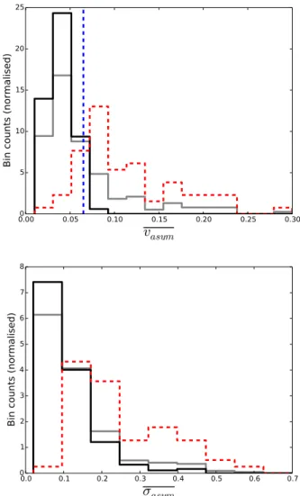
Fig10shows histograms of the distributions of median veloc-ity and velocveloc-ity dispersion asymmetries, vasym andσasym.
The complete sample is shown in grey. The distribution in both cases is smooth, and peaked at low values, with a tail. It is not immediately obvious where to place a cutoff for galaxies to be classified as kinematically asymmetric or nor-mal.
Fig10also shows galaxies visually identified as metric in red, and normal galaxies in black. Visually asym-metric galaxies tend to have highervasymandσasym, which
provides a reasonable basis for the cutoff.
The good agreement between the visual classification and measured kinematic asymmetry suggests that, if there is kinematic disturbance, the image will almost always show a signature of that disturbance. While kinematics provide a more physical measure of disturbance, the images show
0 5 10 15 20
(a) GAMA567545: ‘normal’ 0
5 10 15 20
arcsecs
0 5 10 15 20
(b) GAMA375531: ‘definitely asymmetric’ 0
5 10 15 20
arcsecs
0 5 10 15 20
(c) GAMA383259: ‘possibly asymmetric’ 0
5 10 15 20
arcsecs
Figure 9.From top left we give: examples of ‘normal’, ‘definitely visually asymmetric’, and ‘possibly visually asymmetric’ galaxies from the morphological classification. The SAMI instrument field of view is shown as a white circle. Images are from the SDSS DR10 catalogue used to classify the galaxies.
the effects of that disturbance. Galaxies ‘incorrectly’ visu-ally classified cannot be quantitatively distinguished, due the qualitative nature of the visual classification.
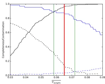
Fig.11shows the fractional completeness and contam-ination from 0 to 1.0 of the samples of visually asymmet-ric and normal galaxies across a range of values on either side of the crossover points of the visual classification his-tograms in Fig.10, forvasym. Ideally, we would like to
max-imise completeness (which we define as fraction of galaxies with the same kinematic classifications as visual) and min-imise contamination (defined as fraction in each kinematic bin with opposite visual classifications) for both visually nor-mal and asymmetric galaxies. The distance between the in-tersection points of the curves for visually normal and asym-metric galaxies indicates how viable it is to choose a single kinematic cutoff point for that purpose. We found that the distance between intersection points was much greater for
σasymthan forvasym(0.032 against 0.013). This means that
it is significantly harder to choose a cutoff based onσasym
that will give both high completeness and low contamina-tion for both normal and asymmetric galaxy populacontamina-tions. This is the case whether we try a cut based onσasym or a
combination withvasym.
Accordingly, we cut by median velocity asymmetry,
vasym. The intersection points of the curves representing
contamination and completeness are 0.071 and 0.058, respec-tively. We thus choose the midpoint of these values, giving a cutoff value ofvasym >0.065 for a galaxy to be
consid-ered asymmetric (shown in blue in Fig 10). This yields a contamination of 3% and completeness of 90% for visually asymmetric galaxies, and contamination of 10% and com-pleteness of 95% for visually normal galaxies. Of course, the
by-eye classification we take as our guide is imperfect and qualitative, so there is some uncertainty in these measures. Nevertheless, the degree to which it is possible to map the visual classification onto the kinemetric one does point to an underlying physical similarity between the features selected for by each.
The red points in Fig.8are galaxies classified as visually asymmetric, and the black points are visually normal galax-ies. The larger scatter between the visually asymmetric and normal galaxies in σasym shows again that more visually
asymmetric galaxies would be misclassified as asymmetric by applying a cutoff in bothvasymandσasym. We note that
the SINS survey team also used the mean of the higher order mode values, whereas we took the median. We found that taking the mean increased the contamination between the distributions of visually asymmetric and normal galaxies. A similar analysis to that performed above yielded a crossover contamination of 8% for visually asymmetric galaxies.
We also show galaxies classified as visually ‘possibly vi-sually asymmetric’ in yellow in Fig. 8. We note that these galaxies are almost all (90%) in the lower section, or ‘nor-mal area’ of the plot, with only two galaxies falling above our vasym >0.065 line. This supports our decision to
ex-clude them from the sample of visually asymmetry galaxies. Galaxies classified as visually normal but kinematically asymmetric are clustered around the boundary value of
vasym∼0.065. The qualitative visual classification does not
allow us to further distinguish these galaxies. The advan-tage of kinemetry is that it removes this qualitative compo-nent. Of the galaxies classified as morphologically perturbed but kinematically normal, some have images which appear to include foreground objects, which may contribute to the ‘misclassification’.
We note that galaxies in the sample have different ef-fective radii, so are covered to different extents by the SAMI instrument field of view. We do not, however, find that cov-erage influences the outcome of fits by kinemetry, so we dis-regard this as a possible bias in our results.
Using our kinemetry results, and cutting the sample at
vasym>0.065, we calculate a kinematic asymmetric fraction
of 23%±7%. This is comparable to the complex kinematics fraction of 26%±7 calculated by the IMAGES survey (Yang
et al. 2008) for galaxies withz∼1, using a visual
classifica-tion method similar to ours described in Secclassifica-tion 3.3.
4.1 Comparison of the kinemetry technique with quantitative morphology
Given that major mergers are known to cause kine-matic asymmetry (Shapiro et al. 2008), we determine whether quantitatively morphologically asymmetric galax-ies are kinematically asymmetric, and whether kinemat-ically asymmetric galaxies are quantitatively morphologi-cally distinct from kinematimorphologi-cally normal galaxies. Quanti-tative morphology techniques, such as the Gini (Gini 1912)
andM20(Lotz et al. 2004) coefficients, and the
Concentra-tion/Asymmetry/Smoothness (CAS) categorisation method
(Conselice 2003) have been used in previous studies to
iden-tify major mergers, as has kinemetry (Shapiro et al. 2008), providing a useful basis for comparison.Simons et al.(2015) compare σ
V and quantitative morphology, concluding that
kinematically disturbed galaxies, falling off the Tully-Fisher
0.00 0.05 0.10 0.15 0.20 0.25 0.30
v
asym
0 5 10 15 20 25
Bin counts (normalised)
0.0 0.1 0.2 0.3 0.4 0.5 0.6 0.7
σ
asym
0 1 2 3 4 5 6 7 8
Bin counts (normalised)
Figure 10.We show normalised histograms ofvasym(top panel) andσasym(bottom panel) for the whole sample (grey), visually classified normal (black) and asymmetric (red, dashed) galaxies. The cutoff value,vasym= 0.065, is shown in blue.
line, also tend to be asymmetric by the standards of quan-titative morphology.
To perform this analysis, we use ther-band SDSS DR10 images (Ahn et al. 2014). We follow methods inLotz et al.
(2004) andConselice(2003). To determine the centre of the images used in this analysis, we replicate the method de-scribed in Section3on ther-band SDSS DR10 images for each galaxy.
In this work, errors onG,M20and the CAS Asymmetry
coefficient are found by bootstrapping the calculations of the coefficient for each galaxy, adding random noise to the data and calculating the uncertainties from the distribution of these iterations.
4.1.1 The Gini coefficient
The Gini coefficient,G, was developed by economists (Gini 1912) as a descriptor of the distribution of resources amongst a population. G = 1 indicates that the entire wealth of a population is concentrated with one individual, whereas
0.03 0.04 0.05 0.06 0.07 0.08 0.09
v
asym0.0 0.2 0.4 0.6 0.8 1.0
Completeness/Contamination
Figure 11.These curves show contamination (dashed) and com-pleteness solid for visually asymmetric (blue) and visually normal (black) galaxies, at a range of values ofvasym. We choose our cut-off point (shown in red) as the midpoint between the points of intersection of the curves for contamination (number of visually normal galaxies classified as kinematically asymmetric and vice versa) and completeness (number of visually asymmetric galax-ies classified as kinematically asymmetric, similarly for visually normal galaxies) (shown in green). The points of intersection for contamination and completeness are 0.071 and 0.058, respectively, so we choose a cutoff value ofvasym=0.065. See Section4for a complete explanation.
astronomical context byAbraham et al.(2003). Applied to galaxy flux,Gbecomes a measure of concentration of light, similar toCin the CAS system (see Section4.1.3). In
high-G galaxies, the light is locally concentrated (for instance, there could be a highly dominant bulge). A low-G galaxy would have a smooth, uniform light distribution, without a significant bulge. Alternatively, it could be composed of many small clumps, including regions of star formation that would ‘balance out’ a central bulge.
Gis mathematically defined as (Glasser 1962):
G= 1
Xn(n−1)
n X
i
(2i−n−1)Xi, (8)
where X is (in this case) the mean of the galaxy flux inn
total pixels, withXibeing the flux in theith pixel.
Previous work has used G in combination with M20
(Lotz et al. (2004), see Section4.1.2) and CAS (Conselice
(2003), see Section4.1.3) to identify major mergers.
4.1.2 TheM20coefficient
TheM20 coefficient is similar toG, in that it measures the
concentration of the spatial distribution of light within a galaxy, but can be used to distinguish galaxies with differ-ent Hubble types (Lotz et al. 2004). The total second-order moment of galaxy flux,Mtot, is defined as the fluxfiin each
pixel, multiplied by the squared distance between pixeliand the centre of the galaxy (xc, yc), summed over all galaxy
pix-els:
Mtot= n X
i
Mi= n X
i
fi[(xi−xc)2+ (yi−yc)2]. (9)
M20is then defined as the normalised second-order
mo-ment of the brightest 20% of the galaxy’s flux. The galaxy pixels are rank-ordered by flux, and then Mi (the
second-order moment of light for each pixeli) is summed over the brightest pixels until the sum of the brightest pixels is equal to 20% of the total flux:
M20=log10 P
iMi
Mtot
(10)
forP
ifi<0.2ftot, whereftotis the total flux, Pn
i fi.
4.1.3 CAS Asymmetry
The CAS (Concentration, Asymmetry, Smoothness) system was developed as a means to distinguish galaxies in differ-ent stages of evolution, based on where they fall within a volume derived from the CAS structural parameters (
Con-selice 2003). TheC andA parameters were first developed
byAbraham et al. (1996). We will discuss only the
appli-cation of Asymmetry, henceforth A, as C and S are not intended to describe asymmetries.
To findA, a galaxy image is rotated 180◦ around its central point and the result is subtracted from the original image.Ais then computed as the sum of the absolute values of the residuals, normalised over the sum of the flux in the original image.A is clearly sensitive to any feature that is not rotationally symmetric. These may include spiral arms, areas of intense star formation, and merger signatures (
Con-selice 2003).
It is important to note thatAwas specifically developed to identify the middle stage of major mergers, in which case the visual asymmetric features resulting from the merger would far outweigh those from ordinary morphology, such as spiral arms. However, in the case of more minor asymme-tries, other morphological features may dominate. For ex-ample, a relatively small and dim tidal tail would be over-shadowed by the presence of bright spiral arms.
4.1.4 Comparison of classifications using kinematics and quantitative morphology
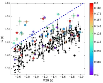
Following previous work (Lotz et al. 2004), Fig.12 shows
M20 against G for the galaxies in our sample. The
kine-matically asymmetric galaxies (coloured) are those with
vasym>0.065.Lotz et al.(2004) drew a line on the plane to
distinguish ULIRGS from ‘normal’ galaxies, shown in Fig.12
in dashed blue. Whilst all of the galaxies above the line in our sample are kinematically asymmetric, there are also many kinematically asymmetric galaxies which would not be identified using this method. Quantitatively, 79%±3% of kinemetrically asymmetric galaxies would be classified as normal by this method. Further, many of the most kine-matically asymmetric galaxies, indicated by the colour bar, fall below the line. This is becauseGandM20measure the
spread of light. A galaxy with multiple, bright clumps has a different light distribution profile from a normal galaxy (with one bright, central bulge), but a galaxy with a strong kinematic twist may not, as the ratio of light in the bulge
2.0 1.8 1.6 1.4 1.2 1.0 0.8 0.6
M20 (r)
0.35 0.40 0.45 0.50 0.55 0.60
G (r)
0.07 0.085 0.099 0.113 0.128 0.142 0.157 0.171 0.186 0.2
Figure 12.We showM20againstG, with kinemetric classifica-tions (normal galaxies in black, kinematically asymmetric galax-ies in colour). We see that, even though the majority of galaxgalax-ies falling above the line defined inLotz et al.(2004) are kinemat-ically asymmetric, there are many that would not be identified using this system. The colourbar shows thevasymvalues on a log scale for the kinematically asymmetric points. We see that many of the most kinematically asymmetric points fall below the line.
and body of the galaxy may be the same, regardless of the twist.
In Fig. 13, following Conselice et al. (2008), we show
Gagainst A. As in Fig. 12, coloured points are those with
vasym>0.065. We once again see only a weak relationship
between kinematic asymmetry and placement on the plane. Galaxies withA >0.4 are mostly kinematically asymmetric, but below this threshold there is no significant relation. In-deed, 59%±4% of kinematically asymmetric galaxies in our sample lie below A= 0.4. As in Fig.12, some of the most kinematically asymmetric galaxies are not classified as mor-phologically disturbed using this method. This is because the relationship between A and photometric (also, by ex-tension, kinematic) asymmetry becomes significantly weaker belowA= 0.4 (Conselice 2003;Conselice et al. 2008). Whilst galaxies withA >0.4 are very likely to be disturbed, below this threshold normal morphological features (particularly spiral arms) dominate, so true asymmetries are lost. Given that most of our kinematically asymmetric galaxies fall be-low this threshold, our result is not unexpected.
We conclude that almost all quantitatively morpholog-ically asymmetric galaxies are kinematmorpholog-ically asymmetric. Further, kinematics can identify asymmetry in galaxies that appear normal when using these quantitative morphology methods.
5 COMPARISON OF OUR RESULTS WITH HIGH REDSHIFT STUDIES
Although our method is based on that used by the SINS Survey team, there are some differences. For example, they used the mean of radially calculated kinematic asymmetry values, whereas we used the median, and they included the even modes of the velocity fields and odd modes of velocity
0.0 0.1 0.2 0.3 0.4 0.5 0.6 0.7 0.8
A (r)
0.35 0.40 0.45 0.50 0.55
G (r)
0.07 0.085 0.099 0.113 0.128 0.142 0.157 0.171 0.186 0.2
Figure 13.We show theA−Gplane for kinematically normal (black) and kinematically asymmetric (coloured) galaxies. Errors are 1-σerrors on both axes. As anticipated, only a weak relation emerges between asymmetry and plane location. The blue line indicatesA sim0.4, below which the relationship betweenAand asymmetry becomes significantly weaker.
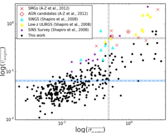
dispersion fields in the calculation of velocity and velocity dispersion asymmetry. In order to more directly compare our results with the SINS Survey results, we recalculated our kinematic asymmetry values, applying their method. Fig14
shows our results (black points), along with a sample of those from the SINS Survey, including artificially redshifted local spiral galaxies from the SINGS Survey (turquoise triangles), artificially redshifted local ULIRGS (yellow triangles) and galaxies observed by the SINS Survey team at high red-shift (purple points) (Shapiro et al. 2008). We also show a sample of high redshift (2.0 < z < 2.7) sub-millimetre galaxies (SMGs) from Alaghband-Zadeh et al. (2012) (red crosses). Of the SMGs, those which are AGN candidates are also noted (red diamonds superimposed on the red crosses). We see that the spread of our values does not change signif-icantly, despite the recalculation.
Applying their version of kinemetry to the SINS Sur-vey sample led to an estimated major merger fraction of
∼25% (Shapiro et al. 2008). Due to the high redshift of their sample (z ∼2), which led to correspondingly low HαS/N in their data, even their normally-classified galaxies have higher kinematic asymmetry values than the majority of the galaxies in our sample (see Fig14).Gon¸calves et al.(2010) have argued that, in fact, degrading the resolution of data (as a proxy for higher redshift) leads todecreasedkinematic asymmetry values, rather than the increased values found by the SINS Survey. However, it is not clear how a corre-sponding increase in noise for high-redshift data will affect the results. This is a still open question and, accordingly, our result of a kinematic asymmetric fraction of 23%±7% should not be directly compared with the result inShapiro
et al.(2008). The SINS Survey also required their galaxies to
have continuum S/N≥3 that may have biased their sample towards galaxies with high SFR, influencing the distribution of kinematic asymmetries.
Figure 14.This figure shows the mean velocity and velocity dis-persion asymmetries for galaxies in our sample and those from several other works using kinemetry (as in legend). Error bars have been removed for clarity. The grey lines indicate the kine-matic asymmetry cutoffs from the SINS Survey work (Shapiro et al. 2008), and the blue line is the cutoff we developed for use on our data.
and artificially redshifted) fall entirely above our cutoff for kinematic asymmetry, with the exception of two redshifted SINGS spiral galaxy. Given the results from the SINS Sur-vey, that showed how decreased S/N (either artificially or from increased redshift) can increase kinemetric coefficients, this is not surprising. Nevertheless, the higher kinemetric co-efficients may also be reflective of intrinsic kinematic asym-metry.
If we were to naively apply the cutoff from the SINS Sur-vey work (mean velocity and velocity dispersion asymmetry = 0.5), we would have a major merger rate of 1±4%. There have been a number of other local merger rates, including those calculated using simply close pairs (e.g. De Propris
et al. 2014), quantitative morphology (e.g.Lotz et al. 2008,
2011) and a combination of the two methods (Casteels et al. 2014). These local major merger rates range from∼1-4%, and so are broadly consistent with the value from this work combined with the SINS Survey cutoff. However, given the difference in redshift between the SINS Survey and SAMI Galaxy Survey, this should not be interpreted as necessarily signifying scientific agreement. Atz∼1,Stott et al.(2014) use kinemetry (approximately following the Shapiro et al. 2008) method, using a cutoff ofKtot>0.5) to derive a
ma-jor merger rate of 10%.
We further note that, of the SAMI Galaxy Survey sam-ple galaxies that fall above the SINS Survey cutoff, 66% fall above the major merger lines in Fig.12and Fig.13.
6 THE RELATIONSHIP BETWEEN
KINEMATIC ASYMMETRY, COLOUR AND STELLAR MASS
Colour is directly linked to star formation history. We in-vestigate whether processes causing kinematic asymmetry influence star formation history, as revealed by a change in
7.5 8.0 8.5 9.0 9.5 10.0 10.5 11.0 11.5
log(M∗)
0.5 1.0 1.5 2.0 2.5
Colour (u-r) (mag)
Figure 15.This plot gives colour and stellar mass for the sample used in this work of kinematically identified normal (black) and kinematically asymmetric galaxies (green). The dark blue line separates the blue cloud and red sequence, and is taken from
Schawinski et al. (2014). The data used were taken from the GAMA Data Release 2 catalogues StellarMasses and ApMatched-Photom (Hill et al. 2011;Taylor et al. 2011).
colour. Several studies have established links between colour and kinematic abnormality, e.g.Conselice et al.(2000);
Kan-nappan et al.(2002);Neichel et al.(2008), finding that
asym-metric galaxies are bluer than their normal counterparts. We here determine the position of our sample of kinematically asymmetric galaxies on the colour-stellar mass plane. Fig.15
shows theu−rrest frame colour-stellar mass distribution for normal (black) and kinematically asymmetric (green) galax-ies. We used a cut fromSchawinski et al.(2014) (dark blue in Fig.15) to separate the blue cloud and red sequence. We see that 75±10% of kinematically asymmetric galaxies fall in the blue cloud, and only 25±11% fall on the red sequence. For comparison, 65±7% of normal galaxies are in the blue cloud, and 34±8% of normal galaxies are in the red sequence. Fig. 16 shows an inverse relationship between stellar mass and kinematic asymmetry, and a Spearman rank cor-relation test forvasym and stellar mass givesρ=−0.30,
p-value= 8.40×10⁻⁹. We further show the fraction of
kinemat-ically asymmetric galaxies in bins of stellar mass that also dramatically declines with increasing stellar mass. Given that colour and stellar mass are strongly correlated, the ap-parent tendency of kinematically asymmetric galaxies to be bluer, compared to their normal counterparts, is not surpris-ing.
To test whethervasym and colour are related
indepen-dently of mass, we performed a series of partial Pearson correlation tests betweenvasym and colour (accounting for
the correlation of colour with stellar mass) on the individual branches and the whole sample. The results of the correla-tion test between colour and vasym for the red and blue
branches were ρ =0.054, p-value= 0.57 and ρ =0.096, p-value= 0.13, respectively. For the whole sample the result was ρ =0.11, p-value= 0.028. This indicates that there is at best marginal correlation between colour and kinematic
0.0 0.1 0.2 0.3
v
asym7.5 8.0 8.5 9.0 9.5 10.0 10.5 11.0 11.5
log
(
M
∗)
0.0 0.1 0.2 0.3 0.4 0.5
Fraction of galaxies above cutoff
Figure 16.vasymis plotted against against stellar mass for the galaxies in our sample. The orange line shows our kinematic metry cutoff, such that all galaxies above it are considered asym-metric. The bottom panel shows the fraction of galaxies, in bins of stellar mass (shown as horizontal error bars), above the asym-metry cutoff. This fraction decreases as a function of stellar mass.
asymmetry, either in the separate branches or the full sam-ple.
The small positive correlation betweenvasymand colour
over the full sample is explained by a slight deficit of high mass, blue branch kinematically asymmetric galaxies in Fig.
15. Examining the proportion of kinematically asymmet-ric galaxies in each branch above log(M∗) > 10.0, 15 of 86 (17±3%) of red galaxies are kinematically asymmetric, compared to 7 of 66 (10±3%) of blue galaxies. Although the difference is marginally significant, a possible physical explanation for this comparative deficit of high-mass, blue branch kinematically asymmetric galaxies may be related to the lower gas fraction in red galaxies. Incoming gas from an interaction is likely to settle to rotate with the main galaxy mass in a high-gas fraction (blue) galaxy. However, in a low-gas fraction, red galaxy, it may be easier to preserve any difference in angle of rotation between newly accreted gas and the main disk. Given that, for kinemetry, we fit the PA of the disk fromr-band photometry that traces the stellar component, any offset in the PA of the gas would register in the higher order moments [Bryant et al., 2016 (in prep)].
Fig.17shows a histogram of the distance of each galaxy from the red/blue cutoff in Fig. 15, in terms of colour, as well as the medians of the distributions. A negative dis-tance indicates that the galaxy is in the blue branch, whereas red galaxies have positive distances. A negative shift in the median distance would indicate that kinematically asym-metric galaxies are bluer than normal galaxies, independent of the negative correlation between mass and vasym. The
medians are -0.14±0.014 (normal galaxies) and -0.18±0.027 (kinematically asymmetric galaxies). There is an offset of 0.03±0.03, which is not significant. From this result, we conclude that the dominant relationship is between vasym
and stellar mass.
1.0 0.8 0.6 0.4 0.2 0.0 0.2 0.4 0.6 0.8
Distance from Red/Blue Cutoff 0.0
0.5 1.0 1.5 2.0 2.5
Figure 17. We show a normalised histogram of distance (in colour space) from red/blue cutoff for kinematically asymmet-ric (red) and normal (black, dashed) galaxies. The median offset for each distribution is shown by the vertical lines. There is no significant offset between the kinematically asymmetric and nor-mal medians, indicating that, independent of mass, there is no relationship between colour andvasym.
6.1 Explaining the inverse correlation between stellar mass andvasym
There are several possible reasons for the strong observed relationship between mass and kinematic asymmetry. We rule out that the increasedvasymis a result of poorer S/N in
the low-mass objects, as there is no significant trend between the HαS/N and galaxy mass. Further, there is no statistical relationship between the number of effective radii covered in the analysis and kinematic asymmetry, which excludes any boost invasymin low-mass galaxies purely due to their size.
This is because the low-mass galaxies in the SAMI Galaxy Survey sample are at lower redshift and have proportionately more Hαgas (Allen et al. 2015).
The Tully-Fisher relation (Tully & Fisher 1977) links the rotational velocity of galaxies to their absolute magni-tude, which is, in turn, proportional to stellar mass. The dwarf galaxies in our sample have lower rotational velocities than high-mass galaxies. Given that, in this work, higher or-der kinemetry terms are normalised relative to the first oror-der velocity field, it is plausible that kinematic asymmetries of the same intrinsic amplitude would yield greater kinemetric signatures in low-mass galaxies, as low mass galaxies have disproportionately low velocities. Low mass galaxies have also previously been found to have complex kinematics by a variety of metrics [e.g.van Zee et al.(1998);Cannon et al.
(2004);Lelli et al.(2014)]. Further, alternative measures of
kinematic asymmetry, such as that in the rotation curve
(Barton et al. 2001;Garrido et al. 2005), have found dwarf
galaxies to have both high kinematic asymmetry and low ro-tational support . It has additionally been long established that low-mass galaxies have irregular morphologies (Roberts
& Haynes 1994;Mahajan et al. 2015; Simons et al. 2015),
that may be linked to their irregular kinematics.
Escala & Larson(2008) link the stochastic formation
the mass of gaseous instabilities is inversely proportional to angular rotational velocity:
Mclmax=
π4G2Σ3 gas
4Ω4 , (11)
whereMclmaxis the maximum mass of unstable regions, Σ is
the gas surface density and Ω is the angular rotation speed,
Vc(R)
R , of the disk. Given that, in order to meet the condition
for rotational support inside a given radiusR,
Ω2= πGΣgas
νR , (12)
where ν =Mgas/Mtot, the maximum instability mass can
be expressed as a function of gas fraction:
Mclmax=
π2ν2R2Σgas
4 . (13)
Given their typically high gas fractions (Geha et al.
2006;Huang et al. 2012), i.e. highν, low-mass galaxies are
likely to have comparatively large maximal sizes of these instabilities. Assuming that large instabilities leave kine-matic signatures corresponding to increased kinemetric co-efficients, this effect may contribute to the trend observed here. This theory is supported by work such asAmor´ın et al.
(2012), in which complex Hαkinematics in dwarf galaxies are linked to the presence of multiple star-forming clumps. Further,Green et al.(2013) find that, for star-forming galax-ies, high gas fraction (inferred from SFR density) is linked to high σm
V , whereσmis the mean velocity dispersion, andV is
the circular velocity. This measure can be used as a proxy for turbulent support, relative to rotational support. An excess in turbulent support may contribute to the higher kinematic asymmetry in low-mass, high-gas fraction galaxies in our sample.Simons et al.(2015) find that, belowlog(M∗)∼9.5, there is increased scatter off the Tully-Fisher relation to lower velocity, due to low mass galaxies having high σm
V .
This scatter, [e.g.Kannappan et al.(2002); Cortese et al.
(2014)] would amplify the effect of low rotation on the nor-malisation of higher-order kinemetry terms. We note that kinemetry and σm
V probe kinematic disturbance on different
scales. Whereas kinemetry is used to identify features domi-nating the optical galaxy that are larger than a resolution el-ement, σm
V measures turbulence on scales of less than a pixel.
Further exploration of the relationships betweenvasym, σVm
and stellar mass will be the subject of future work. It is also possible that the observed relationship is due to environmental effects. For example, dwarf galaxies are more likely to be satellites of high-mass galaxies, which would perturb their kinematics. They are also more likely to undergo interactions with more massive partner galax-ies, which would cause them to experience greater kinematic perturbation than a higher-mass galaxy under the same cir-cumstances. In contrast, however, Kirby et al. (2014) find that the disturbance in the kinematics of isolated and satel-lite low mass galaxies are similar. The degree to which envi-ronment influences kinematic asymmetry will be the subject of future study.
7 STAR FORMATION IN KINEMATICALLY ASYMMETRIC GALAXIES
Several processes known to cause kinematic asymmetry have also been suggested to influence star formation, such as ma-jor mergers (Ellison et al. 2013), minor mergers (Kaviraj
2014; Kaviraj et al. 2009) and tidal interactions (Bekki &
Couch 2011). We here quantitatively determine this
rela-tionship by comparing different measures of SFR and distri-bution of star formation.
7.1 Comparison of SAMI Galaxy Survey, SDSS and GAMA SFRs
The SAMI Galaxy Survey SFRs, derived from the Hαflux, were calculated from annular Voronoi binned data cubes [in annular Voronoi binning, the adaptive bins are constrained to an annulus of a specific radius, see Schaefer et al., (sub-mitted)]. These cubes were binned to a target continuum emission S/N of 10 in a 200˚A-wide window around the wave-length of Hβ. The S/N calculation includes covariance be-tween spaxels when calculating the variance. Each binned spectrum is then fit byLZIFU(Ho et al., in prep). The Hα
flux is then dust-corrected in each bin, using the Calzetti
(2001) dust correction, which models the dust as a fore-ground screen. The Hα fluxes in each bin were converted to luminosities and from that to SFRs using the Kenni-cutt (1998) relation assuming a Salpeter (Salpeter 1955) IMF. For a complete description of the SAMI Galaxy Sur-vey SFRs, see Schaefer et al. (submitted.), from which the data used here were taken.
The main sequence of star formation is a relation de-fined byNoeske et al.(2007) (forz <1) that describes the SFR of typical galaxies, at a given stellar mass. The main sequence is defined as:
log(SF R) = (0.67±0.08) log(M∗)−(6.19±0.78). (14) Fig.18shows the SFR-mass plane for our galaxies, using the SAMI Galaxy Survey SFRs, as well as the main sequence of star formation (in red). Kinematically asymmetric galaxies are shown in green, and we see that there are few asymmetric galaxies below the main sequence of star formation. This means that almost all kinematically asymmetric galaxies are star-forming, rather than quiescent. The lower bound for galaxies to be considered part of the main sequence (shown in purple in Fig. 18) was derived using the same method
as Noeske et al.(2007), i.e. that there should be an equal
number of galaxies above and below the line of the main sequence itself. We find a lower bound of:
log(SF R) = (0.67±0.08) log(M∗)−(7.34±0.78). (15) Examining the SSFRs of kinematically asymmetric galaxies compared to normal galaxies, they are only marginally different (with a two-sample Kolmogorov-Smirnov test givingp= 0.06). Fig.19shows histograms of the SSFR for kinematically asymmetric and normal galax-ies, again using the SAMI Galaxy Survey SFRs. We find that the offset in the medians for the kinematically asymmetric and normal galaxies is not significant, indicating that there is no significant increase in SSFR in kinematically asymmet-ric galaxies (see Table2). The error is calculated, here and
lo
g(
SF
R)
(M*
/yr
)
log(M*)
Figure 18.This figure shows SFR and stellar mass for normal galaxies (black) and kinematically identified asymmetric galax-ies (green). We show the SFR main sequence fromNoeske et al.
(2007) (red dashed line), and the main sequence cutoff (purple dashed line). We see that asymmetric galaxies lie almost exclu-sively above the purple line, whereas normal galaxies are more evenly distributed.
Bi
n
co
un
ts
(n
or
m
al
is
ed
)
log(SSFR)
Figure 19. This figure is a histogram of the SSFR for normal (black, dashed) and kinematically asymmetric (green) galaxies in the sample. The medians SSFRs for kinematically asymmetric and normal galaxies are red and blue (dashed), respectively. The offset between the medians is within the error, so is not considered significant.
henceforth, using the median correction to the standard er-ror on the mean (whereσ is the standard deviation of the population, andN is the population size):
errormedian= 1.253×
σ
√
N (16)
To further analyse the relationship between star for-mation rate and kinematic asymmetry, we used two more measurements of SFRs to compare with the SAMI Galaxy Survey values. These were the GAMA Survey SFRs used in
2.4and SDSS DR7 SFRs3, both of which were also obtained from the Hαflux.
The GAMA Survey SFRs were calculated by taking a measurement of the Hαemission at the centre of the galaxy using a 2” fibre and applying an aperture correction. The correction is calculated based on the proportion of the r -band continuum light of the galaxy captured within the size of the fibre, using a method from Hopkins et al. (2003). There is an assumption that the Hαemission scales directly with ther-band stellar continuum. A dust correction is ap-plied from the Balmer decrement.
The SDSS DR7 SFRs are constructed using a method based on that inBrinchmann et al.(2004) and a model from
Charlot & Longhetti(2001), in which a measurement of Hα
emission is taken at the centre of the galaxy and then an aperture correction is applied, but the colour of the galaxy is considered, yielding a more accurate total measurement. They do this by calculating the light outside the fibre, and then fit stochastic models, similar to those used in Salim
et al.(2007), in whichugrizphotometry is fit to a variety of
dust-attenuated population synthesis models. We note that only ∼250 of our galaxies had corresponding SDSS DR 7 SFRs. However, this reduction in sample size was spread equally across kinematically asymmetric and normal galax-ies, so did not introduce bias.
Table 2shows median SSFRs for kinematically asym-metric and normal galaxies, and the offsets between the two. The GAMA Survey SFRs yield a marginally significant off-set in the medians, whereas there is no offoff-set from the other two methods. Whilst the GAMA Survey results are still only marginally significant, they do represent a significant differ-ence from the spatially resolved SAMI Galaxy Survey re-sults. This is a result of the different methods of calculating SFR. The GAMA Survey SFRs are predicated on the as-sumption that the global SFR is directly proportional to the SFR of the region of the galaxy contained within a fi-bre placed at the centre. This leads to an over-emphasis on central SFR. By contrast, the SDSS DR7 SFRs, whilst still measuring SFR within a central fibre, modify their aperture correction by considering the global colour of the galaxy, which is linked to global SFR. Finally, the SAMI Galaxy Survey SFRs are intrinsically global, as they measure SFR in individual spaxels across the galaxy, although there is a small aperture effect outside the SAMI instrument bundle [Richards et al., (submitted)].
If we calculate the SAMI Galaxy Survey SFR within 2” (the size of the GAMA Survey fibre measurements), and then apply the GAMA Survey aperture corrections, we find the offset between the SSFRs of kinematically asymmetric and normal galaxies is 0.36±0.14 dex. When comparing the aperture corrected values inside 2” to the standard SAMI Galaxy Survey values, the median SSFRs for kinematically asymmetric and normal galaxies increase by 0.27±0.12 dex and 0.04±0.06 dex, respectively. Although the effect is only
∼2σsignificant, the GAMA Survey method of extrapolat-ing central SFR throughout the disk appears to lead to an overestimation of extended SFR in some galaxies. The more