arXiv:1906.03128v1 [astro-ph.IM] 7 Jun 2019
ADAPTIVE
OPTICS
A PREPRINT
Niek Doelman∗
Department of Opto-Mechatronics TNO Industry
Delft, The Netherlands
June 10, 2019
A
BSTRACTAn analytical expression is given for the minimum of the mean square of the time-delay induced wavefront error (also known as the servo-lag error) in Adaptive Optics systems. The analysis is based on the von Kármán model for the spectral density of refractive index fluctuations and the hypothesis of frozen flow. An optimal, temporal predictor can achieve up to a factor 1.77 more reduction of the wavefront phase variance, compared to the – for Adaptive Optics systems commonly used – integrator controller. Alternatively, an optimal predictor can allow for a 1.41 times longer time-delay to arrive at the same residual phase variance as the integrator. In general, the performance of the optimal, temporal predictor depends on the product of time-delay, wind speed and the reciprocal of outer scale.
Keywords Atmospheric Turbulence·Adaptive Optics
1
Introduction
- The residual wavefront error of an astronomical imaging instrument equipped with an Adaptive Optics (AO) sys-tem, is determined by several error sources. The instrumental-type errors represent the limitations of the AO system components to cancel the turbulence-induced wavefront distortion. One of the most prominent instrumental AO error sources is the time-delay error, which is due to the overall latency between the sensing and the actual correction of the wavefront. This error is also known as the servo-lag error. In [1] an analytical expression for the time-delay error is given, at a single point, based on the Kolmogorov spectral density and using the integrator as AO controller. The error variance amounts to28.4(fG∆t)5/3, withfGthe Greenwood frequency and∆tthe time-delay. This expression is often used as a rule-of-thumb in AO performance analysis, design and error budgeting. The integrator controller however does not achieve the minimum possible value of the mean square time-delay error.
The minimum of the mean square time-delay error is obtained by the optimal wavefront phase predictor. In the upcom-ing sections, the optimal predictor is derived and an analytical expression for the minimum variance of the time-delay error is given. The analysis is based on a stochastic dynamic model for wavefront phase fluctuations. This model fol-lows from a factorization of the von Kármán power spectrum. The stochastic model is the key to finding the optimal predictor of wavefront phase fluctuations over a horizon of the time delay∆t. The properties of optimal prediction are discussed and compared to those of the AO integrator controller.
2
Spectral model
Consider a turbulent atmospheric layer of thicknessδhat heighthi and an incident plane wave under a zenith angle ζ. The turbulence is assumed to be stationary, homogeneous and isotropic and is described by the von Kármán model
for index-of-refraction fluctuations. The wave distortion after propagation through the thin turbulent layer can be characterised by the covariance function of the wavefront phase fluctuations ([2, 3]) as:
Cφ(r) =
Γ(7 6)
√
2π53 Γ(1
3)
k2
δzC2
nκ0−
5
3(2πκ
0r)
5
6K5
6(2πκ0r) (1)
whereΓ(7 6)/(
√
2π53 Γ(1
3)) = 0.0363,K5/6is the modified Bessel function of the second kind of order5/6,κ0 =
1/L0(hi), L0(hi)is the outer scale of the atmospheric turbulent layer,δz = δhsec(ζ), kis the wavenumber and r=|r|. The parameterCn2represents the index-of-refraction structure constant athi.
The covariance function Cφ(r) above is circularly symmetric. Taylor’s hypothesis of frozen flow implies that for a turbulence variableu(r, t)it holds, that the future value at t+τ can be written as a spatially shifted value att:
u(r, t+τ) = u(r−vτ, t). Under this hypothesis the spatial covariance function can be converted to a temporal
covariance function for a single point by replacing the spatial variablerbyvτ;Cφ(τ) =Cφ(r)withr=vτ . Here the variablev =|v⊥|represents the modulus of the wind speed perpendicular to the propagation direction at height
hi.
The Fourier Transform of the temporal covariance function,R−∞∞ Cφ(τ) exp(−iωτ)dτ, renders the power spectral density (PSD) of phase fluctuations (see eq. 6.699/12 in [4]):
Φ(ω) =4 3
√
πΓ(7 6)k
2
δzC2
n v53
(ω2+ω2 0)
4 3
(2)
where 43
√
πΓ(7
6) = 2.19andω0 = 2πv/L0. The frequencyω0can be regarded as the angular cut-off frequency in
the PSD. The functionΦ(ω)is double-sided and has unit rad2/Hz.
The Greenwood frequencyfGfor the integrated propagation path has been defined as ([5]):
fG= 2
1
3 Γ(7
6)
3π76
k2 Z
L
Cn2(z)v
5
3(z)dz
3 5
(3)
where21/3
Γ(7/6)/3π7/6
= 0.102andLis the propagation path. The Greenwood frequency represents the band-width of the closed-loop AO system with a first order frequency roll-off (RC-type) that yields a residual phase variance of 1 rad2under Kolmogorov turbulence and the givenC2
n profile. For the case of a single turbulent layer athi the Greenwood frequencyfGcan be expressed as:
fG= "
213 Γ(7
6)
3π76
k2Cn2(hi)v
5
3(h
i)δz #3
5
(4)
InsertingfGinto the expression for the PSD (2) gives
Φ(ω) = (2πfG)
5 3
(ω2+ω2 0)
4 3
(5)
In the limit of an unbounded outer scaleL0→ ∞and thereforeω0 ↓0, the expression for the power spectral density
is reduced to
ΦKol(ω) = (2πfG)
5
3ω−
8
3 (6)
This is in fact the power spectral density for the case of Kolmogorov turbulence and is in full agreement with eq.(11) in [1].
The variance of the uncorrected or primary wavefront phase fluctuations -Cφ(r)forr= 0in (1) - amounts to:
σ2prim=
3 Γ(5 6)
2√πΓ(1 3) f G f0 5 3 (7)
where3 Γ(5 6)/(2
√πΓ(1
3)) = 0.357andf0=ω0/(2π) =v/L0. The primary variance increases with the5/3power
3
Stochastic process model
3.1 Spectral factor
Modeling the wavefront phase fluctuationsφ(t)as a real, wide-sense stationary random process,φ(t)can be repre-sented in an innovations model form:
φ(t) = ∞
Z
0
h(τ)ξ(t−τ)dτ (8)
whereξis zero-mean white noise process, with auto-covariance function: Rξξ(τ) = δ(τ). The causal innovations filterh(τ)is the impulse response of transfer functionH(s), which is the minimum-phase spectral factor of the power spectrumΦ(s), such thatΦ(s) = H(s)H(−s), see [6]. By taking the Laplace transform of the covariance function (1),R−∞∞ Cφ(τ) exp(−sτ)dτ, the power spectrumΦ(s)is obtained as
Φ(s) = (2πfG)
5 3
(−s2+ω2 0)
4 3
(9)
This power spectrum (9) obeys the Paley-Wiener criterion. Its minimum-phase spectral factor can be readily found by taking the left-hand side roots ofΦ(s):
H(s) = (2πfG)
5 6
(s+ω0)
4 3
(10)
The impulse response of the spectral factor (10) follows by taking the inverse Fourier transform:
h(τ) = 1 2π
∞
Z
−∞
H(iω) exp(iωτ)dω= (2πfG)
5 6
Γ(4 3)
τ13exp(−ω
0τ) (11)
see eq. 3.382/6 in [4]). The impulse response (11) is causal,h(τ) = 0forτ <0.
3.2 Related model families
The covariance function of wavefront phase fluctuations (1) belongs to the family of Matérn functions ([7]). In the particular case of the von Kármán model, the Matérn smoothness parameter equals5/6.
In the discrete time domain, the tempered fractionally integrated ARMA model, denoted as ARTFIMA model ([8]), can be seen as a stochastic process model for von Kármán type phase fluctuations. In accordance with (1), the ARTFIMA fractional integration parameter then equals4/3and the tempering parameter is determined byω0. The ARTFIMA
model could be suitable for simulation purposes of wavefront phase fluctuations.
4
The minimum prediction error
To determine the minimum of the mean square time-delay error, the optimal prediction of the phase fluctuationsφ(t)
needs to be formulated. Given the overall time-delay∆tof the AO loop, at time instanttthe future valueφ(t+ ∆t)is to be predicted based on its time historyφ(t−τ), with∆t >0andτ≥0. Note that the predictor relies on temporal information only. Denoting the predictor as a causal linear, time-invariant (LTI) filterP, the prediction ofφ(t+ ∆t)
can be expressed as:
b
φ(t+ ∆t) = ∞
Z
0
p(τ)φ(t−τ)dτ (12)
Based on the innovations model (8, 11), the optimal prediction filter ofφ(t)over an horizon∆tcan be derived, see [6]. The Laplace domain optimal predictor equals:
Popt(s) =
1 H(s)
Z ∞
0
h(τ+ ∆t) exp(−sτ)dτ (13)
Inserting the spectral factor (10) and (11) yields:
Popt(s) =
1 Γ(4
3)
exp(s∆t)Γu(
4
whereΓuis the upper incomplete gamma function:Γu(a, x) =R
∞
x ta
−1
exp(−t)dt. The corresponding minimum of the mean square time-delay error can be written as ([6]):
σ2 min = ∆t Z 0 h2
(τ)dτ (15)
Using (11), this minimum mean square error equals:
σ2
min=
1 Γ2(4
3)
fG
2f0
5 3
γℓ(
5
3,2ω0∆t) (16)
whereγℓis the lower incomplete gamma function:γℓ(a, x) =R0xt
a−1exp(
−t)dt.
5
Prediction error with integrator control
The essence of the common control approach in AO systems is to feed the latest (measured) wavefront phase value, with opposite sign, back to the optical wavefield. Equivalently, in a closed-loop control setting the latest residual wavefront phase value is added – with opposite sign – to the previous phase correction. From a control perspective this approach can be characterised as an integrator control law. In [9] this strategy is also denoted as zero-order prediction. To evaluate the prediction performance of the integrator, the open-loop control setting is considered here. In the form of the prediction expression (12), the transfer function of the effective predictor with integrator control isPint(s) = 1. Given the AO system delay∆t, this leads to the following residual error:
ǫint(t) =φ(t+ ∆t)−φ(t) (17)
Following [1] the mean square of this error could be evaluated in the Fourier domain. Alternatively, the von Kármán structure functionDφ(r) of wavefront phase fluctuations can be evaluated forr = v∆t, asDφ exactly represents the variance of differenced wavefront phase fluctuations. Using the relation between the structure function and the covariance function (1), the residual error variance for the integrator approach is obtained as:
σ2
int=Dφ(v∆t) = 2
σ2
φ−Cφ(v∆t)
=√ 1
πΓ(4 3) fG f0 5 3 Γ(5 6)−2
1
6(ω
0∆t)
5
6K5
6(ω0∆t)
(18)
whereK5/6is the modified Bessel function of the second kind of order5/6.
Note that with the open-loop perspective on the prediction performance, the closed-loop stability properties of this control approach have not been taken into account.
6
Case of Kolmogorov Turbulence
The expressions for residual phase error variance (16) and (18) hold for any non-negative value of the time-delay∆t. In practice, the delay will be limited and the productω0∆twill be much smaller than unity, even for a high wind speed
and a small outer scale. Evaluation of a series expansion of (16) and (18) for smallω0∆tleads to:
σ2
min≈(2πfG∆t)
5/3
0.753−0.941(ω0∆t) +O(ω0∆t)2 (19)
σ2int≈(2πfG∆t)
5/3h
1.33−1.07(ω0∆t)
1
3 +O(ω
0∆t) 2i
(20)
For the specific case of Kolmogorov turbulence, in the limit ofL0→ ∞and sof0↓0, the expressions for the residual
variances reduce to:
lim
f0↓0
σ2
min =
3 5 Γ2(4
3)
(2πfG∆t)
5
3 ≈16.1(f
G∆t)
5
3 (21)
lim
f0↓0
σ2 int= 3 5 Γ(1 6)
223√πΓ(4
3)
(2πfG∆t)
5
3 ≈28.4(f
G∆t)
5
3 (22)
Note that the expression forσ2
intis equal to eq. (20) in [1].
Both residual variances increase with the5/3power of the productfG∆t. The minimum wavefront phase error with the optimal predictor is a factor[Γ(4
3)Γ( 1 6)]/[2
2
Time-delay [ms]
0 1 2 3 4 5 6 7 8 9
Rejection improvement [-]
1 1.2 1.4 1.6 1.8 2
f0 = 0 Hz f
0 = 0.1 Hz
f0 = 1 Hz f0 = 10 Hz
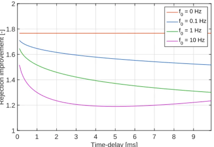
Figure 1: Improvement on variance reduction of predictor versus integrator (σ2
int/σ
2
min) for small time-delays and various values off0.
f
0∆t [-]
0 0.1 0.2 0.3 0.4 0.5 0.6 0.7
Normalised residual variance [-]
0 0.5 1 1.5
2 Optimal predictor Integrator
Figure 2: Normalised residual phase variancesσ2
min/σ
2
primandσ
2
int/σ
2
primagainstf0∆t.
f
0∆t [-]
0 0.05 0.1 0.15
Normalised residual variance [-]
0 0.2 0.4 0.6 0.8 1
Optimal predictor Integrator
Figure 3: Normalised residual phase variancesσ2
min/σ2primandσ2int/σ2primagainst small values off0∆t.
7
Analysis
The optimal predictor (14) is a function of time-delay∆t, wind speedvand outer scaleL0. It does not depend on for
instance the wavenumberk, zenith angleζor the index-of-refraction structure constantC2
From (7), (16) and (18) it follows that the minimum of the mean square time-delay error increases with ∆t and decreases withf0. Similar to the primary variance and the residual phase variance with the integrator, the
mini-mum variance grows with the5/3power of the Greenwood frequency. In addition, the normalised residual variance (σ2
res/σ
2
prim) is a function of the productf0∆t, for both the optimal predictor and the integrator.
The optimal predictor always performs better than the integrator; see Figures 1, 2 and 3. For small values off0∆t, the
improvement on phase variance reduction ranges from a factor 1.19 (forf0∆t= 0.05) up to 1.77 forf0∆t= 0, which
represents the Kolmogorov turbulence case. For largef0∆t, the optimal predictor becomes ineffective and achieves
no phase error reduction (forf0∆t > 0.4) . For the integrator, a largef0∆tvalue (>0.75) leads to doubling of the
primary variance, as phase disturbance values large∆t apart are fully uncorrelated; see Figure 2. Note, that these largef0∆tvalues are unlikely in practical cases.
Apart from a smaller temporal wavefront error, another benefit of optimal prediction in AO systems would be to allow for a longer detector integration time and therefore the use of a fainter reference star. Equalising the expressions for the residual variance, (21) and (22) for the Kolmogorov case, gives the following relation between the delay times:
∆topt= Γ(4
3)Γ( 1 6)
223√π
3 5
∆tint≈1.41∆tint (23)
So the detector integration time with an optimal predictor can be 1.41 times longer compared to the integrator case. This would allow a higher reference star magnitude and would improve the sky coverage.
Frequency [Hz]
10-2 10-1 100 101 102 103
Magnitude [-]
10-3 10-2 10-1 100
∆t = 1 ms
∆t = 3 ms
∆t = 10 ms
Figure 4: Optimal predictor sensitivity function forf0= 1 Hz and various values of∆t.
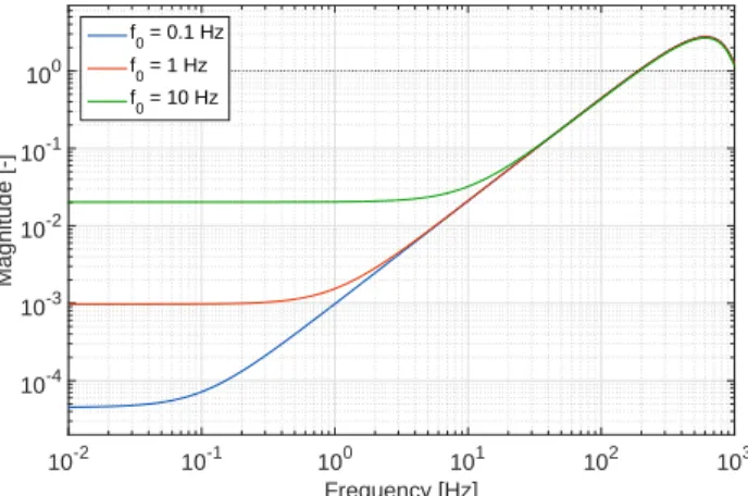
Frequency [Hz]
10-2 10-1 100 101 102 103
Magnitude [-]
10-4 10-3 10-2 10-1 100
f
0 = 0.1 Hz
f
0 = 1 Hz
f
0 = 10 Hz
Figure 5: Optimal predictor sensitivity function for∆t= 1 ms and various values off0.
The spectral behaviour of optimal prediction is shown in Figures 4 and 5, which reveal the modulus of the transfer function from input phase error to residual error (i.e. the sensitivity function). Figure 4 shows that the bandwidth of rejection reduces with the time-delay. The sensitivity curve crosses the unity magnitude line at approximately
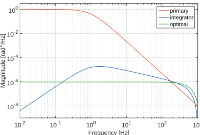
Frequency [Hz]
10-2 10-1 100 101 102 103
Magnitude [rad
2/Hz]
10-8 10-6 10-4 10-2
100 primary
integrator optimal
Figure 6: Power Spectral Density of phase fluctuations for the uncorrected case, the integrator and the optimal predictor for∆t= 1 ms andf0= 1 Hz.
degree of low-frequency attenuation is affected byf0; see Figure 5. In terms of the PSD of residual phase fluctuations
the optimal predictor achieves a flat spectrum over a large frequency band. It outperforms the integrator in the mid-frequency range, whereas the integrator obtains a higher low-mid-frequency rejection; see Figure 6. Both approaches have about the same frequency bandwidth of rejection and give rise to an increase of the high-frequency phase error.
8
Path-integrated turbulence
So far the analysis of residual wavefront errors has been restricted to propagation through a single, thin layer of turbulence. The atmosphere for the overall propagation path can be viewed as built up from multiple turbulent layers at different heights. For a plane wave and under the geometrical optics approximation, the path-integrated power spectrum of wavefront phase fluctuationsΦ(ω)can then be written as ([2]):
Φ(ω) =4 3
√
πΓ(7 6)k
2
Z
L dz C2
n(z)
v53(z)
(ω2+ω2 0(z))
4 3
(24)
Here, the PSD cut-off frequencyω0is a function of height, since both the outer scaleL0and the wind vectorvare
height-dependent. In fact, each turbulent layer has its own, specific PSD cut-off frequency. This prevents getting a similar compact form for the overall power spectrum as in (2) for a single layer. Following the approach proposed by several authors ([3, 2, 10]), an effective cut-off frequencyω0could be used instead. Theω0value is then set such
as to minimise the discrepancy between the true and approximated power spectrum for instance. This metric can be quantified as:
ǫ(ωc) =
∞
Z
−∞
dωΦ(ω, ωc) − Φ(ω)
2
(25)
whereΦ(ω, ωc)isΦ(ω)of eq. (24) withω0(z)replaced by the constantωc. The optimal value ofωcfor whichǫ(ωc) is minimised is denoted asω0. With the optimal value of the effective cut-off frequency in place, the path-integrated
wavefront phase (24) PSD becomes:
Φ(ω) = (2πfG)
5 3
ω2+ω 02
4 3
(26)
This power spectrum has exactly the same form as for the single layer case (5). And therefore, the full performance analysis of optimal and integrator prediction (section 7) also holds for the approximated path-integrated case with multiple turbulent layers. Note that for Kolmogorov turbulence specifically, the results section 7 are still exact as then the cut-off frequencyω0plays no role.
9
Conclusion
performance gain of optimal prediction can be significant. In more detail, the gain depends on the product of time-delay, wind speed and the reciprocal of outer scalev∆t/L0. The largest performance advantage is obtained for small
values ofv∆t/L0(<10−3). For larger values – up tov∆t/L0= 0.2– the performance gain is modest.
The analysis has been focused on wavefront phase prediction in an open-loop setting. Closed-loop aspects have not been taken into account. On the other hand, further reduction of the time-delay error could be achieved when accounting for the spatial properties of frozen flow. If Taylor’s hypothesis of frozen flow is valid, then wind-upstream sensor nodes would contain information of the future wavefront phase at wind-downstream sensor nodes. This enables the use of a feedforward-type prediction filter structure, leading to a higher reduction of the time-delay error (except for the sensor nodes at the upstream edge).
References
[1] David L Fried. Time-delay-induced mean-square error in adaptive optics.JOSA A, 7(7):1224–1225, 1990. [2] Larry C Andrews and Ronald L Phillips. Laser beam propagation through random media, volume 152. SPIE
press Bellingham, WA, 2005.
[3] Rodolphe Conan. Mean-square residual error of a wavefront after propagation through atmospheric turbulence and after correction with zernike polynomials.JOSA A, 25(2):526–536, 2008.
[4] Izrail Solomonovich Gradshteyn and Iosif Moiseevich Ryzhik.Table of integrals, series, and products. Academic press, 2007.
[5] Darryl P Greenwood. Bandwidth specification for adaptive optics systems.JOSA, 67(3):390–393, 1977. [6] Athanasios Papoulis and S Unnikrishna Pillai. Probability, random variables, and stochastic processes.Mc-Graw
Hill, 1991.
[7] Bertil Matérn. Spatial Variation: Stochastic Models and Their Application to Some Problems in Forest Surveys and Other Sampling Investigations. Statens skogsforskningsinstitut, 1960.
[8] Mark M Meerschaert, Farzad Sabzikar, Mantha S Phanikumar, and Aklilu Zeleke. Tempered fractional time series model for turbulence in geophysical flows. Journal of Statistical Mechanics: Theory and Experiment, 2014(9):P09023, 2014.
[9] John W Hardy.Adaptive optics for astronomical telescopes, volume 16. Oxford University Press, 1998. [10] VP Lukin, EV Nosov, and BV Fortes. The efficient outer scale of atmospheric turbulence. InEuropean Southern