Utilization of Long Columns Packed with Sub-2 μm Particles Operated at High Pressures and Elevated Temperatures for High-Efficiency One-Dimensional Liquid
Chromatographic Separations
Edward Gordon Franklin
A dissertation submitted to the faculty of the University of North Carolina at Chapel Hill in partial fulfillment of the requirements for the degree of Doctor of Philosophy in the
Department of Chemistry.
Chapel Hill 2012
Approved by:
Dr. James W. Jorgenson
Dr. Mark H. Schoenfisch
© 2012
ABSTRACT
EDWARD GORDON FRANKLIN: Utilization of Long Columns Packed with Sub-2 μm Particles Operated at High Pressures and Elevated Temperatures for High-Efficiency
One-Dimensional Liquid Chromatographic Separations (Under the direction of James W. Jorgenson)
As Ultrahigh Pressure Liquid Chromatography (UHPLC) techniques have become
increasingly popular across a number of scientific disciplines, the strongest emphasis has
remained on its ability to yield moderately high separation efficiencies on much faster
timescales than were previously achievable. This has been accomplished through the use of
commercial instrumentation capable of generating maximum pressures of 18,000 psi and 15
– 25 cm columns packed with 1.8 – 2.0 μm particles, providing theoretical plate counts
upwards of 60,000. While this represents a major step forward when compared to typical
HPLC approaches, many applications involving highly complex samples, such as those
encountered in “-omics” settings, stand to benefit from even higher efficiency separations.
The work presented in this dissertation explores the combined benefits of using
ultrahigh pressures (up to 50,000 psi), small particles (sub-2 μm) and elevated temperatures
(up to 85°C). Efforts were made to improve microcapillary column packing procedures by
investigating the individual and synergistic effects of experimental packing parameters on
ultimate column performance. Findings were used to pursue two of the most enduring
were used to pack columns several meters in length to achieve very high separation
efficiencies. A 360 cm x 50 μm ID column produced over 106 plates with a column dead
time of just over 100 minutes at 25°C. Likewise, ~ 200 cm columns were used in the
analyses of proteomic samples under gradient elution conditions to generate peak capacities
approaching 1000 in just over three hours at 65°. These results suggest a real applicability of
ACKNOWLEDGEMENTS
I would first like to thank my advisor, Dr. Jorgenson, under whom I have had the
privilege of working and studying for the past five years. His intellectual brilliance and
enthusiasm for research are truly remarkable. Through his guidance I have found much
encouragement for the completion of the work contained in this dissertation. Funding,
materials, and instrumentation for this work were provided by Waters Corporation. Also
with regard to this work, I must thank fellow graduate students Jordan Stobaugh and Kaitie
Fague. Without them, Chapter 5 would not exist. Thanks must also be given to many other
former and current Jorgenson Group members. They made the lab a great place to work, and
I am happy and blessed to call so many of them friends. Finally, I must thank my mother and
TABLE OF CONTENTS
LIST OF FIGURES ... xi
LIST OF ABBREVIATIONS ... xxii
LIST OF SYMBOLS... xxiv
CHAPTER 1: THEORY AND BACKGROUND ... 1
1.1 Overview ... 1
1.2 Chromatographic Theory ... 3
1.2.1 Chromatographic Separations ... 3
1.2.2 Separation Efficiency ... 4
1.2.3 Van Deemter Theory ... 6
1.2.3.1 A-term ... 8
1.2.3.2 B-term ... 13
1.2.3.3 C-term ... 14
1.2.4 Corrected Interstitial Velocities ... 17
1.2.5 Ultrahigh Pressure Liquid Chromatography (UHPLC) ... 18
1.2.5.1 UHPLC Pressures, Mobile Phase Viscosities, and Diffusion Coefficients ... 19
1.2.7 Kinetic Plots ... 20
1.3 References ... 22
1.4 Figures... 23
CHAPTER 2: INVESTIGATIONS AND IMPROVEMENTS OF MICROCAPILLARY COLUMN PACKING AND PERFORMANCE ... 30
2.1 Introduction ... 30
2.1.2 Bed Morphology and Its Influence on Chromatographic Performance ... 31
2.1.3 Experimental Packing Conditions for Producing Desired Bed Morphologies... 33
2.2 Experimental ... 37
2.2.1 Chemicals ... 37
2.2.2 General Capillary Column Packing Procedure ... 38
2.2.3 Column Evaluation ... 39
2.2.4 Segmented Column Performance ... 40
2.2.5 Column Outlet Effect ... 45
2.2.6 Slurry Concentration Effects ... 47
2.2.7 The Effect of Packing and Flushing Pressure... 52
2.2.8 Effect of Slurry Solvent ... 56
2.3 Conclusions ... 58
2.4 References ... 60
2.5 Figures... 62
CHAPTER 3: USE OF 1.0 MICRON-SIZED PACKING FOR FAST ANALYSES IN ULTRA HIGH PRESSURE CAPILLARY LIQUID CHROMATOGRAPHY ... 92
3.1 Introduction ... 92
3.1.1 Alternative Approaches to Fast, Efficient Liquid Chromatographic Separations ... 92
3.1.2 Theoretical Utility of 1.0 μm Porous Particle Supports ... 94
3.1.3 Previous Efforts with 1.0 μm Porous Particles ... 97
3.2.3 Effect of Slurry Concentration in Packing 1.5 and 1.0 μm Porous Particles ... 102
3.2.4 Effect of Column ID on Performance of Columns Packed with 1.5 and 1.0 μm Particles ... 103
3.2.5 Effect of Packing Pressure on Performance of Columns Packed with 1.0 μm Particles ... 104
3.2.5 Evaluation of 10 μm ID Columns Packed with 1.9, 1.5, and 1.0 μm Porous Particles ... 105
3.3 Conclusions ... 108
3.4 References ... 111
3.5 Figures... 112
CHAPTER 4: LONG MICROCAPILLARY COLUMNS AT ELEVATED TEMPERATURE AND PRESSURE FOR HIGH-EFFICIENCY ONE-DIMENSIONAL SEPARATIONS ... 129
4.1 Introduction ... 129
4.1.1 Survey of High-Efficiency Packed-Column Liquid Chromatography Separations ... 129
4.1.2 Alternative Means of Achieving High Separation Efficiency in Liquid Chromatography ... 131
4.1.2.1 Multidimensional Separations ... 131
4.1.2.2 Superficially Porous Particles ... 131
4.1.2.3 Porous Layer Open Tubular (PLOT) Columns... 132
4.1.2.4 Monolithic Columns... 133
4.1.2.5 Micropillar Array Columns (PACs) ... 133
4.1.3 Temperature as a Parameter in Liquid Chromatography ... 134
4.1.3.1 The Effect of Elevated Temperature on Column Efficiency ... 135
4.1.4 Kinetic Plots: The Combined Effects of Small Particles, High Pressures,
and Elevated Temperatures ... 137
4.1.5 Peak Capacity in Gradient Elution of Peptides ... 138
4.2 Experimental ... 141
4.2.1 Chemicals ... 141
4.2.2 Isocratic Characterization at Elevated Temperatures ... 142
4.2.3 100 cm Microcapillary Columns ... 144
4.2.3.1 Column ID Effects ... 145
4.2.3.2 Gradient Elution Characterization of 100 cm Microcapillary Columns ... 146
4.2.3.3 Slurry Concentration Effects ... 150
4.2.4 200 cm Microcapillary Columns ... 151
4.2.5 > 200 cm Mircrocapillary Columns ... 153
4.3 Conclusions ... 159
4.4 References ... 160
4.5 Figures... 162
CHAPTER 5: CONSTANT PRESSURE GRADIENT-CAPABLE PLATFORM FOR HIGH-EFFICIENCY ONE-DIMENSIONAL UHPLC SEPARATIONS ... 199
5.1 Introduction ... 199
5.1.1 Previous UHPLC Gradient System ... 199
5.1.2 Conceptual Features of New Gradient UHPLC System ... 201
5.2 System Design and General Operation ... 203
5.3.3 Results with Direct Injection ... 210
5.4 Conclusions ... 213
5.5 Figures... 215
LIST OF FIGURES
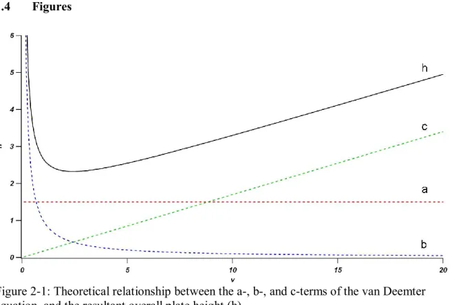
Figure 1-1: Theoretical relationship between the a-, b-, and c-terms of the van
Deemter equation, and the resultant overall plate height (h) ... 23
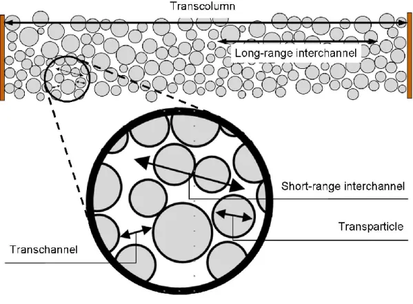
Figure 1-2: Categorical distances of the five contributors to eddy diffusion identified
by Giddings. Figure adapted from Ref. 6. ... 24
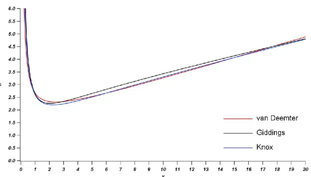
Figure 1-3: Overlay of the reduced forms of the van Deemter, Giddings, and Knox
equations with typical values for the coefficients. ... 25
Figure 1-4: Mobile phase velocities experimentally determined from a dead time marker can be corrected to account for intraparticle stagnant mobile phase to find approximate interstitial velocities. The corrected interstitial velocities should be used
in constructing van Deemter curves. ... 26
Figure 1-5: The mechanism of hydrodynamic flow chromatography (HDC) in a channel. Large particles cannot adequately sample the slowest flow regimes at the walls, and measuring their elution times results in overestimating the actual interstitial
velocity. ... 27
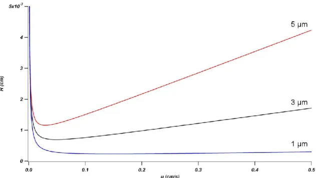
Figure 1-6: The effect of decreasing particle diameter on column performance. ... 28
Figure 1-7: Kinetic plots for 1, 3, and 5 μm particles. ∆P = 400 bar (~5800 psi);
viscosity, η = 1 cP; interparticle porosity, εi = 0.4; diffusion coefficient, Dm = 1 x 10⁻⁵
cm/s; reduced van Deemter coefficients A = 1.0, B = 1.0, and C = 0.1. ... 29
Figure 2-1: van Deemter curves of inlet and outlet halves of a bisected 100 cm x 50 μm ID column packed with ~ 10 mg/mL slurry of 1.9 μm BEH particles in acetone.
Data points are for the intact 100 cm column. ... 62
Figure 2-2: Overlaid van Deemter curves for all four ~ 25 cm segments of an originally 100 cm x 50 μm ID column packed with ~ 10 mg/mL slurry of 1.9 μm
BEH particles in acetone. ... 63
Figure 2-3: Resistance to flow data for all four ~ 25 cm segments of an originally 100 cm x 50 μm ID column packed with ~ 10 mg/mL slurry of 1.9 μm BEH particles in
acetone. ... 64
Figure 2-4: Retention data for all four ~ 25 cm segments of an originally 100 cm x 50
Figure 2-6: Replicate data of resistance to flow for all four ~ 25 cm segments of an originally 100 cm x 50 μm ID column packed with ~ 10 mg/mL slurry of 1.9 μm
BEH particles in acetone. ... 67
Figure 2-7: Replicate retention data for all four ~ 25 cm segments of an originally 100 cm x 50 μm ID column packed with ~ 10 mg/mL slurry of 1.9 μm BEH particles in
acetone. ... 68
Figure 2-8: Overlaid van Deemter curves from column where increasing lengths of column were clipped from the outlet end. A ~ 3 mg/mL slurry of BEH particles in
acetone was used to pack the original 50 cm x 50 μm ID column. ... 69
Figure 2-9: Overlaid van Deemter curves from column where increasing lengths of column were clipped from the outlet end. A ~ 100 mg/mL slurry of BEH particles in
acetone was used to pack the original 49 cm x 50 μm ID column. ... 70
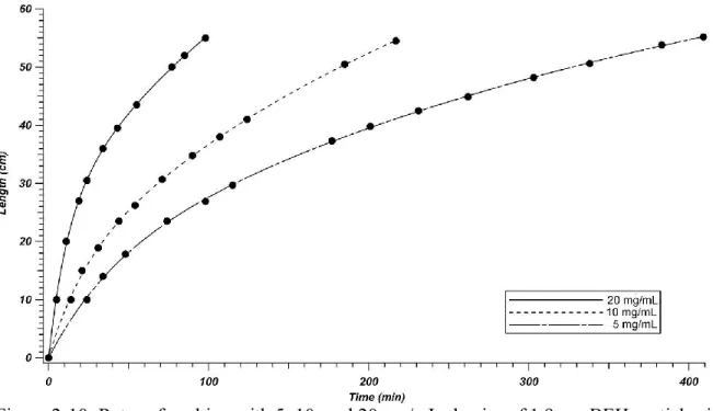
Figure 2-10: Rates of packing with 5, 10, and 20 mg/mL slurries of 1.9 μm BEH
particles in acetone. ... 71
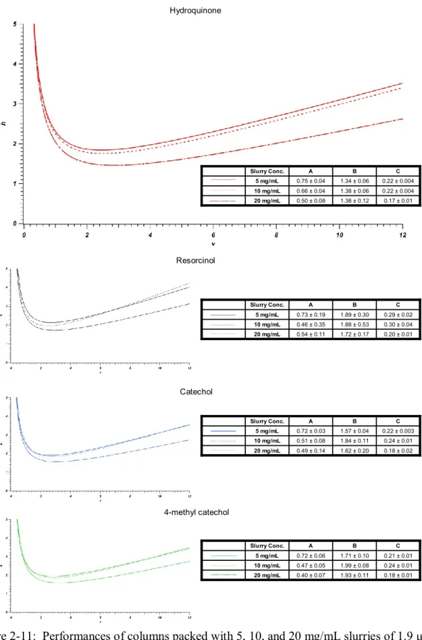
Figure 2-11: Performances of columns packed with 5, 10, and 20 mg/mL slurries of
1.9 μm BEH particles slurried in acetone. ... 72
Figure 2-12: Rates of packing with 100, 20, 10, and 5 mg/mL slurries of 1.9 μm BEH
particles in acetone. The 100 mg/mL slurry packing rate is highlighted in red... 73
Figure 2-13: Overlaid van Deemter curves for consecutively packed 50 μm ID
columns ... 74
Figure 2-14: Comparison of performances for ~ 25 cm x 75 μm ID columns packed
with 3 and 100 mg/mL slurries of 1.9 μm BEH particles. ... 75
Figure 2-15: Comparison of column retention for ~ 25 cm x 75 μm ID columns
packed with 3 and 100 mg/mL slurries of 1.9 μm BEH particles. ... 76
Figure 2-16: Comparison of column resistance to flow for ~ 25 cm x 75 μm ID
columns packed with 3 and 100 mg/mL slurries of 1.9 μm BEH particles. ... 77
Figure 2-17: Overlaid van Deemter curves for all four ~ 25 cm segments of an originally 100 cm x 50 μm ID column packed with ~ 100 mg/mL slurry of 1.9 μm
BEH particles in acetone. ... 78
Figure 2-18: Retention data for all four ~ 25 cm segments of an originally 100 cm x 50 μm ID column packed with ~ 100 mg/mL slurry of 1.9 μm BEH particles in
Figure 2-19: Resistance to flow data for all four ~ 25 cm segments of an originally 100 cm x 50 μm ID column packed with ~ 100 mg/mL slurry of 1.9 μm BEH
particles in acetone. ... 80
Figure 2-20: Overlaid van Deemter curves for permutations of ~ 25 cm columns packed at 10,000 or 30,000 psi and subsequently flushed at 23,000 or 46,000 psi.
Columns were packed with ~ 100 mg/mL of 1.9 μm BEH particles in acetone. ... 81
Figure 2-21: Retention data for permutations of ~ 25 cm columns packed at 10,000 or 30,000 psi and subsequently flushed at 23,000 or 46,000 psi. Columns were packed
with ~ 100 mg/mL of 1.9 μm BEH particles in acetone... 82
Figure 2-22: Resistance to flow data for permutations of ~ 25 cm columns packed at 10,000 or 30,000 psi and subsequently flushed at 23,000 or 46,000 psi. Columns
were packed with ~ 100 mg/mL of 1.9 μm BEH particles in acetone. ... 83
Figure 2-23: Overlaid van Deemter curves of ~ 25 cm column packed at 10,000 psi and flushed at 23,000 psi with a second column packed at 30,000 psi and flushed at
46,000 psi. ... 84
Figure 2-24: Retention data of ~ 25 cm column packed at 10,000 psi and flushed at 23,000 psi with a second ~ 25 cm column packed at 30,000 psi and flushed at 46,000
psi. ... 85
Figure 2-25: Resistance to flow data of ~ 25 cm column packed at 10,000 psi and flushed at 23,000 psi with a second column packed at 30,000 psi and flushed at
46,000 psi. ... 86
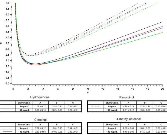
Figure 2-26: Performances of 50 μm ID columns packed with 3, 10, and 50, and 100
mg/mL slurries of 1.9 μm BEH particles in methanol. ... 87
Figure 2-27: Performances of 75 μm ID column packed with 50 mg/mL slurry of 1.9
μm BEH particles in methanol. ... 88
Figure 2-28: Performances of 75 μm ID column packed with 100 mg/mL slurry of
1.9 μm BEH particles in methanol. ... 89
Figure 2-29: Performances of 150 μm ID column packed with 100 mg/mL slurry of
1.9 μm BEH particles in methanol. ... 90
Figure 2-30: Performances of 150 μm ID column packed with 100 mg/mL slurry of
diffusion coefficient, Dm = 1 x 10⁻⁵ cm2/s; reduced van Deemter coefficients A = 1.5,
B = 1.0, and C = 0.17 ... 112
Figure 3-2: Expected performance of columns of various lengths packed with 1 μm particles operated at 15,000 psi (blue trace) and 40,000 psi (red trace) Plots are
constructed assuming viscosity, η = 1 cP; interparticle porosity, εi = 0.4; analyte
diffusion coefficient, Dm = 1 x 10⁻⁵ cm2/s; reduced van Deemter coefficients A = 1.5,
B = 1.0, and C = 0.17. ... 113
Figure 3-3: h vs. v plots for 19 cm x 30 μm ID column packed with 1.0 μm BEH particles run in 50/50 acetonitrile/water and 0.5% TFA. The sudden deterioration in
performance at higher linear velocities was caused by bed collapse. ... 114
Figure 3-4: Chromatogram of 20 cm x 30 μm ID column packed with 1.0 μm BEH
operated at 40,000 psi in 50/50 acetonitrile/water and 0.1% TFA... 115
Figure 3-5: van Deemter performance of a 20 cm x 30 μm ID column packed with
1.0 μm BEH particles run in 50/50 acetonitrile/water and 0.5% TFA. ... 116
Figure 3-6: Comparison of performances of 30 μm ID columns packed with 2
mg/mL (14.6 cm) and 20 mg/mL (15.1 cm) slurries of 1.0 μm BEH particles. ... 117
Figure 3-7: Comparison of column retention for ~ 15 cm x 30 μm ID columns packed with 2 (dashed lines) and 20 mg/mL (solid lines) slurries of 1.0 μm BEH
particles. ... 118
Figure 3-8: Comparison of column resistance to flow for ~ 15 cm x 30 μm ID columns packed with 2 (dashed line) and 20 (solid line) mg/mL slurries of 1.0 μm
BEH particles. ... 119
Figure 3-9: Comparison of performances of 25.4 cm x 50 μm ID columns packed
with 3 mg/mL and 30 mg/mL slurries of 1.5 μm BEH particles. ... 120
Figure 3-10: Comparison of column retention for 25.4 cm x 50 μm ID columns packed with 3 (dashed lines) and 30 mg/mL (solid lines) slurries of 1.5 μm BEH
particles. ... 121
Figure 3-11: Comparison of column resistance to flow for 25.4 cm x 30 μm ID columns packed with 3 (dashed line) and 30 (solid line) mg/mL slurries of 1.5 μm
BEH particles. ... 122
Figure 3-12: Effect of column inner diameter on chromatographic performance for columns packed with 1.5 μm BEH particles. Columns dimensions were 25.7 cm x 30
Figure 3-13: Effect of column inner diameter on chromatographic performance for columns packed with 1.0 μm BEH particles. Columns dimensions were 28 cm x 15
μm ID; 20 cm x 30 μm ID; 30.2 x 50 μm. ... 124
Figure 3-14: Effect of maximum packing pressure on chromatographic performance for columns packed with 1.0 μm BEH particles. Columns dimensions were 19.8 cm x
30 μm ID (10,000 psi); 20 cm x 30 μm ID (20,000 psi); and 20 x 30 μm (30,000 psi). ... 125
Figure 3-15: Performance of 10 μm ID columns packed with 1.0 μm BEH (14.3 cm),
1.5 μm BEH (26.3 cm), and 1.9 μm BEH (25.8 cm)... 126
Figure 3-16: Kinetic plots showing the performance of 1.0 vs. 1.9 μm particles with pressure limitations of 40,000 psi. Reduced van Deemter coefficients of A=0.30, B=2.06, and C=0.15 are used in the construction of the 1.9 μm curve (blue trace) and the theoretical 1.0 μm curve (dashed red trace). Reduced van Deemter coefficients of A=0.15, B=2.26, and C=0.27 are used in the construction of the 1.0 μm curve (red
trace). Plots are constructed assuming viscosity, η = 1 cP; interparticle porosity, εi =
0.4; analyte diffusion coefficient, Dm = 1 x 10⁻⁵ cm2/s. ... 127
Figure 3-17: Kinetic plots showing the performance of 1.0 μm particles with pressure limitations of 40,000 psi packed in 10 μm and 30 μm ID capillary. Reduced van Deemter coefficients of A=0.15, B=2.26, and C=0.27 are used in the construction of the 10 μm ID curve (red trace). Reduced van Deemter coefficients of A=0.03, B=2.41, and C=0.30 are used in the construction of the 30 μm ID curve (blue trace).
Plots are constructed assuming viscosity, η = 1 cP; interparticle porosity, εi = 0.4;
analyte diffusion coefficient, Dm = 1 x 10⁻⁵ cm2/s. ... 128
Figure 4-1: Theoretical H vs. U curves for 1.9 μm particles at 25, 45, 65, and 85°C, using reduced A-, B-, and C- terms of 1.5, 1.0, and 0.1, respectively. Mobile phase viscosities are calculated according to the Chen-Horvath equation, and diffusion
coefficients are scaled accordingly. ... 162
Figure 4-2: Series of theoretical curves representing the performance of 25 cm – 1000 cm columns. Curves are constructed using reduced van Deemter coefficients of 1.0, 1.0, and 0.1 for A-, B-, and C-, respectively. Mobile phase viscosities of 0.89 cP
and diffusion coefficients of 8.0 x 10⁻⁶ cm2/s are assumed. Each dead-time
corresponds to an operating pressure. The intersection of the red trace with the
curves shows expected performance when operating at 40,000 psi. ... 163
curve represents columns run at 25°C and 15,000 psi. The red trace highlights the increase in accessible efficiencies that become available when operating at 85°C and
40,000 psi. Each dead-time corresponds to a column length... 165
Figure 4-5: Peak capacity as a function of gradient time using Equation 4-10 for a 15 cm x 4.6 mm column with 5 μm particles and a fixed flow rate of 1.0 mL/min.
Theoretical plates are estimated using A=5dp, B=1Dm, and C=dp2/(6Dm). A diffusion
coefficient of 8.0 x 10⁻⁶ cm2/s is assumed. ... 166
Figure 4-6: Peak capacity as a function of flow rate for a 15 cm x 4.6 mm column packed with 5 μm particles. Gradient time is fixed at 1 hour. Maximum N as
determined by the van Deemter coefficients A=5dp, B=1Dm, and C=dp2/(6Dm) occurs
at a flow rate 8x slower than that which yields the highest peak capacity. ... 167
Figure 4-7: Peak capacity as a function of column flow rate for 15 cm x 4.6 mm columns. The solid trace is for 5 μm particles; the dashed trace is for 1.9 μm particles
Gradient time is fixed at 1 hour. ... 168
Figure 4-8: Experimental set-up for performing isocratic characterization at elevated temperatures. The majority of the column is housed within an aluminum heating block, held at temperature through feedback control of two heating cartridges. The first ~6 cm of column is unthermostatted within the column injector. 0.5 cm of column outlet protrudes from the heating block and is butt-connected to an open
capillary for electrochemical detection. ... 169
Figure 4-9: Chromatograms collected near optimum linear velocity for a 66 cm x 50 μm ID column packed with 1.9 μm BEH particles at 23, 45, 65, and 85°C in 50/50
acetonitrile/water and 0.1% TFA. ... 170
Figure 4-10: Overlaid reduced van Deemter curves for hydroquinone collected at 23,
45, 65, and 85°C for a 66 cm x 50 μm ID column packed with 1.9 μm BEH particles. ... 171
Figure 4-11: Modified experimental set-up for performing isocratic characterization at elevated temperatures. The majority of the column is housed within an aluminum heating block, held at temperature through feedback control of two heating cartridges. The injector is held at matching temperature using four heating cartridges.
Approximately 2 cm of column resides between the injector and heating block. 0.5 cm of column outlet protrudes from the heating block and is butt-connected to an
open capillary for electrochemical detection. ... 172
Figure 4-12: Chromatograms collected near optimum linear velocity for a 60 cm x 50 μm ID column packed with 1.9 μm BEH particles at 23, 45, 65, and 85°C using 30/70
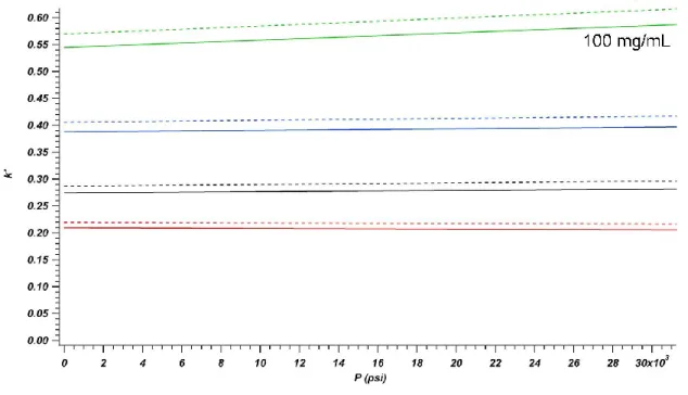
Figure 4-13: Retention as a function of operating pressure at 23, 45, 65, and 85°C for a 60 cm x 50 μm ID column packed with 1.9 μm BEH in 30/70 acetonitrile/water and
0.1% TFA. ... 174
Figure 4-14: Van’t Hoff plot of the retained test analytes at 23, 45, 65, and 85°C in
30/70 acetonitrile/water and 0.1% TFA. ... 175
Figure 4-15: H vs. U plots for hydroquinone at 23, 45, 65, and 85°C. Comparison
with theoretical predictions in Figure 4-1 reveals the expected increase in Uopt at
elevated temperatures and preserved column efficiency. ... 176
Figure 4-16: Overlay of reduced van Deemter plot for each analyte at 23, 45, 65, and 85°C. Reduced parameters at elevated temperatures are calculated from estimated pressure-dependent mobile phase viscosities and corresponding increases in analyte
diffusion coefficients. ... 177
Figure 4-17: Chromatograms highlighting the on-column oxidation of 4-methyl catechol. With longer analysis times, the peak is rendered electrochemically
undetectable. a) 33,000 psi; b) 18,000 psi; c) 12,000 psi. ... 178
Figure 4-18: Overlay of van Deemter performances for five ~100 cm x μm ID columns packed over a three month period. Experimental packing conditions were
virtually identical with particle slurry concentrations ranging between 5-10 mg/mL. ... 179
Figure 4-19: Effect of column inner diameter on performance of ~100 cm columns.
As observed in the past, performance improves dramatically with decreasing ID. ... 180
Figure 4-20: Schematic view of UHPLC gradient system. The gradient is generated by a Waters CapLC pump and loaded onto an external storage loop, followed by the sample. Flow resistances of the packed analytical column and small-ID flow splitter ensure that the vast majority of flow reaches the loop. Once the sample is loaded, both pin valves are closed, and the hydraulic amplifier is engaged to push the sample and gradient into the micro-volume cross. Much of the sample and gradient is diverted to waste through the flow splitter, while a small volume makes it onto the
analytical column for analysis. ... 181
Figure 4-21: Representative chromatograms of a tryptic digest of bovine serum albumin run in 1-50% acetonitrile gradients corresponding to total run times of 60, 120, 180, and 240 minutes. Runs were performed on a 100 cm x 50 μm ID column packed with 1.9 μm BEH particles. Operating pressure was ~ 24,000 psi, but varied throughout the runs with changing mobile phase viscosities. Mass spectrometric
widths of representative peaks in 1-50% acetonitrile gradients for a BSA tryptic
digest sample. ... 183
Figure 4-23: Peak capacity vs. retention window for a 100 cm x 30 μm ID column packed with 1.9 μm particles. 1-50% acetonitrile gradients for a BSA tryptic digest sample were run and peak capacities determined from 4σ base widths of
representative peaks. Retention windows were determined from the elution times of two characteristic peaks, and peak capacities calculated by dividing the retention
window by the average peak width. ... 184
Figure 4-24: Peak capacity vs. mobile phase linear velocity as determined by the column dead time for four gradient steepnesses, represented by % change of mobile
phase composition per column volume. ... 185
Figure 4-25: Representative chromatograms of a) 105 cm and b) 103 cm x 50 μm ID
columns packed with a 100 mg/mL slurry of 1.9 μm BEH particles. ... 186
Figure 4-26: Reduced van Deemter curves of the consecutively packed 105 cm and
103 cm x 50 μm ID columns packed with 100 mg/mL slurries of 1.9 μm BEH. ... 187
Figure 4-27: Retention data for the consecutively packed 105 (solid trace) cm and
103 cm (dashed trace) columns, highlighting the similarity of column permeability. ... 188
Figure 4-28: Flow resistances of the consecutively packed 105 cm (solid trace) and
103 cm (dashed trace) columns. ... 189
Figure 4-29: Chromatograms collected at 25°C and 65°C for a 180 cm x 50 μm ID
column operated at 45,000 psi. ... 190
Figure 4-30: h vs. v plots of the 180 cm x 50 μm ID column. 4-methyl catechol is
oxidized on-column at 65 °C. ... 191
Figure 4-31: Representative chromatogram of a 214 cm x 50 μm ID column packed with a 100 mg/mL slurry of 1.9 μm BEH particles, operated at 38,500 psi. The improved performance when packing with concentrated slurries is reflected in the
number of theoretical plates. ... 192
Figure 4-32: Chromatograms and determined peak capacities for a 216 cm x 50 μm ID column packed with 1.9 μm BEH. 1-50% acetonitrile gradients of 120, 240, and 360 minutes for a BSA tryptic digest sample were run and peak capacities determined
from 4σ base widths of representative peaks. ... 193
two characteristic peaks, and peak capacities calculated by dividing the retention
window by the average peak width. ... 194
Figure 4-34: Overlaid h vs. v data for the first (closed markers) and last packed (open
markers) ~ 100 cm segments of a originally 330 cm x 50 μm ID column packed with 1.9 μm BEH particles. Data highlighted in the red circle shows deteriorated
performance subsequent to collected data at the highest operating pressures, signaling
packed bed instability. ... 195
Figure 4-35: Overlaid reduced van Deemter plots of 100 cm x 50 μm ID columns packed at 30,000 psi and subsequently flushed at either 23,000 psi or 50,000 psi. The
column flushed at 50,000 psi performs superiorly. ... 196
Figure 4-36: Modified UHPLC compression fitting to allow for the zero dead-volume connection of two microcapillary columns in series. The body is machined from 17-4 PH stainless steel, the compression bolt from 316 stainless steel, and the stem from D-2 air hardened tool steel. Capillary columns are abutted in the center of the PEEK ferrule and compression serves to grip the columns axially without twisting
the silica faces over one another, thereby preventing breakage. ... 197
Figure 4-37: Chromatograms collected at a) 40,000 psi and b) 45,000 psi of a 360 cm x 50 μm ID column packed with 1.9 μm BEH particles. Total column length was achieved by the series connection of a 190 cm and 170 cm column in the compression
fitting shown in Figure 4-36. ... 198
Figure 5-1: Chromatograms of a yeast cell lysate digest. a) A 90 minute 5-40% acetonitrile gradient performed on a commercial 25 cm x 75 μm ID packed with 1.9 μm BEH particles at 40°C; b) A 6 hour 1-50% acetonitrile gradient performed on a 200 cm x 50 μm ID column packed with 1.9 μm BEH at 25°C; c) An ~ 100 minute expanded view of the separation in (b); d) The same gradient utilized in (b) played
back at 65°C. ... 215
Figure 5-2: Viscosity as a function of acetonitrile/water composition according to the
Chen-Horvath equation shown in Equation 5-1 at 25, 45, 65, and 85°C. ... 216
Figure 5-3: Viscosity as a function of acetonitrile/water composition according to the Chen-Horvath equation shown in Equation 5-1 at 25, 45, 65, and 85°C. The data is normalized to the highest viscosity at each temperature to highlight the % change
through 0-50% acetonitrile. ... 217
Figure 5-4: Schematic of the modified instrumentation to perform constant pressure
Figure 5-6: Sample trapping scheme: Pin valves 1, 3, and 4 are closed. Pin valves 2
and 5 are open to allow flow from the nanoAcquity through the trap column to waste. ... 220
Figure 5-7: Gradient playback at UHPLC pressures: Pin valves 2, 4, and 5 are closed. Pin valve 3 is open, and engagement of the Haskel pump pushes the gradient from the storage loop onto the trap and analytical columns. Pin valve 1 is open to allow flow from the nanoAcquity to ramp down and to divert flow away from the commercial
instrument should Pin valve 2 fail during operation. ... 221
Figure 5-8: Theoretical plates vs. dead times for 50 – 400 cm columns packed with 1.9 μm particles, operated at 65°C. The intersection of the red trace with the curves shows expected performance when operating at 30,000 psi. Curves are constructed using reduced van Deemter coefficients of 1.0, 1.0, and 0.1 for A-, B-, and C-, respectively. Mobile phase viscosities of 0.48 cP and diffusion coefficients of 1.7 x
10-5 cm2/s are assumed. ... 222
Figure 5-9: Theoretical plates vs. dead times for 25 – 200 cm columns packed with 1.5 μm particles, operated at 65°C. The intersection of the red trace with the curves shows expected performance when operating at 30,000 psi. Curves are constructed using reduced van Deemter coefficients of 1.0, 1.0, and 0.1 for A-, B-, and C-, respectively. Mobile phase viscosities of 0.48 cP and diffusion coefficients of 1.7 x
10-5 cm2/s are assumed. ... 223
Figure 5-10: Theoretical plates vs. dead times for 25 – 200 cm columns packed with 1.0 μm particles, operated at 65°C. The intersection of the red trace with the curves shows expected performance when operating at 30,000 psi. Curves are constructed using reduced van Deemter coefficients of 1.0, 1.0, and 0.1 for A-, B-, and C-, respectively. Mobile phase viscosities of 0.48 cP and diffusion coefficients of 1.7 x
10-5 cm2/s are assumed. ... 224
Figure 5-11: Separation of a yeast cell lysate on a 200 cm x 75 μm ID column packed with 1.9 μm BEH particles at 30,000 psi and 65°C using a 35 μL gradient of 4-40%
acetonitrile. ... 225
Figure 5-12: Peak tailing as evidenced by five single ion chromatograms from 139-144 minutes for the separation of a yeast cell lysate on a 200 cm x 75 μm ID column packed with 1.9 μm BEH particles at 30,000 psi and 65°C using a 35 μL gradient of
4-40% acetonitrile. ... 226
Figure 5-13: Separations of a yeast cell lysate on 75 μm ID columns packed with 1.5 μm BEH particles at 30,000 psi and 65°C. a) 117 cm column, 25 μL gradient of 3-40% acetonitrile; b) 117 cm column, 45 μL gradient of 3-3-40% acetonitrile; c) 100 cm
column, 85 μL gradient of 1-40% acetonitrile. ... 227
packed with 1.5 μm BEH particles at 30,000 psi and 65°C using a 85 μL gradient of
1-40% acetonitrile. ... 228
Figure 5-15: Separations of a yeast cell lysate on a 25 cm x 75 μm ID column packed with 1.0 μm BEH particles at 30,000 psi and 65°C using 1-40% acetonitrile gradients.
a) 15 μL gradient; b) 25 μL gradient; c) 35 μL gradient. ... 229
Figure 5-16: Peak capacity vs. retention window plot comparing the performances of a commercial 25 cm x 75 μm ID column packed with 1.9 μm BEH particles (black)
and a 25 cm x 75 μm ID column packed with 1.0 μm BEH particles (red). ... 230
Figure 5-17: Schematic of the modified instrumentation to perform constant pressure
gradient UHPLC separations with direct sample injections. ... 231
Figure 5-18: Gradient and sample loading scheme in direct injection mode: Pin valve 1 is closed. Pin valves 2 and 4 are open to allow flow from the nanoAcquity to the
gradient storage loop. ... 232
Figure 5-19: Gradient playback at UHPLC pressures in direction mode: Pin valves 2 and 4 are closed. Engagement of the Haskel pump pushes the sample and gradient from the storage loop onto the analytical column. Pin valve 1 is open to allow flow from the nanoAcquity to ramp down and to divert flow away from the commercial
instrument should Pin valve 2 fail during operation. ... 233
Figure 5-20: Separations of an E.coli digestion standard using a 100 cm x 75 μm ID column packed with 1.5 μm BEH particles in direct injection mode at 30,000 psi and 65°C with 1-40% acetonitrile gradients with total volumes of: a) 25 μL; b) 50 μL; c)
100 μL; d) 150 μL; e) 200 μL. ... 234
Figure 5-21: Peak capacity vs. retention window plot showing the performance of a 100 cm x 75 μm ID column packed with 1.5 μm BEH particles operated at 30,000 psi
and 65°C in direct injection mode. ... 235
Figure 5-22: Improved peak shape as evidenced by five single ion chromatograms from 57-60 minutes for the separation of an E.coli digestion standard on a 100 cm x 75 μm ID column packed with 1.5 μm BEH particles at 30,000 psi and 65°C using a
100 μL gradient of 1-40% acetonitrile in direct injection mode. ... 236
LIST OF ABBREVIATIONS
2D-LC two-dimensional liquid chromatography
BEH ethylene Bridged Hybrid
BSA bovine serum albumin
C18 n-octadecyl
CEC capillary electrochromatography
CLSM confocal laser scanning microscopy
EMT effective medium theory
ESI electrospray ionization
HDC hydrodynamic chromatography
HETP height equivalent of a theoretical plate
HPLC high performance liquid chromatography
ID inner diameter
ISEC inverse size exclusion chromatography
LC liquid chromatography
MEK methyl ethyl ketone
MS mass spectrometry
MS/MS tandem mass spectrometry
PAC micropillar array column
PEEK polyether ether ketone
PLOT porous-layer open tubular
PSD particle size distribution
RSD relative standard deviation
TFA trifluoracetic acid
THF Tetrahydrofuran
TOF time-of-flight
LIST OF SYMBOLS
Fraction of mobile phase contained inside pores
p
Volume fraction of particles
w Average peak width
∆c Change in solvent composition over the course of the gradient
∆H0 System enthalpy
∆P Change in pressure
∆Popt Pressure needed to obtain optimum flow rate/mobile phase linear velocity
∆S0 System entropy
A Eddy dispersion van Deemter coefficient
ASP Specific surface area
B Longitudinal diffusion van Deemter coefficient
C Resistance to mass transfer van Deemter coefficient
CM Concentration of analyte in mobile phase
CS Concentration of analyte in stationary phase
DA,B Diffusion coefficient of solute A infinitely diluted in solvent B
dc Column diameter
Deff Effective diffusion coefficient
DM Diffusion coefficient of analyte in mobile phase
Dms Diffusion coefficient inside porous particle
dp Particle diameter
Ds Diffusion coefficient in the stationary phase
F Flow
g Gravitational constant
G Gradient steepness factor
H Height equivalent of a theoretical plate
h Reduced plate height
HA Height equivalent to a theoretical plate due to eddy dispersion
HB Height equivalent to a theoretical plate due to longitudinal diffusion
HC Height equivalent to a theoretical plate due to resistance to mass
Transfer
HCM Constribution to HC occurring in the mobile phase
HCS Constribution to HC occurring in the stationary phase
HCSM Constribution to HC occurring in stagnant mobile phase
Hheat Heat of friction contribution to theoretical plate height
hmin Minimum reduced plate height
K Partition coefficient
k Boltzman constant
k’ Retention factor
K2 Particle-solvent dependent constant
L Column length
MB Molecular weight of solvent B
N Number of theoretical plates
nM Number of moles in mobile phase
nS Number of moles in stationary phase
r Radius of packed bed
R Universal gas constant
rH Hydrodynamic radius of solute
Rs Specific resolution
S Distance traveled by analyte molecule in a given flow path
Sk’ Slope of the plot of the natural logarithm of the retention factor versus
solvent composition
T Absolute temperature
te Time to transfer analyte molecule from on velocity extreme to another
tg Gradient run time
tM Time analyte spends in mobile phase
tm Column dead time
tR Retention time
tS Time analyte spends in stationary phase
u Mobile phase linear velocity
ui Interstitial velocity
v Reduced velocity
VA Molecular volume of solute A at normal boiling temperature
VM Volume of mobile phase
vopt Optimum reduced velocity
VP,0 Peak volume with very small injection volume
VR Retention volume
VS Volume of stationary phase
vs Sedimentation velocity
VS Sample injection volume
VSP Specific pore volume
x Mole fraction
α Selectivity factor
β Phase ratio
γ Tortuosity factor
εf Particle porosity filled with mobile phase
εi Volume fraction of interstitial spaces
εp Particle porosity
εt Volume fraction of column occupied by mobile phase
η Mobile phase viscosity
λ Scaling factor associated with the structure of the packed bed
ρl Solvent density
ρskel Particle skeleton density
σL2 Spatial variance
σt2 Temporal variance
ω Flow resistance factor
ωα Fractional value of the particle diameter traveled to get from one velocity
extreme to another
ωβ Velocity ratio defined by ∆u/u, where ∆u is the difference between the
CHAPTER 1: THEORY AND BACKGROUND 1.1 Overview
In attempting to improve the majority of liquid chromatographic separations, it is
generally regarded that selectivity factor (α) plays a more significant role than the column
efficiency parameter (N), as illustrated by Equation 1-1, an approximate expression for peak
resolution (Rs)1.
N α 1 α ) k' 1 ( k' 4 1
Rs
(1-1)
where k’ is the retention factor of the first peak. A notable exception to this rule is in the
analysis of complex samples containing many components. In such instances,
high-efficiency use of the entire separation space is often more important than the critical
resolution of any two specific peaks. The two principal means of achieving higher
efficiencies in liquid chromatography are reducing particle size (dp) and increasing column
length (L). In either of these approaches, the efficiency limit that can be achieved is dictated
by the pressure drop across the column. Thus, instrumentation (i.e. pumping capabilities)
becomes a key limiting factor in the maximization of separation efficiency.
Typical High Performance Liquid Chromatography (HPLC) instrumentation is
capable of generating pressures up to 6,000 psi. As such, researchers are generally restricted
particles at higher pressures, and by the late 1990s, they had demonstrated these
improvements with what was termed Ultrahigh Pressure Liquid Chromatography (UHPLC).
The technique utilized fused silica capillary columns packed with sub-2 μm nonporous silica
particles and operating pressures as high as 100,000 psi to generate plate numbers upwards of
300,000 in under 6 minutes2,3.
More than a decade later, commercialization of technologies commensurable with
UHPLC performances has not been realized. Nonetheless, significant strides were taken
when Waters Corporation (Milford, MA) began marketing instrumentation (Acquity) capable
of operating at 15,000 psi for use with 15 cm columns packed with 1.7 μm particles. Other
manufacturers quickly followed suit with high pressure hardware: Agilent (the 1200 series)
Thermo Fisher (Accela), Jasco (Xtreme-LC), Shimadzu (UFLC-XR), Hitachi (LaChrom
Ultra), Scientific Systems (Ultra HP), Dionex (RSLC), Knauer (Platin Blue), and
PerkinElmer (Flexar). The general marketing strategy for these higher pressure systems has
emphasized the speed of analysis and the long-term cost savings as it relates to decreased
solvent consumption. However, using the technology to push the limits of high-efficiency
one-dimensional separations remains a relatively under-sampled endeavor.
The work presented in this thesis focuses on harnessing the combined benefits
provided by ultrahigh pressures, small particle diameters, and elevated temperatures to
achieve very high efficiency separations on time-scales that are much more manageable than
those previously reported. The remainder of this introductory chapter will lay the theoretical
groundwork needed to understand chromatographic theory and the relevant aspects of
UHPLC toward this goal. Chapter 2 discusses general features of the microcapillary column
insights gained through investigating them. Chapter 3 specifically discusses the use of 1 μm
fully porous particles in UHPLC, their utility, and strides made with regard to improving the
efficiencies of columns packed with these materials. Chapter 4 describes the performance
characteristics of capillary columns packed in excess of 1 meter under both isocratic and
gradient elution conditions. Finally, Chapter 5 describes a new UHPLC gradient-capable
platform designed specifically for use with long microcapillary columns for high-resolution
applications.
1.2 Chromatographic Theory 1.2.1 Chromatographic Separations
Successful chromatographic separations work by exploiting the differences in the
relative affinities of analytes for the stationary phase over the mobile phase or vice versa. An
analyte’s relative affinity for the station phase over the mobile phase is described by the
partition coefficient, K:
M S C
C
K (1-2)
where CS is the equilibrium concentration of the analyte in the stationary phase and CM is the
concentration in the mobile phase. An analyte with a larger K will partition into the
stationary phase for longer periods of time and elute later than an analyte with a smaller K.
The retention factor, k’, can also be used to describe the distribution of analyte
molecules between the two phases.
M S n
n
where nS is the number of moles of analyte in the stationary phase and nM is the number of
moles in the mobile phase. Equations 1-2 and 1-3 can be related through the phase ratio, β, a
column descriptor:
M S V
V
β (1-4)
where VS and VM are the volumes of stationary phase and mobile phase, respectively, to give
Kβ
k' (1-5)
Retention factor can also be written in terms relative to the times an analyte spends in the
stationary phase (tS) versus the mobile phase (tM):
M S t
t
k' (1-6)
By defining an analyte’s retention time (tR) as the time spent in both the stationary and
mobile phases, equation 1-6 can be written:
M M R
t t t
k' (1-7)
1.2.2 Separation Efficiency
The discussion of analyte retention presented in the previous section describes only
one of the mechanisms relevant to practical liquid chromatographic separations. If it
provided a complete picture in its own right, successful resolution of analytes with even very
small differences in k’ would be relatively easy. However, when a mixture of analytes is
injected onto a column, it enters not in an infinitely narrow band, but in a spatially finite
zone. As each of the analyte zones migrate the length of the column, the analytes will
separate based upon their retention factors. At the same time, however, each of the zones
distributions for each analyte, which can be defined in terms of spatial variance (σL2). As
each zone broadens, it becomes increasingly difficult to resolve a given pair of analytes.
Characterization of these broadening phenomena as a function of migration distance or time
is described as a column’s separation efficiency.
The height equivalent of a theoretical plate (HETP or H) is defined as:
L σ
H 2L (1-8)
where L is the length of the column, the distance traveled by the analyte zone. The
efficiency of a separation is defined by the number of theoretical plates (N):
2 L 2 σ L H L
N (1-9)
N, a dimensionless parameter, can also be calculated from a peak’s retention time and
temporal variance. 2 t 2 R σ t
N (1-10)
Equation 1-10 is often the most convenient to use when calculating column efficiency from a
chromatogram.
Whereas N provides a rather generic description of separation quality, critical
resolution, RS, is an appropriate descriptor to express the specific extent of the separation of
two given peaks.
the separation power. This term refers to the total number of peaks that can fit within the
chromatogram when every peak is separated from adjacent peaks with RS = 1, where there is
approximately 2% cross contamination between peaks of equal height. Under isocratic
elution, peak capacity is calculated by
last
C k
N
n ln1 '
4
1
(1-12)
where k’last is the retention factor of the last eluting peak. It should be noted that the
determination of peak capacity is of limited value for isocratic elution because the upper end
of the retention window is unbounded. Peak capacity with respect to gradient elution
chromatography will be discussed in greater detail in Chapter 4.
1.2.3 Van Deemter Theory
As mentioned in the previous section, chromatographic peak broadening is the result
of several random processes. If these processes are considered to be independent of one
another, their individual contributions toward overall peak broadening can be written:
L ... σ σ σ H 2 3 2 2 2
1
(1-13)
The various contributions can be grouped according to their dependence on the mobile phase
linear velocity (u) and written as the van Deemter equation:
C B
A H H
H
H (1-14)
This equation can be rewritten such that each term’s dependence on linear velocity is made
explicit:
Cu u B A
where A, B, and C are known as the van Deemter coefficients and describe chromatographic
band broadening contributions from eddy dispersion, longitudinal diffusion, and resistance to
mass transfer, respectively. An additional contributor to H is due to the heat of friction
caused as eluent percolates through the packed bed (Hheat). This term becomes most
significant when considering highly retained analytes and wide-bore columns at high flow
rates. In the present work, this term is ignored due to the use of microcapillary columns
which efficiently dissipate the heat generated at high flow rates, and the use of lightly
retained analytes during column characterization4.
In the following discussion, dependence of band broadening on both particle diameter
and diffusion coefficients will be noted. It becomes advantageous to use reduced parameters
as a means of comparing column performance independent of these variables. Reduced plate
height, h, is defined below in Equation 1-16, and reduced velocity, v, in Equation 1-17.
P d
H
h (1-16)
M p D ud
v (1-17)
Substituting Equations 1-16 and 1-17 into the van Deemter equation gives the reduced form:
v
v c
b a
h (1-18)
The dimensionless a, b, and c-terms allow for meaningful performance comparisons of
columns regardless of particle size and analyte properties. Typically, well-packed columns
Figure 1-1 illustrates the effects of the three individual contributors to band broadening as a
function of reduced velocity and the resultant van Deemter behavior when considered in sum.
1.2.3.1 A-term
The A-term, or the multiple flow path term, is velocity independent and describes
band broadening which occurs as a result of the multifarious flow paths that analytes can
sample as they navigate the length of a packed bed.
p λd
A (1-19)
where λ is a dimensionless parameter associated with the structure of the packed bed, with
typical values ranging between 1.5 and 2 for well-packed columns5. This equation assumes
that all effective A-term broadening is due to interstitial volume alone, although other
contributions exist. For example, the distribution of the sample over the column inlet cross
section can play a significant role in the nature of the band when collected at the outlet.
Equation 1-19 is based upon the assumption that that each analyte molecule samples
only one particular flow stream path. Analytes, however, diffuse quite rapidly between
regions of mobile phase where flow velocities are significantly different. This rapid
exchange, an interaction between flow and diffusive mechanisms, serves to reduce the
velocity persistence span, or the longitudinal distance traveled in a particular flow stream,
and to increase the number of displacement steps taken in traveling a fixed distance. Since
plate height increases with the square of the step length, but only with the first power of the
number of steps, the increase in H will be less than predicted by flow or diffusion alone.
Giddings considered this coupled relationship with respect to five categorical distances over
which diffusive exchange between velocity extremes occur6. These distances are shown in
Before considering the coupling of the diffusive and flow mechanism described
above, consider the contribution to plate height from diffusive exchange alone. The time
needed to exchange, or transfer, an analyte molecule from one velocity extreme to another is
defined as te. The distance over which the analyte diffuses depends on which of the five
categories is being considered and is defined as ωαdp. ωα can be considered as a fractional
value of the particle diameter traveled to get from one velocity extreme to another. The
exchange time can thus be written
m 2 p 2 α e 2D d ω
t (1-20)
where Dm is the diffusion coefficient of the analyte in the mobile phase. The molecule will
be carried a certain distance, S, in a given flow path with velocity u. Thus
e Diffusion ut
S (1-21)
The distance, l, gained or lost by an analyte with respect to the mean can be defined
as
S ωβ
l (1-22)
where ωβ is the velocity ratio defined by ∆u/u, where ∆u is the difference between the
velocity extreme and the mean velocity. The number of random steps, n, taken in migrating
a total distance, L, is thus
S L
n (1-23)
Allowing σ2=l2n, and combining the previous expressions with Equation 1-8 leads to
2 2 2ω d u
Each of the five exchange distances, i, will be considered under the parameter ωi, which is
substituted for the constant ωα2ωβ2/2 to give
m 2 p i Diffusion D u d ω
H (1-25)
In considering the contribution to plate height for the flow mechanism, consider again
the distance traveled in any particular step of the random walk.
p λ
Flow ω d
S (1-26)
where ωλ is a structural parameter near unity. Taking the same approach as demonstrated
above for diffusive exchange, the plate height contribution from flow exchange can be
written as
p λ 2 β
Flow ω ω d
H (1-27)
Again, by substituting a parameter λi for the constant ωβ2ωλ2/2, the contribution to H can be
considered for each of the categorical distances illustrated in Figure 1-2.
p Flow 2λd
H i (1-28)
Considering the diffusive and flow exchange mechanisms in concert, a total migration
distance, L, is traversed with n exchanges between flow paths.
D f
Total n n
L S
(1-29)
where nf is the number of exchanges that occur due to the flow mechanism and nD is the
number of exchanges which occur due to diffusion. The total plate height expression is
found in combining the above equations.
The categorical distances considered by Giddings in developing his model, and
shown in Figure 1-2, are empirical in nature. The transparticle contribution which exists in
beds packed with porous media should not be included as an eddy dispersion term because
the intraparticle mobile phase velocity is zero, and transfer occurs only via diffusion7.
Additionally, the transcolumn and transchannel distances are intrinsic to bed morphologies in
cylindrically confined packings, but the short- and long-range interchannel distances are
somewhat arbitrarily defined. In the subsequent discussion, long-range interchannel
contributions to the plate height are ignored.
Velocity inequalities exist in the interstitial channels of the packed bed with the
highest velocity at the center of the channel and the lowest velocities occurring at the walls of
the particle interfaces. The contribution to plate height due to analyte exchange between
these regions is described by the transchannel term, HA,Transchannel. Giddings estimated ω and
λ values for this term to be approximately 0.01 and 0.5, respectively. The Tallarek group
theoretically determined values for these parameters by numerical analysis of flow and
mass-transport through computer-generated packings of monodisperse, nonporous, incompressible
spheres8. Values were calculated for both bulk packings and cylindrically confined packings
with dcolumn/dp=20. In the confined packing, ω and λ were calculated as 0.0038 and 0.41,
respectively.
2 p m p
el Transchann A,
0.0038ud D 0.82d
1 1 H
(1-31)
determined values for ω and λ in randomly packed beds were found to be 0.436 and 0.86,
respectively8.
2 p m p SR A, 0.436ud D 1.72d 1 1 H (1-32)
The final contributor to multi-path dispersion is a transcolumn term, Htranscolumn,
arising from radial inhomogeneities in the packed bed thereby creating flow velocity
variations from the center of the column to the column walls. Wall effects are a significant
contributor in this case, as determined interparticle porosities were calculated to be 0.378 and
0.4 for bulk packings and confined packings with dcolumn/dp=20, respectively. Giddings
estimated the magnitude of the contribution by this effect as
2 2
2 n
transcolum ~0.001m
2 m u Δu 2 1 ω (1-33)
where m is the number of particle diameters across the column diameter66. The contribution
is therefore larger with wider bore columns, and relaxation of the effect requires longer
time-scales. Calculations reveal this to be true as the longitudinal dispersion in confined packings
is significantly larger than for bulk packings. The transverse dispersion length in confined
packings, lT confined,L, was found to be
2 d 10d )t ( 2D column p T L confined,
T v
l (1-34)
where DT(v) is the transverse diffusion coefficient. This value was significantly lower in the
bulk packing experiments ( lT bulk 2dp), thus demonstrating the macroscopic flow
the radius of the column. Theoretically determined values for ω and λ were found to be 0.23
and 2.61, respectively.
2 p m p n Transcolum A, 0.23ud D 5.22d 1 1 H (1-35)
The large value for λTranscolumn shows that wall effects to have an extremely significant
influence on bed morphology and the resultant macroscopic flow heterogeneity. In
comparing the theoretical performances of bulk and confined packings, the bulk packing was
found to exhibit a 2.5 times lower minimum plate height at a linear velocity 4 times faster
than the confined packings8.
1.2.3.2 B-term
The B-term describes the longitudinal diffusion of the molecules in the analyte band
and is defined as:
u D 2 u
B γ m
(1-36)
where γ is a tortuosity factor, typically ranging between 0.5 and 1.0, which accounts for the
obstruction of simple diffusion by the packed bed. The B-term, however, depends not only
upon molecular diffusion, but also upon the equilibrium between the mobile and stationary
phases, thus leading to the expanded expression below9.
u D γ 2k' u D 2γ
H m m s s
B (1-37)
The distinction between mobile and stationary phase diffusion coefficients is difficult to
where Deff is an effective diffusion coefficient defined as s ms me s s s ms ms ms m me me eff t t t D γ t D γ t D γ t D (1-39)
Where subscripts me, ms, and s denote terms descriptive of diffusion processes occurring
outside the particles in the mobile phase, inside the pores of the particles, and in the
stationary phase. Recent work suggests that the above model is physically unsound because
it violates Maxwell’s basic law of diffusion. However, attempts to employ more rigorous
models, such as the effective medium theory (EMT), have proven insufficient in rectifying
all of the associated errors9.
1.2.3.3 C-term
The C-term describes resistance to mass transfer, and its simplest deconvolutions
typically result in three distinct contributions: resistance to mass transfer in the mobile phase
(HCM), in the stationary phase (HCS), and in the stagnant mobile phase located inside the
pores of porous materials (HCSM).
Resistance to mass transfer in the mobile phase is described by the following
equation5:
χ D k') (1 u )d 11k' 6k' (1 H M 2 2 p 2 CM (1-40)
where χ is a dimensionless parameter associated with the structure of the packed bed. The
physical nature of resistance to mass transfer in the mobile phase can be considered in two
ways. The first is due to the parabolic flow profiles which occur in the interstitial spaces
between the particles. Flow is faster at the center of these profiles than at the walls, or
particle interfaces, due to friction, and analyte molecules at the centers will migrate the
must diffuse a greater distance than those at the particle interfaces in order to experience a
partitioning event. Such explains the dependence of HCM on dp and k’. Interstitial spaces will
be larger with larger particle diameters, thus causing longer diffusion distances from the
centers of the parabolic flow profiles to the particle interfaces.
In the stationary phase, resistance to mass transfer occurs as a result of the time it
takes for the analyte to diffuse out of the thin film and is described by5:
u 1) (k' k' D d 3 2 H 2 S 2 s
CS (1-41)
where dS is the thickness of the stationary phase and DS is the analyte diffusion coefficient in
the stationary phase. This contribution is zero for unretained analytes (k’=0), and approaches
zero for highly retained analytes (k’/(k’+1)2→0).
The third contributor to C-term band broadening is due to the stagnant mobile phase
contained within the pores of the particles comprising the packed bed. Resistance to mass
transfer in these regions are described by5
u D ) k' )(1 30(1 d ) k' (1 H M 2 2 p 2
CSM
(1-42)
where is the fraction of mobile phase contained inside the pores and φ is the intraparticle
tortuosity factor, both of which are estimated to be 0.5 for fully porous particles. The
physical interpretation of the band broadening described in Equation 1-42 is the frequency
and depth with which analyte molecules enter the pore regions. Upon entrance into regions
of stagnant mobile phase, the analyte has essesntially experienced a partitioning event similar
The generalized Giddings equation, which accounts for the flow and diffusive
coupling discussed above, can thus be written as
3 1i i i 1
i p c /ω 2λ 1 2λ b d H h v v v (1-43)
where the middle term accounts for the transchannel, short-range interchannel, and
transcolumn coupling terms. The long-range interchannel effects, which cannot be
decoupled from the short-range effects, and the transparticle effects, which are not proper
contributors to eddy diffusion broadening, are ignored. The same type of equation was
derived by Berdichevsky and Neue10, and for well-packed columns, the reduced form with
typical coefficients is found to be
8 4 . 0 1 8 . 1 h v v v
v
(1-44)
Finally, the Knox equation represents an attempt to find a simple equivalent to the
Giddings equation wherein the different contributions to eddy dispersion are condensed to a
single empirical term, based upon a number of experimental data sets11.
v v
v a c
b
h n (1-45)
where n is between 0.2 and 0.35, most often taken as one-third. The van Deemter equation,
identical in form, assumes n = 0. Figure 1-3 is an overlay of the van Deemter equation, the
Giddings equation, and the Knox equation with typical values for the coefficients. The
curves are practically indistinguishable over the range of reduced velocities typical of
practical HPLC. While the Giddings equation is certainly the most correct descriptor of
and is therefore used to compare column performances throughout the remainder of this
thesis.
1.2.4 Corrected Interstitial Velocities
A particular remark must be made at this point with regard to the performance data
presented within this thesis. Linear velocities have been determined from the elution times
of an unretained analyte using the following equation:
M t
L
u (1-46)
Linear velocity can be related to flow, F, by dividing by the cross section of the column that
is occupied by the mobile phase.
2 tπr ε
F
u (1-47)
where εt is the volume fraction of the column occupied by mobile phase and r is the radius of
the packed bed. The interstitial velocity, ui, describes the velocity of the mobile phase in the
interstitial regions between particles. It is written as:
2 i
i επr
F
u (1-48)
where εi is the volume fraction of the interstitial spaces. For nonporous materials, ui, as
determined by Equation 1-48 is the same as u from Equation 1-46, but will be higher when
considering columns packed with porous particles, where the measured tm includes time
spent by the analyte in both the interstitial mobile phase and the stagnant mobile phase.
volume for columns packed with fully porous particles, the linear velocity as determined
from a dead time marker can be roughly doubled in order to estimate the actual interstitial
velocity.
Correcting the measured linear velocities in this way to obtain more accurate
estimations of interstitial velocity would have no effect upon the a-terms, b-terms would be
doubled, and c-terms halved. This effect is illustrated in Figure 1-4. Methods for
determining actual interstitial velocities exist, but not without drawbacks. For example,
inverse size exclusion chromatography (ISEC) utilizes probes which are too large to access
the pore regions of particles in a packed bed in order to directly measure interstitial
velocity13. However, probes of this size are significantly affected by the same mechanisms
which govern hydrodynamic chromatography (HDC), as illustrated in Figure 1-514. In
considering the parabolic flow profiles in the interstitial channels of packed beds, large
probes are unable to adequately sample the slowest flow regimes, and their respective elution
times may significantly overestimate the actual interstitial velocities. Another method, total
pore blocking, uses hydrophobic solvents to block the pores of the packed particles15. Small
molecular weight tracers, which are completely excluded from the pore blocking solvent, are
then eluted from the column to determine the true interstitial velocity. The difficulty with
this technique lies in the assurance that all pores have been effectively blocked. Because of
the inconvenience of employing these techniques for every column packed, the data based
upon measured linear velocities in this thesis are left uncorrected.
1.2.5 Ultrahigh Pressure Liquid Chromatography (UHPLC)
The discussion in the previous section highlights the dependence of both the A and
and the slope of the high linear velocity region dictated by mass transfer in the van Deemter
curve is lowered. The benefits appear manifold in terms of both maximum achievable plate
counts and in the ability to run columns well beyond uopt without sacrificing these efficiency
gains, as illustrated in Figure 1-6.
The pressure requirements, however, become increasingly prohibitive as smaller
particle are used, as illustrated by the following equation:
2 p d ωηLu
ΔP (1-49)
where ω is a flow resistance factor associated with the structure of the packed bed and η is
the mobile phase viscosity. Combining this with Equation 1-17 and the knowledge that vopt ≈
3 for well-packed columns, it can be seen that
3 p
opt d
1
ΔP (1-50)
where ∆Popt is the pressure required to operate the column at uopt. That is to say, for every
halving of particle diameter, an 8-fold increase in pressure is required to operate a given
column length at its maximum efficiency. As such, the current state for the routine use of
smaller particles in liquid chromatography has emphasized speed of analysis rather than the
pursuit of very high-efficiencies.
1.2.5.1 UHPLC Pressures, Mobile Phase Viscosities, and Diffusion Coefficients
Accurate assessment of chromatographic performance requires a thorough
understanding of relevant analyte diffusion processes. Noting that the determination of
under high pressures, their viscosities tend to increase and an analyte’s corresponding
diffusion coefficient decreases, as indicated by the Stoke-Einstein equation16.
H m
πηr 6
kT
D (1-51)
where k is the Boltzman constant, T is temperature, and rH is the hydrodynamic radius of the
solute. Diffusion coefficients for analytes commonly used to assess the chromatographic
performance of columns packed in the Jorgenson lab have been determined in various
acetonitrile-water mixtures from atmospheric pressure to 2000 bar (~30,000 psi) at 25°C.
These pressure dependent diffusion coefficients are used to determine the reduced van
Deemter parameters presented in this thesis17.
1.2.7 Kinetic Plots
Typical characterization of LC columns examines zone broadening as a function of
linear velocity (van Deemter analysis), but neglects column permeability (i.e. the pressure
drop over column length). Poppe developed a series of theoretical plots (kinetic plots) that
allowed speed and efficiency analyses to be considered with respect to pressure limitations18.
Such plots describe the plate time versus the plate number (N). The plate time characterizes
the number of theoretical plates obtained per unit time and is commonly represented by H/u
or tm/N. These plots are especially helpful when considering how to achieve the highest
efficiency in the shortest time given a set of limiting parameters.
Given that the maximum obtainable efficiency depends solely upon the maximum
pressure that is available, the following equation can serve as a basis for constructing a
theoretical kinetic plot.