THE ROLE OF FOG IN THE HYDROLOGICAL FUNCTIONING OF TROPICAL ISLAND ECOSYSTEMS
Sarah Rose Schmitt
A dissertation submitted to the faculty at the University of North Carolina at Chapel Hill in partial fulfillment of the requirements for the degree of Doctor of Philosophy in the Department
of Geography (Ecohydrology) in the College of Arts & Sciences.
Chapel Hill 2018
Approved by:
Diego Riveros-Iregui
ABSTRACT
Sarah Rose Schmitt: The Role of Fog in the Hydrological Functioning of Tropical Island Ecosystems
(Under the direction of Diego Riveros-Iregui)
Fog is a critical water source in many tropical ecosystems, especially those that are
semi-arid, or seasonally dry. Patterns of fog water input to these ecosystems are poorly understood, and currently limited by a lack of in-situ data spanning both space and time. Large gaps exist in our understanding of the spatiotemporal variability and mechanisms driving fog water
deposition, and how fog travels through tropical systems.
Given the significance of fog to semi-arid ecosystems across the globe, I use stable isotopes, remote sensing and plant physiological analyses to examine the role of fog in the semi-arid ecosystems of San Cristóbal Island, Galápagos and Ascension Island, UK by utilizing data from four field campaigns. I first create a ground-based optical fog detection scheme to trace fine-temporal scale mechanisms driving fog formation, evolution and dissipation across varying hydroclimatic zones. I then establish the isotopic signature of fog and other environmental waters to assess the overall contribution of fog to different microclimatic zones and under different hydroclimatic regimes. And finally, I trace fog through the Galápagos ecosystem, specifically examining how native versus invasive flora utilize fog under varying hydroclimatic conditions.
consistently enriched compared to co-collected rainfall. Finally, I utilize the isotopic signature of fog and other environmental waters to trace water sources through the Galápagos ecosystem, suggesting that invasive guava’s water use strategy (including fog water utilization) plays a key role in its competitive capacity versus co-occurring native plants.
ACKNOWLEDGEMENTS
I am forever indebted to a number of people who have helped me in a number of ways. From making sure that I had a drink in hand at TRU when I needed to take a step back from my research to encouraging me to pursue research that I once thought was beyond my
comprehension, you have all been incredible.
I gratefully acknowledge the mentorship of my advisor, Diego. Your guidance has had an incredible impact on me, and you have challenged me to become a better scientist. I am so appreciative of the time you have invested in helping me develop my ideas into invigorating, “sexy” projects, and you have taught me that I am far more intelligent and capable than I ever thought possible. We have truly grown together over the past five years, and I hope that I have taught you at least a fraction of what you have taught me.
I am also immensely grateful to my committee members: Jia, Conghe, Aaron and Larry. You are all incredible scientists. And I am beyond grateful that you all have provided amazing insights throughout this whole dissertation process that have played a pivotal role in my research and writing. I have genuinely enjoyed spending time with and getting to know each of you.
I also gratefully acknowledge my colleagues and collaborators outside of my committee. Dr. Touchette, thank you for being an incredible mentor and fostering my passion for research. Coertney, Pepe, Giulianna, Pablo, Erin, Rebecca and Madelyn, thank you all for your support in the field. Geovanny and Angel, thank you for being such amazing collaborators on San
endless questions about coding and statistics. John and Manny, thank you for being my work wives and reminding me that you can work hard and play hard. And thank you to my countless friends and supporters too numerous to name.
I’d also like to thank the organizations and institutions that have provided me with funding and logistical support throughout my research. Funding for this research was provided by: the NSF Graduate Research Fellowship, NSF SAVI: Crossing the Boundaries of Critical Zone Science with a Virtual Institute, the UNC-USFQ Consortium, the Geological Society of America Graduate Student Research Grant, the National Geographic Young Explorer’s Grant, the Consortium of Universities for the Advancement of Hydrologic Science, Inc. (CUAHSI) Pathfinder Fellowship, the National Center for Atmospheric Research (NCAR) Visiting Researcher Award, the UNC Department of Geography, the UNC Institute for the Study of the Americas, the American Geophysical Union, the Thomas S. Kenan III Graduate Fellowship, and the Thomas S. and Helen Borda Royster & Snowden and Elspeth Merck Henry Dissertation Fellowship. Logistical support for this research was provided by the Galápagos Science Center, the Galápagos National Park, the Ascension Island Government Conservation Department, and the United States Air Force on Ascension Island.
Lastly, I am especially grateful to my loved ones who have always had faith in me even when I didn’t have faith in myself. Mom, Dad, Marybeth, Emily and Sammy – your love and support for me has never wavered. Mom and Dad, your countless sacrifices and unconditional love have afforded me more opportunities than I ever thought possible. Krista and Alex, your empathy and humor were pivotal in helping me face the challenges of graduate school. And Sam, your love, kindness and support have been invaluable. Without your encouragement, this
TABLE OF CONTENTS
LIST OF TABLES………..xi
LIST OF FIGURES………..……….xii
LIST OF ABBREVIATIONS AND SYMBOLS………..xv
CHAPTER ONE: INTRODUCTION………..………1
CHAPTER TWO: CHARACTERIZING FOG INUNDATION ALONG A TOPOGRAPHIC GRADIENT WITH GROUND-BASED CAMERAS………....5
Introduction………...………...5
Methods………..…………..9
Study site……….……….9
In-situ, camera-based data collection ………11
Image preprocessing………..12
Normalized Difference Fog Index (NDFI) & Degree-of- Fogginess Model (DOFmodel) ………....12
Validation of degree-of-fogginess model (DOFmodel) ………...13
Predicting degree-of-fogginess via a random forest model………...14
Assessing the utility of DOFmodel relative to meteorological measurements…….15
Understanding spatiotemporal patterns of degree-of-fogginess………16
Results………..………..16
DOFmodel as a proxy for degree-of-fogginess……….16
Utility of DOFmodel relative to meteorological measurements………...18
Diurnal- and elevation-based assessment of fog cover: relevant meteorological parameters in predicting fog persistence in near-real time……...18
Discussion………..…………20
Is DOFmodel a suitable proxy for degree-of-fogginess?...20
Do fog formation mechanisms vary by elevation?...21
Conclusions………23
Tables and Figures……….………25
CHAPTER THREE: THE ROLE OF FOG, OROGRAPHY AND SEASONALITY ON PRECIPITATION IN A SEMI-ARID, TROPICAL ISLAND………..35
Introduction………...……….35
Materials and Methods……….………..…………39
Characterizing the Galápagos hydroclimate……….……….39
Fog collector design………...41
Precipitation collection………..41
Climate variables………...42
Isotope analysis and isotope theory………...………42
Data processing………..45
Results………..………..46
Seasonality in Galápagos………...46
Comparing seasonal isotopic values of fog, rain, and throughfall……….46
Variability of isotopic composition of water sources (δ2H, δ18O, D-excess)……47
Discussion………..…………48
What drives the seasonal variability of throughfall isotopic composition?...51
Does the amount effect control rainfall isotopic composition?...52
Does moisture source region control rainfall isotopic composition?...53
What are the main drivers of local moisture recycling?...54
Conclusions………56
Tables and Figures……….………58
CHAPTER FOUR: GUAVA, EXPERT INVADER.………....65
Introduction………...……….65
Methods………..………...68
Study sites……….…….68
Field sampling……….……….….…….71
Stable isotope analysis……….…….……….73
Data processing……….……….75
Results………..………..75
Galápagos water supply and plant water demand dynamics……….75
Examining water use by PSGU and co-located native plants………..…..76
Comparing PSGU across field sites and seasons……….…………..77
Quantifying plant water stress………..……….78
Discussion………..…………79
Galápagos plant water availability………...………..79
Interspecific species competition for water sources………..80
PSGU water use across hydroclimatic gradients……….………..83
Conclusions………85
Tables and Figures……….………87
CHAPTER FIVE: SUMMARY AND CONCLUSIONS……….……….95
SUPPLEMENTARY FIGURES………...……….100
Supplementary Figure 1………100
Supplementary Figure 2………...101
LIST OF TABLES
Table I. Cameras used to detect cloud immersion along Breakneck Valley
Path, Ascension Island……….……….……….25 Table II. Parameter estimates and 95% confidence interval on the log odds
ratio scale for the logistic regression model estimating fog immersion as a
function of DOFmodel and camera site.……….……….……….26
Table III. Pearson’s R values of DOFmodel at three different elevations along
Breakneck Valley Path in relation to meteorological parameters for time frames encompassing all daylight hours (7:00 – 18:30), morning/evening hours (7:00 – 9:00 & 17:00 – 18:30) and midday hours (9:30 – 16:30). Insignificant Pearson’s R values (-0.1 to 0.1) are denoted with an asterisk. Observation period took place
from Aug-Dec, 2016 (dry, foggy season).………...…….……….27 Table IV. Conditions in Galápagos during water input studies. We designated
'season' following Trueman and D'Ozouville (2010) and 'extreme conditions' via SST deviations in the Niño 3.4 region following NOAA (2017) and Null (2017). Precipitation is expressed as the seasonal daily mean, and temperature/
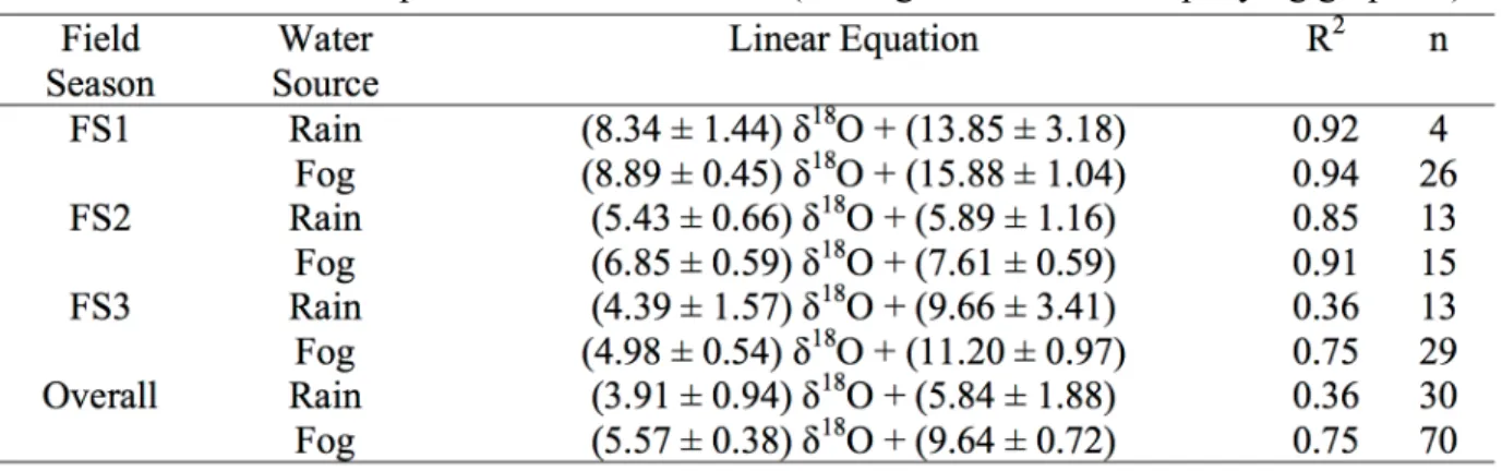
wind speed in daily mean range….……….………...……58 Table V. Linear relationship between δ18O and δ2H (see Figure 12 for
accompanying graphics)……….……..………...…….59 Table VI. Conditions in Galápagos during this study. Precipitation is expressed
as seasonal daily mean and temperature/wind speed in seasonal daily mean
LIST OF FIGURES
Figure 1. Ascension Island location in the South Atlantic Ocean……….28 Figure 2. Daily noontime low cloud base height during the dry season in
Ascension Island, 2015 (METAR, 2015). The dashed line represents the
Height of the peak of Green Mountain, the elevation below which fog can form………..…..…29 Figure 3. Conceptual representation of NDFI, where green reflectance is
lower in cloudier conditions (created with SketchUp software)………...………30 Figure 4. Correlation between DOFmodel and visually classified degree-of-fogginess….……….31
Figure 5. OOB-predicted DOFmodel versus actual DOFmodel, to assess the efficacy
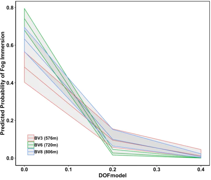
of the random forest model……….………..32 Figure 6. Marginal effects plot for logistic regression validation model………..33 Figure 7. a) Diurnal pattern of DOFmodel with elevation. The diurnal pattern of
DOFmodel was calculated as the average DOFmodel for a given camera over one
foggy season (Aug-Dec 2016) for each half hour at each site. Values were omitted for a given camera/time when <70% of the DOFmodel data was available
due to low lighting conditions (see Methods for details) b) Diurnal pattern of dewpoint depression with elevation, calculated as average dewpoint depression
over one foggy season (Aug-Dec 2016) for each half hour.……….34 Figure 8. Hydroclimatic variation of daily average temperature, RH, and wind
speed and monthly total precipitation during our study period in San Cristóbal Island, Galápagos. Shaded boxes represent FS during which data was collected.
Note that precipitation data is missing prior to ~day 20 of FS1. ……….………60 Figure 9. Field site adjacent to El Junco Lake, San Cristóbal Island. The two
photos at El Junco demonstrate differential fog inundation conditions between FS1 (top) and FS3 (bottom), both dry seasons. This demonstrates the high
interannual variability of fog occurrence in Galápagos……….……...61 Figure 10. Fog versus rain oxygen isotopic ratios. Each point represents
co-collected fog/rain samples………….………..62 Figure 11. Precipitation and D-excess values of precipitation samples at the El
Junco field site, San Cristóbal Island, Galápagos. Each box represents a FS of study (from L to R: FS1, FS2, FS3). The solid line indicates the global average rainfall D-excess and the dashed line indicates the seasonal average fog D-excess.
Figure 12. Linear relationship between δ18O and δD of precipitation samples collected on San Cristóbal Island, Galápagos. Isotopic graphs are separated by FS1 (L), FS2 (middle), FS3 (right), and an overall representation of water isotopic data from all seasons. On each graph, the LMWL is displayed in orange, the GMWL is displayed in black and the fog line is displayed in a dashed line. Each
line represented has an accompanying equation in Table V………...………..64 Figure 13. Daily total precipitation (blue bars) and potential evapotranspiration
(PET, pink lines) for all three field sites (located at 320, 520, and 670 m, respectively). Panels A, B and C represent field seasons one, two and three, respectively. This graphic visually represents plant water supply (blue bars) versus plant water demand (pink lines). Note that meteorological data is
missing from MIR/CA for FS2, so no graphics could be rendered………..……...………..89 Figure 14. FS1 plant xylem and precipitation isotope values. Panels A, B, and C
represent sequential sampling rounds ~2 weeks apart throughout FS1. Invasive plant xylem values (PSGU in every graph) are shown in red and native plant values (BUGR for MIR, ZAFA for CA and MIRO for EJ) are shown in green. Precipitation values are shown in blue: circles indicate fog samples, diamonds indicate rainfall samples and inverted triangles indicate throughfall samples. Soil samples were not collected for FS1. Dashed lines extending from the plant
xylem samples are for visualization purposes only...……90 Figure 15. FS2 soil, plant xylem and precipitation isotope values. Panels A and
B represent sequential sampling rounds ~1 week apart in FS2. Invasive plant xylem values (PSGU in every graph) are shown in red and native plant values (BUGR for MIR, ZAFA for CA and MIRO for EJ) are shown in green. Precipitation values are shown in blue: circles indicate fog samples, diamonds indicate rainfall samples and inverted triangles indicate throughfall samples. Soil samples at increasing depths are displayed in black. Dashed lines extending
from the plant xylem samples are for visualization purposes only………...………….91 Figure 16. FS2 soil, plant xylem and precipitation isotope values. Panels A, B
and C represent sequential sampling rounds ~2 weeks apart in FS3. Invasive plant xylem values (PSGU in every graph) are shown in red and native plant values (MIRO) are shown in green; note that only samples from one field site (EJ) were collected. Precipitation values are shown in blue: circles indicate fog samples, diamonds indicate rainfall samples, inverted triangles indicate throughfall samples, triangles indicate surface water samples (from EJ Lake) and squares represent groundwater samples. Soil samples at increasing depths are displayed in black. Dashed lines extending from the plant xylem samples are
Figure 17. Plant xylem dual-isotope values for all three FS of study. Panels A, B and C represent samples from EJ, CA and MIR, respectively. Hues of pink indicate invasive plants (PSGU at all sites), and hues of green indicate native plants (from top to bottom: MIRO, ZAFA and BUGR). Precipitation values from each FS are shown as blue points and the black dashed line
represents the GMWL………93 Figure 18. Leaf water potential (Ψ) of native (BUGR, ZAFA and MIRO) and
invasive (PSGU) plant stands at MIR (A), CA (B) and EJ (C) during FS3. Sampling rounds took place on 6/12/16, 6/21/16 and 6/24/16, respectively. Red asterisks denote significant differences (p ≤ 0.05) between species at a given site/round (interspecies assessment) and black asterisks denote significant
differences (p ≤ 0.05) within species at a given site/round (intraspecies assessment)…………..94 Supplementary Figure 1. Map of camera trap locations and approximate orientations
along the BV and Dew Pond Paths ascending Green Mountain. Basemap from Quickbird © [2006] DigitalGlobe, Inc. Imagery acquired by Ascension Island
Government (AIG). See Table I for details on each camera……….100 Supplementary Figure 2. Vegetation features and ROIs for each camera (from top
LIST OF ABBREVIATIONS AND SYMBOLS
δ2H Deuterium (Hydrogen-2)
δ18O Oxygen-18
° Degrees (Celsius)
Ψ Leaf water potential
‰ Permil
AIG Ascension Island Government AMF-1 Ascension Island Site
ANCOVA Analysis of covariance
ARM Atmospheric Radiation Measurement Program AVHRR Advanced Very High Resolution Radiometer
B/W Black and white
BUGR Bursera graveolens (ironwood)
BV Breakneck Valley
BV3 Breakneck Valley three (lowest elevation camera) BV6 Breakneck Valley six (mid-elevation camera) BV8 Breakneck Valley eight (highest elevation camera)
CA Cerro Alto
CL Confidence level
cm Centimeters
CSICs Cloud-sensitive image characteristics D-excess Deuterium excess
DNs Digital numbers
DOE Department of Energy
DOFmodel Degree-of-fog model
EJ El Junco
ENSO El Niño-Southern Oscillation EXIF Exchangeable Image Files
FOV Field-of-view
FS1 Field Season One
FS2 Field Season Two
FS3 Field Season Three
GMW Global Meteoric Water Line
GNIP Global Network of Isotopes in Precipitation
GOES Geostationary Operational Environmental Satellite system GOES-R ABI “” Advanced Baseline Imager
ITCZ Intertropical Convergence Zone
KAZRARSCL KA-band ARM Zenith Radars Active Remote Sensing of Clouds Product
LMWL Local meteoric water line LWP Leaf water potential
m/s Meters per second
MAP Mean annual precipitation
MASL Meters above sea level (elevation)
MIR Mirador
mm/hr Millimeters per hour
mL Milliliters
MODIS Moderate Resolution Imaging Spectroradiometer
MPL Micropulse LiDAR
MSG SEVIRI Meteosat Second Generation Spinning Enhanced Visible and Infrared Imager
Myr Million years
NDFI Normalized Difference Fog Index
OOB Out-of-bag
P Total annual precipitation
p-value Statistical significance value PET Potential evapotranspiration PSGU Psidium guajava (guava) R2 Linear correlation coefficient RGB Red-green-blue (color image)
RH Relative humidity (%)
ROI Region of Interest
SE Southeast
SST Sea Surface Temperature std dev Standard deviation TWI Trade wind inversion
CHAPTER ONE: INTRODUCTION
(Held and Soden, 2006; Chadwick et al., 2015). Together, these three issues of water supply, water quality and mounting climate change comprise some of the most predominant global-scale water issues.
Freshwater availability is of particular concern in the tropics, as they are home to some of the most quickly urbanizing regions on the planet (Newman et al., 2006). Despite housing over half of the world’s renewable freshwater resources, almost half of the population is already vulnerable to water stress (James Cook University, 2014). The tropics are dominated by ‘humid tropical’ and ‘arid/semi-arid’ climates, including some of the driest regions in the world (Chen and Chen, 2013). Water-limited environments (where annual precipitation is lower than annual plant water demand) such as these arid/semi-arid regions in the tropics are characterized by low and extremely variable precipitation, sensitivity to environmental change and potential for catastrophic change (Breshears, 2005). Although variable in their geology and vegetation, these regions are particularly susceptible to climate change-related impacts, especially those related to increased freshwater stress (Parry et al., 2008). Examples of hydrologically-related climate change impacts include decreased fog water input (particularly in the dry season) (Johnstone and Dawson, 2010), substantial shifts in regional rainfall patterns (Chadwick et al., 2015), and invasive woody plant encroachment (Caldeira et al., 2015; van Kleunen et al., 2015). When such impacts manifest in tandem, understanding how they interact to determine future freshwater availability is of critical importance.
Such issues related to freshwater availability are particularly pressing in tropical islands. Over half of inhabited tropical islands in one particular study (43 islands total) are already facing some degree of freshwater stress, and this issue is predicted to worsen if climate change
because most freshwater in small islands is held in groundwater reserves, whose resource availability is partially determined by the interactions between island geology, topography, and transport dynamics in the critical zone, or the multi-layered interface between groundwater and the atmosphere. Changes in precipitation seasonality, mean annual precipitation (MAP),
evapotranspiration (plant water demand) and runoff can easily lead to the depletion of these groundwater stores (Ault, 2016).
Fog, or stratus cloud that resides at the earth’s surface, is a key precipitation input in many island ecosystems (Croft, 2003; Bruijnzeel et al., 2005; Gultepe et al., 2007; Scholl et al., 2011; Koracin et al., 2014; Scholl and Murphy, 2014), and has proven to provide much-needed moisture to otherwise dry or seasonally dry ecosystems (Bruijnzeel et al., 2005; Scholl et al., 2011). Current climate change predictions suggest that higher air temperature will lead to an increase in cloud base height, which will move fog cover upward in elevation; this phenomenon has been termed cloud lifting (Pounds et al., 1999). This implies that many ecosystems
decline clearly underline the necessity to better understand fog dynamics as a whole.
CHAPTER TWO: CHARACTERIZING FOG INUNDATION ALONG A TOPOGRAPHIC GRADIENT ON A TROPICAL ISLAND WITH GROUND-BASED
CAMERAS Introduction
Fog deposition is a significant source of water in the overall water budgets of many seasonally dry tropical ecosystems (Cavelier et al., 1996; Rhodes et al., 2006; Liu et al., 2007; Scholl et al., 2007). Further, many plants in these tropical systems and particularly in islands where freshwater is particularly limited, are known to rely on fog as a water source (Goldsmith
et al., 2012; Gotsch et al., 2014a; Fu et al., 2015). One study in Hawaii, for example,
demonstrated the high capacity of shrubs in foggy, windward-exposed sites to intercept cloud water via stemflow (Takahashi et al., 2011). Other studies have suggested that direct uptake of cloud water from the leaf surface or a potential mixture of stemflow and foliar uptake contribute to a plant’s capacity to intercept cloud water (Pryet et al., 2012; Gotsch et al., 2014b). Despite the clear significance of fog in tropical ecosystems, it is often one of the most poorly quantified components of the water balance (Takahashi et al., 2011).
mechanisms, are advection fog, orographic fog and radiation fog. Advection fog occurs when clouds generated over the ocean are transported from the wind to the coast (Bruijnzeel et al., 2005). Orographic fog, a more local phenomenon, occurs when warm, moist air mass is forced upwards by topography, undergoes adiabatic cooling and condenses when cooling is sufficient for the air mass to reach its dew point (Petersen et al., 2015). Radiation fog, the most local-scale of the three fog types, occurs principally via radiative cooling of stratus cloud tops, which can destabilize the boundary layer via turbulent mixing and bring moister air from above to form fog via fluxes of heat and moisture at the earth’s surface (Bruijnzeel et al., 2005; Gultepe et al., 2007). Radiation fog in particular is known to form less frequently over smooth (soil, concrete) than rough terrain (Gultepe et al., 2007), as the fluxes of water from the canopy play a large role in creating fog in many situations (Azevedo and Morgan, 1974; Dawson, 1998).
Satellite remote sensing is one of the principal methods used to understand
spatiotemporal dynamics of fog inundation in a given region (Gultepe et al., 2007; Koracin et al., 2014). Differences in particle size, particle density, height, and texture allow fog to be
Tropical islands are one of the places on earth where identifying diurnal and topographic variability in fog water deposition is crucial. Many tropical islands face particularly acute freshwater stress because of seasonally-variable rainfall patterns that will likely persist or be exacerbated under future climate change (Sobel et al., 2011; Chadwick et al., 2015), extreme precipitation regimes imposed by events such as ENSO (Holding et al., 2016; Permana et al., 2016; Martin et al., 2018) and high moisture demand by plants (Ault, 2016; Karnauskas et al., 2016). It is therefore unsurprising that many tropical island ecosystems are heavily reliant on fog as a water input, with fog contributing up to 75% of the overall water budget in certain tropical regions (See Review by Bruijnzeel et al., 2011).
Examining fog dynamics in smaller regions of interest such as tropical islands requires data with higher spatial and temporal resolution than is possible via most satellite-based fog detection schemes. Thus, alternative methods such as those utilizing ground-based optical cameras, have been developed to track fog (Bendix et al., 2008; Bradley et al., 2010; Schulz et al., 2014, 2016; Wen et al., 2014; Bassiouni and Scholl, 2015). In one study, a black and white (B/W) webcam was placed above the cloud layer in Southern Ecuador and fog was identified via manually defined brightness thresholds in the images (Bendix et al., 2008). A digital elevation model (DEM) was then projected to the view of the camera to identify the contact points between the terrain and cloud surface (cloud top height). This analysis was novel in that it was one of the first to utilize a simple ground-based webcam system to track fog, but it was limited in that it required a lot of manual classification on the part of the user. Another ground-based camera study also used B/W imagery to determine three levels of fogginess based on
not suitable for variable lighting conditions/viewing geometries and required many calculations to account for these differences during the study period. Following the advent of B/W ground-camera methods, the use of RGB (color) ground-cameras for fog detection became more prevalent. Many RGB, ground-based camera methods for fog detection are premised on Koschmeider’s Law (Middleton, 1952), a theory on the apparent luminance of objects observed against background sky. While studies utilizing this theory have been novel in that they can detect fog immersion with a high degree of accuracy, the methods associated with its inclusion in fog detection algorithms are quite complex (Hautiere et al., 2006; Choi et al., 2014).
complex, not completely automated, and doesn’t account for degree-of-fogginess (e.g. light fog versus heavy fog, which is significant in determining ecosystem freshwater availability).
Here, we propose a simpler ground-based fog detection scheme that builds directly upon that of Bassiouni and colleagues ( 2017) to assess patterns of fog in the island ecosystem of Ascension Island, UK. The objectives of this study were 1) to develop a simple and generalizable model to predict degree-of-fogginess at a given elevation 2) to assess how meteorological drivers of fog vary by topographic position; and 3) to evaluate how fog cover varies diurnally during the foggy/dry season. This type of spatiotemporal characterization of fog is necessary to better understand the role of fog across various tropical island ecosystems.
Methods
Study site
This study was conducted on Ascension Island, an isolated peak on the tropical mid-Atlantic ridge, almost equidistant between South America and Africa (-7.94º S, -14.37º W) (Figure 1). Ascension exhibits a steep microclimate zonation over a dense spatial scale (Duffey and Duffey, 1964). Mean annual precipitation (MAP) varies along steep topographic gradients, ranging from < 200 mm in the arid lowlands to ~700 mm in the humid highlands (Ascension, 2015a). Ascension exhibits distinct interannual variability in total annual precipitation, and demonstrates great spatial variability of rainfall brought on by very localized precipitation events. Interestingly, Ascension also boasts the only completely manmade cloud forest in the world (Ashmole and Ashmole, 2000; Wilkinson, 2004).
windward side of the island and up to the highest elevations (~860 MASL) much of the year, but the most dense fog occurs in the dry/foggy season (August – December) (Duffey and Duffey, 1964).
Several local and mesoscale processes lead to the formation of fog on Ascension. The Ascension region in the SE Atlantic is characterized by a consistent deck of stratocumulus clouds, capped by a low-level inversion generated via widespread subsidence (Krishnamurti et al., 1993; Garstang et al., 1996; Moxim and Levy, 2000; Painemal et al., 2015; Brown, 2016). Ascension experiences near-constant SE trade winds below the trade wind inversion (TWI) (Stein et al., 2015; Rolph, 2016) that exhibits little diurnal variation (Brownlow et al., 2016). The strong trade wind inversion prohibits vertical cloud development above the boundary layer and thus ensures generally low rainfall (Rowlands, 2001). These clouds below the boundary layer are maintained via turbulent mixing and longwave cooling at the cloud top, and are largely maintained via moisture supply from the ocean and atmospheric entrainment of dry air
(Bennartz, 2007).
The SE trade winds supply Green Mountain with moisture to sustain the only completely man-made cloud forest in the world (Wilkinson, 2004). This low cloud cover on Ascension plays a significant role in the local hydrologic cycle, and annually averages ~49% daytime cover (Hahn et al., 2003). Historical data suggests that mean low cloud base height is below the peak of Green Mountain (859 MASL) during much of the dry season, indicating that fog water
Seasonal or interannual patterns of cloud cover at an island-wide scale have never been sufficiently established on Ascension Island (Wilson and Jetz, 2016), suggesting high spatial heterogeneity of cloud cover on the island. This uncertainty highlights the necessity to develop a finer temporal method to monitor cloud cover on Ascension under future regimes of climate change where cloud base height could increase (Pounds et al., 1999; Still et al., 1999) and a potential primary source of water for Ascension cloud forest plants could disappear (Ascension, 2015b). Such analysis, while spatially concentrated, could serve to further the knowledge of the role of fog/low clouds in the tropics and subtropics, regions that currently exhibit disagreements within and between climate models, satellite observations and in-situ observations (Trenberth and Fasullo, 2009; Dim et al., 2011; Eastman and Warren, 2013; Dolinar et al., 2015; Norris et al., 2016).
In-situ, camera-based data collection
Daytime images were recorded at three different elevations using Bushnell Trophy Cam™ trail cameras, from the period between September 13th to December 5th 2016. The cameras were installed every ~100 meters in elevation along the windward-exposed Breakneck Valley path (Table 1 & Supplementary Figure 1). Raw RGB images were captured and archived at 30-minute intervals. Exposure time and white point were adjusted for each camera following (Bassiouni et al., 2017) to get maximum contrast for each image. Each camera’s viewing
the actual altitude of fog immersion. While each camera could be slightly rotated when the SD card is replaced every month, we trace fog only over specifically delineated vegetation features in each camera’s respective FOV that remain constant over time (Supplementary Figure 2).
Image preprocessing
To prepare images for analysis, a few steps were taken to pre-process each batch of images. All image processing was performed in R statistical software (RStudio v. 1.1.383). First, the date/time stamps were extracted from each image from EXIF (Exchangable Image File) metadata using the exifr package (Dunnington and Harvey, 2017). Sunrise and sunset times were then computed for each day in the study period using the StreamMetabolism package (Sefick Jr., 2016); all images taken before sunrise and after sunset on each day of the study were discarded and excluded from analysis so as to only include daytime images. Then, all images that were triggered and not set on the timed interval (every 30 minutes) were discarded. Any daytime images that were taken in greyscale mode due to low-lighting conditions were identified via equal DNs in the R, G and B bands and discarded.
The Normalized Difference Fog Index (NDFI) & Degree-of-Fogginess Model (DOFmodel)
To derive the degree-of-fogginess from the images, we developed a spectral measure based on the optical color images. The biophysical basis of the measure is the spectral signature of green vegetation in the visible spectrum, i.e. higher reflectance in the green wavelength and lower reflectance in the red wavelength, as red light is strongly absorbed by green vegetation. In the presence of fog, the contrast in reflectance between green and red light diminishes (Figure 3). Therefore, we propose a spectral index based on the digital values recorded by the camera in the green and red light, the Normalized Difference Fog Index (NDFI) (Equation 1) where:
𝑁𝐷𝐹𝐼 = &'(()*'(+
To quantify the degree-of-fogginess via the NDFI, we followed a number of image processing steps using the Phenopix package (Filippa et al., 2017). First, we took images from each camera and drew a region of interest (ROI) on a specific vegetation feature to exclude areas in the image with less distinctive spectral signature (Supplementary Figure 2). In designating the ROI for each camera, parts of the vegetation that were subject to move with heavy winds or rain and expose background sky, which could lead to an over-estimation of fog immersion, were excluded. We then applied NDFI to each pixel of each ROI in each image using the Phenopix package. For each image, we discarded negative NFDI values (~2% of values that were faulty, as healthy vegetation should never appear more red than green). From this subset of NDFI values, the NDFI median and NDFI standard deviation were then computed for the ROI in each image. We then developed a simple model to relate the degree-of-fogginess (DOFmodel) in each image to
the NDFI median and NDFI standard deviation within the ROI of each image as (Equation 2):
DOFmodel = NDFImedian + NDFIstd dev (2)
where NDFImedian of each ROI was deemed a robust measure of central tendency, as it is resistant
to outlier pixels. Standard deviation was included in the model to account for variation of degree-of-fogginess. DOFmodel is highest under clear conditions and lowest under dense fog conditions. Validation of degree-of-fogginess model (DOFmodel)
DOFmodel was first validated via a visual evaluation of a random subset of images from
BV8. DOFmodel was further validated via the Active Remote Sensing of Clouds Product Using
via micropulse lidar (MPL), cloud base from the ceilometer and information from radiosonde soundings, rain gauge and microwave radiometer measurements to provide a best estimate of the lowest cloud base height (Clothiaux et al., 2000). Observations of lowest cloud base height from this datastream were extracted on the half hour and compared to DOFmodel observations at all three elevations to validate DOFmodel. Cloud-base heights retrieved from KAZRARSCL were used as the standard estimate of the lowest cloud base height. For each of the three cameras in the Breakneck Valley (BV3, BV6, and BV8), a fog immersion binary outcome was created with value 1 if the detected cloud base was less than or equal to the altitude of the camera (576m, 720m, and 806m respectively). Otherwise, fog immersion was set to 0. First, mean DOFmodel values were calculated for both fog-immersed and non-fog immersed conditions to evaluate the efficacy of DOFmodel. Second, a logistic regression model was run and an odds ratio scale utilized to determine if DOFmodel is a suitable method to determine degree-of-fogginess. The predictors in
the logistic regression model were DOFmodel, camera location treated categorically, and the interaction of DOFmodel and camera location. Taken together, these three validation exercises allowed us to determine whether or not it was appropriate to utilize DOFmodel as a direct proxy
for degree-of-fogginess in the random forest model.
Predicting degree-of-fogginess via a random forest model
We extracted in-situ weather data from the DOE ARM AMF1 site, located below the base of the Breakneck Valley path at ~341 MASL (Cook and Sullivan, 2016; Kyrouac and Springston, 2016). Descriptions of the instrumentation deployed at the AMF1 site are described in other studies (Miller and Slingo, 2007; Mather and Voyles, 2013); only a subset of
topography data could be used as predictors of fog occurrence (Kyrouac and Springston, 2016). The weather variables used included temperature, relative humidity, precipitation, wind speed, atmospheric pressure, dew point, surface soil heat flux, dew point depression, radiative fluxes (upwelling/downwelling shortwave/longwave radiation and net radiation), leaf surface wetness and an overall calculated surface energy balance term (Wang and Rossow, 1995; Wang et al., 1999; Guidard and Tzanos, 2007; Obregon et al., 2011; Bassiouni et al., 2017). Dew point depression was calculated following Bassiouni et al. (2017). Other predictive variables included in our random forest model were elevation, time of day and day of year.
While different thresholds of weather variables conducive to fog formation have been established, they often do not translate beyond a single site. For example, the minimum relative humidity threshold used in other models varies across different regions (~87% to 93%) (Wang and Rossow, 1995; Wang et al., 1999; Guidard and Tzanos, 2007). To create a model that
predicts degree-of-fog at a given camera location from elevation, time, and weather variables, we utilized a random forest model in the R package randomForestSRC (Ishwaran and Kogalur, 2017). This oft-used supervised machine learning approach flexibly models nonlinear associations and interactions via merging multiple decision trees for an accurate and stable prediction while avoiding overfitting (Fernández-Delgado et al., 2014). Random forest models also boast the capacity to measure the relative importance of each feature in the prediction.
Assessing the utility of DOFmodel relative to meteorological measurements
To evaluate the utility of DOFmodel as an index of degree-of-fogginess, a logistic
forests (Fernández-Delgado et al., 2014). Models were compared using the C-statistic, also known as the area under receiver operating characteristic (Harrell et al., 1982). The C-statistic ranges from 0.5 if the model does no better than chance to 1 if the model has perfect
classification performance. The Efron-Gong optimism bootstrap was used to obtain unbiased estimates of out-of-sample classification for the logistic regression model (Efron and Gong, 1983). Out-of-bag (OOB) prediction was used to obtain analogous unbiased estimates of out-of-sample classification performance for the random forest classification model.
Understanding spatiotemporal patterns of degree-of-fogginess
In addition to the random forest model, we utilized Pearson’s R to compare DOFmodel and each meteorological variable to characterize elevation-dependent differences in fog formation mechanisms on Ascension. Seasonally averaged diurnal cycles of fog cover on Ascension were assessed graphically.
Results
DOFmodel as a proxy for degree-of-fogginess
We evaluated the relationship between degree-of-fogginess and DOFmodel with 33 randomly selected color photographs. We calculated DOFmodel for the ROI in each photograph and visually estimated the degree-of-fogginess in each ROI. Figure 4 shows the relationship between visually-derived degree-of-fogginess and DOFmodel, which yielded an R2 value of 0.68 and a p-value of 4.6E-9. The strong linear statistical relationship between degree-of-fogginess and DOFmodel support the use of DOFmodel as a proxy for degree-of-fogginess in color
photographs (Figure 4). This strong linear relationship between degree-of-fogginess and
the spatiotemporal variation of degree-of-fogginess with other commonly meteorological variables. Thus, we use DOFmodel as the independent variable in our random forest model. Validating DOFmodel as a model for degree-of-fogginess
Across all cameras, mean DOFmodel value for fog-immersed conditions was lower than
that for clear conditions (x = 0.06 ± 0.03 for fog-immersed and x = 0.09 ± 0.04 for clear conditions). However, the standard deviation was large between photographs within the same binary “fog-immersed” or “clear” categories.
Then, logistic regression was used to validate DOFmodel as a proxy for
degree-of-fogginess. After controlling for site, DOFmodel was found to have a statistically significant
negative association with fog immersion, with lower values of DOFmodel being associated higher
probability of fog immersion (Table 2). All three sites show this pattern of negative association between DOFmodel and fog immersion (Figure 6). Given the strong correlation between DOFmodel
and degree-of-fogginess, we justify the use of DOFmodel as a proxy for degree-of-fogginess in our
random forest model.
Understanding fog cover (DOFmodel) through random forest
Our random forest model, a simple and automated algorithm for predicting fog cover using local meteorological variables, elevation, time of day and time of year explained 54.2% of the variance in all cameras combined with an out-of-bag error rate of 9E-4. OOB error rate is representative of prediction error in a random forest model, as it is ascertained using the 1/3 of the data not used to train the random forest model. In comparing OOB predicted DOFmodel with actual DOFmodel, we found an R2 value of 0.54 and p-value of <2.2E-16 (Figure 5).
longwave irradiance (R = -0.306) and upwelling shortwave irradiance (R = 0.171). These numbers suggest that dewpoint is a strong metric in determining fog occurrence, as has been found in other regions other regions (Obregon et al., 2011; Bassiouni et al., 2017). The strong negative correlation between downwelling longwave irradiance and DOFmodel suggests that the presence of fog (lower DOFmodel) increases downwelling longwave radiation. Other variables were input into the model, but played a lesser role in predicting DOFmodel at a given time point
when all cameras were considered together (see Discussion for assessment of meteorological variables by camera).
Utility of DOFmodel relative to meteorological measurements
The random forest model achieved a C-statistic of 0.97, indicating near perfect
classification. However, this model had 22 local meteorological variables as predictor variables. In contrast, the logistic regression model only included DOFmodel, camera location treated
categorically (i.e. dummy variables for BV6 and BV8), and the interaction of DOFmodel and
camera location. This logistic regression model attained a C-statistic of 0.73. While the logistic regression model did not perform as well as the random forest model, it used a much smaller set of predictors, generated easily interpreted regression coefficients on the odds ratio with
acceptable performance.
Diurnal- and elevation-based assessment of fog cover: relevant meteorological parameters in predicting fog persistence in near-real time
DOFmodel was applied to three sites ranging from 576-806 MASL along the Breakneck
At BV3 (576 m, Supplementary Figure 2), fog cover peaked after sunrise into the late morning, dissipated throughout the afternoon and increased again through the early evening (Figure 7a). BV3 fog cover exhibited a strong negative correlation with dewpoint depression and especially so during midday hours (Table 3). There seemed to be little seasonal variation at BV3, irrespective of time of day (Table 3). During morning/evening hours, there was a strong positive correlation between fog cover and net radiation/downwelling longwave radiation in particular (Table 3). During midday hours, all radiative fluxes, surface soil heat flux, time of day and wetness were all significantly correlated with fog cover (Table 3).
At BV6 (720 m, Supplementary Figure 2), average fog cover was fairly consistent throughout daytime hours but was lowest in early morning and early evening (Figure 7a). BV6
DOFmodel exhibited a very strong negative correlation between dewpoint depression and fog
occurrence across all times of day (Table 3). In the mornings/evenings, DOFmodel was strongly
positively correlated with downwelling longwave radiation, and in the middle of the day
downwelling longwave and shortwave radiation, net radiation, surface soil heat flux and wetness were all significant (Table 3).
At BV8 (806 m, Supplementary Figure 2), degree-of-fogginess was highest in the early morning and evening hours and lowest in the mid to late morning hours (Figure 7a). In both the mornings/evenings and midday hours, time of day was significantly correlated with fog cover. Day of year was also significantly correlated with fog cover, but most so in the
longwave radiation, downwelling shortwave radiation, net radiation, time of day, and wetness/surface soil heat flux (Table 3).
Discussion
Is DOFmodel a suitable proxy for degree-of-fogginess?
The robust correlation between DOFmodel and visually-derived degree-of-fogginess
(Figure 4) serves as a proof-of-concept that DOFmodel derived from the color photographs is a
suitable proxy for degree-of-fogginess. This relationship was further validated via logistic regression, in which there was a strong negative association between DOFmodel and
degree-of-fogginess across all cameras, which is what we would expect given that we designed DOFmodel to
increase as degree-of-fogginess decreases. In tandem, this data suggests that DOFmodel is a simple
and generalizable model suitable for predicting degree-of-fogginess at a given elevation. Thus, we use DOFmodel as a proxy for degree-of-fogginess in our random forest model. We demonstrate
that DOFmodel presents an attractive alternative to prior methods to detect degree-of-fogginess in
regions where meteorological measurements are costly or difficult to obtain.
Our study also demonstrates the efficacy of using a simple random forest model in
predicting degree-of-fogginess. First, the OOB error rate was low and the R2 value of the random forest model was significant (Figure 5). The value of using a random forest model to predict degree-of-fogginess was further validated via the mean DOFmodel values of cloudy versus
be used in tandem with our simple and generalizable index (DOFmodel) to predict
degree-of-fogginess.
Do fog formation mechanisms vary by elevation?
Across all cameras, dewpoint depression was the single strongest predictor of DOFmodel,
which is to be expected given that temperature and relative humidity conditions are known to play a significant role in fog formation (Wang and Rossow, 1995; Wang et al., 1999; Guidard and Tzanos, 2007; Obregon et al., 2011; Bassiouni et al., 2017). However, the other variables predicting degree-of-fogginess in our model varied between cameras (Table 3). This suggests that different meteorological conditions favor fog formation at different elevations.
Over all cameras, the diurnal course of degree-of-fogginess was clearly related to the diurnal course of dewpoint depression, i.e. the difference between air temperature and dewpoint (Figure 6b). It is clear that generally, a higher dewpoint depression during daytime is correlated with reduced fog cover in the dry study season. However, we note that our meteorological data from a single site located below the base of the Breakneck Valley path at ~341 m, so any lags between maximum dewpoint depression and minimum fog cover are likely a direct result of the difference in elevation between sites. Further, we acknowledge that microclimates likely differ between sites of varying elevation and this meteorological data was intended to be used as a general characterization of site conditions. Future studies could investigate using our method on sites with more local meteorological data.
radiation fog forms again before sunset (Whiteman and McKee, 1982), and fog reached a local maximum at BV3 around 17:00 (Figure 7a), supporting the hypothesis that radiation fog was taking place there. Further evidence for radiation fog at this site is that it is located near the base of a valley on Green Mountain – radiation fog is known to form in steep valleys such as this one in particular (Pilie et al., 1975; Bruijnzeel et al., 2005; Liu et al., 2006). In summation, the diurnal pattern exhibited by BV3 suggests that radiation fog was likely a principal mechanism generating/clearing fog at these elevations, as high morning fog cover followed by rapid
clearance with increased solar radiation during the daytime and higher cover in the early evening is characteristic of radiation fog (Obregon et al., 2011).
Fog cover at BV6, located atop a ridge above the valley on the windward side of Green Mountain, exhibited a different diurnal pattern than BV3. At BV6, fog was consistently most dense in the midday hours (Figure 7a). This diurnal pattern of consistent fog cover even in the times of day in which net radiation is particularly high suggests that a possible combination of orographic and advection fog events took place at this elevation (Cereceda et al., 2002; Westbeld
et al., 2009; Lehnert et al., 2018). Further evidence for advection fog formation is the low sea surface temperature in the general region SE of Ascension Island relative to the land surface temperature. Further evidence for orographic fog at this location is the topographic location of the camera on the windward-exposed side of the island. Together, this information preliminarily suggests that a combination of advection and orographic fog was likely the dominant mechanism generating fog at this location.
topographic position, evidence of wind-driven fog in the field, and high volume of fog water input (Schmitt, unpublished data) suggest that orographic and advection fog likely contributed as well. Therefore, we suggest that advection, orographic and radiation fog all contributed to overall fog water input at BV8. Future work should focus on further disentangling fog formation
mechanisms by elevation. Conclusions
In this study, we create a simple and generalizable model (DOFmodel) to predict
degree-of-fogginess from ground-based optical cameras. We suggest that DOFmodel derived from color
photographs is a suitable proxy for degree-of-fogginess, and in doing so develop the first ever non-binary fog classification system using in-situ cameras. We suggest that DOFmodel presents an
attractive alternative to prior methods to detect degree-of-fogginess in regions where
meteorological measurements are costly or difficult to obtain. Our data also suggests that simple models such as random forest and logistic regression can be used to predict degree-of-fogginess with commonly measured meteorological variables. Finally, we suggest that our random forest model that predicts degree-of-fogginess from ground-based cameras and weather variables can be translated to predict degree-of-fogginess in other remote ecosystems.
Tables and Figures
Table I. Cameras used to detect cloud immersion along Breakneck Valley Path, Ascension Island. Camera/Label (in Appendix 1) Location Description Altitude (m)
BV3 In dense pines 576
BV6 Facing valley just below catchment 720
Table II. Parameter estimates and 95% confidence interval on the log odds ratio scale for the logistic regression model estimating fog immersion as a function of DOFmodel and camera site.
Estimate Lower CL Upper CL p-value
Intercept 1.57 1.34 1.81 <2.00e-16
DOFmodel -9.71 -12.37 -7.14 3.06e-13
BV6 2.07 1.65 2.50 <2.00e-16
BV8 1.80 1.40 2.21 <2.00e-16
DOFmodel *
BV6 -11.77 -16.04 -7.54 5.53e-08
DOFmodel *
BV8 -1.83 -5.54 1.91 0.33
Table III. Pearson’s R values of DOFmodel at three different elevations along Breakneck Valley
Path in relation to meteorological parameters for time frames encompassing all daylight hours (7:00 – 18:30), morning/evening hours (7:00 – 9:00 & 17:00 – 18:30) and midday hours (9:30 – 16:30). Insignificant Pearson’s R values (-0.1 to 0.1) are denoted with an asterisk. Observation period took place from Aug-Dec 2016 (dry, foggy season).
DOFmodel
versus: BV3 BV6 BV8
All
daytime Morning/ evening (7:00-9:00 & 17:00-18:30) Midday (9:30 – 16:30) All
daytime Morning/ evening (7:00-9:00 & 17:00-18:30) Midday (9:30 – 16:30) All
daytime Morning/ evening (7:00-9:00 & 17:00-18:30) Midday (9:30 – 16:30) Dewpoint
depression 0.23 0.28 0.32 0.62 0.56 0.75 0.56 0.43 0.61 Downwelling
longwave radiation
-0.15 -0.17 -0.12 -0.43 -0.38 -0.47 -0.30 -0.22 -0.36
Downwelling shortwave radiation
* * 0.18 0.21 * 0.41 0.25 * 0.29
Net radiation * -0.20 0.17 * * 0.39 0.22 -0.12 0.28
Surface soil
heat flux * * -0.27 * * -0.31 * 0.18 -0.14
Day of year * * * * -0.12 * 0.13 0.27 *
Time of day * * 0.26 * -0.15 * -0.128 -0.23 -0.16
Wetness 0.11 * 0.25 0.14 * 0.28 * -0.21 0.14
Figure 5. OOB-predicted DOFmodel versus actual DOFmodel, to assess the efficacy of the
Figure 7. a) Diurnal pattern of DOFmodel with elevation. The diurnal pattern of DOFmodel
was calculated as the average DOFmodel for a given camera over one foggy season (Aug-
Dec 2016) for each half hour at each site. Values were omitted for a given camera/time when <70% of the DOFmodel data was available due to low lighting conditions (see
Methods for details) b) Diurnal pattern of dewpoint depression with elevation, calculated as average dewpoint depression over one foggy season (Aug-Dec 2016) for each half hour.
DO
Fmo
d
e
l
De
w
Po
in
t
De
p
re
s
s
io
n
(
C
°)
Time of Day
BV3 (576 m)
BV6 (720 m)
CHAPTER THREE: THE ROLE OF FOG, OROGRAPHY AND SEASONALITY ON PRECIPITATION IN A SEMI-ARID, TROPICAL ISLAND1
Introduction
The tropics are concurrently one of the fastest urbanizing regions on the planet and home to the most highly concentrated human populations experiencing water scarcity (Newman et al., 2006; Mekonnen and Hoekstra, 2016). Although variable in their geology and vegetation, water-limited environments in the tropics are characterized by low and extremely variable
precipitation, sensitivity to environmental change and vulnerability to catastrophic change (Breshears, 2005; Parry et al., 2008; Chadwick et al., 2015). This variability and unpredictable nature of precipitation can lead to issues related to freshwater availability. For example, Holding et al. (2016) found that over half of inhabited tropical islands are already facing some degree of freshwater stress, and this issue is predicted to worsen if climate change continues along its current course. In fact, many tropical islands are more susceptible to the effects of depleted drinking water stores than they are to sea level rise (Karnauskas et al., 2016). The Galápagos Islands are no exception to the looming threat of water resource depletion; warming of the equatorial Pacific Ocean over the last 150 years (Cobb et al., 2003; Conroy et al., 2009) warrants an increased focus on understanding water resource variability over both event and seasonal timescales.
While rain is a major form of precipitation in the tropics, fog (stratus cloud that resides at
1This chapter previously appeared in the journal Hydrological Processes. The original citation is as follows: Schmitt
the earth’s surface) is another key precipitation input in many island ecosystems (Croft, 2003; Bruijnzeel et al., 2005; Gultepe et al., 2007; Scholl et al., 2011; Koracin et al., 2014; Scholl and Murphy, 2014) and can provide much-needed moisture to otherwise dry or seasonally dry ecosystems (Bruijnzeel et al., 2005; Scholl et al., 2011). Current climate change predictions suggest that higher air temperatures will lead to an increase in cloud base height, which will move fog cover upward in elevation; this phenomenon has been termed ‘cloud lifting’ (Pounds et al., 1999). This implies that many ecosystems worldwide that rely on fog as a water input are threatened by the impending decrease in fog cover and may experience a sudden loss of a critical source of water (Pounds et al., 1999; Still et al., 1999; Hu and Riveros-Iregui, 2016).
Unfortunately, decline in fog cover over the past century has been observed in certain regions, such as coastal California, Eurasia, South America and China (Warren et al., 2007; Johnstone and Dawson, 2010; Williams et al., 2015; Klemm and Lin, 2016); however, absent from these studies are tropical regions, particularly tropical islands. Thus, there remains a need to better understand rain and fog dynamics in these vulnerable ecosystems.
islands such as Hawaii and Puerto Rico (Scholl et al., 2011). It is most often formed under
stronger trade winds and accompanying low-lying atmospheric inversions (Roe, 2005). Radiation fog, on the other hand, is formed when radiational cooling at nighttime reduces the air
temperature to or below its dewpoint (American Meteorological Society, 2012b) and has been found in other tropical regions with surface water bodies (Bruijnzeel et al., 2005). In the tropics, it often takes place in the cool season under low wind conditions (Bruijnzeel et al., 2005). Understanding that these processes can occur individually or simultaneously, and understanding the degree to which each respective fog formation mechanism contributes to the overall water balance of a given island is crucial in understanding freshwater inputs in a given system (Kaseke et al., 2017).
orographically-generated fog (Feild and Dawson, 1998; Scholl et al., 2007). Thus, pivotal to this approach is the ability to separate fog and rain isotopically; in other words, these two moisture inputs must differ sufficiently for any type of mixing model to be used.
In recent decades, climate change has already caused increased seasonality and increased SST in the Galápagos archipelago (Conroy et al., 2009; Wolff, 2010; Liu et al., 2015). Regional models suggest that there is >90% chance of increased rainfall in the region of Galápagos over the 21st Century (IPCC, 2013), but changes in Galápagos may not necessarily reflect regional patterns and critical downscaling is required to better assess potential island-specific changes (Sachs and Ladd, 2010; Liu et al., 2013). Other global models suggest increased precipitation in the tropics, but also posit that the Intertropical Convergence Zone (ITCZ) could migrate
northwards and lead to lower precipitation in the eastern equatorial Pacific (EEP) (Putnam and Broecker, 2017). Thus, future hydrometeorological conditions in Galápagos remain unclear.
In addition to the seasonality imposed by varying degrees of fog water deposition, the Galápagos Islands are also subject to extreme hydrometeorological events such as El Niño due to their distinct location along the equatorial Pacific (Atwood and Sachs, 2014). During canonical El Niño events, the SE trade winds weaken, the thermocline deepens, upwelling declines and the Galápagos experiences anomalously warm SST (Zhang et al., 2014). Higher SSTs lead to
deterioration of the atmospheric inversion layer, triggering convection and precipitation rates 4-7 times higher than average (Trueman and D’Ozouville, 2010; Atwood and Sachs, 2014). La Niña events, on the other hand, lead to anomalously low SST, strengthening of the SE trade winds, and increased subsidence, leading to drastically low precipitation (Trueman and D’Ozouville, 2010). El Niño strength and intensity have doubled in the past three decades (Lee and
et al., 2014). This will likely result in both extreme floods (El Niño) and extreme droughts (La Niña) in the Galápagos region (Power et al., 2013).
To date, there is only one study that has examined the role of seasonal patterns and extreme events the isotopic composition of precipitation in the Galápagos archipelago (Martin et al., 2018). This study found that on one island in the Galápagos archipelago, Santa Cruz Island, precipitation isotopic composition in the highlands was closely linked to precipitation amount on a monthly timescale, but that this effect was much stronger during the wet season. Further, it found that the process of atmospheric convection was a primary driver of precipitation isotopic variability. Here, we examine whether a similar combination of local and regional processes play a role in the isotopic composition of precipitation on the oldest and easternmost island of San Cristóbal, and how the role of different mechanisms vary on event- and seasonally-based scales throughout the progression of the 2016 El Niño. The overall objective of this study was to characterize the hydrometeorological conditions in the highland region of San Cristóbal Island, Galápagos across three distinct seasons: dry season (FS1), wet El Niño season (FS2) (one of the strongest El Niño events on record), and extremely dry season (FS3). Specifically, we addressed the following questions: 1) Does fog isotopic composition vary on event and seasonal
timescales? 2) What drives the seasonal variability of throughfall isotopic composition? 3) Is the amount effect or moisture source region a more dominant control rainfall isotopic composition? and 4) What are the main drivers of local moisture recycling?
Materials and Methods
Characterizing the Galápagos hydroclimate
occurs in two discrete seasons, as tropical Pacific precipitation is largely dictated by variability with both the ENSO and the annual north–south migration of the Intertropical Convergence Zone (ITCZ) (Figure 8) (Nelson and Sachs, 2016). In Galápagos, the hot/wet season takes place from January to May when the ITCZ is at its southernmost position. It is characterized by very localized and irregular convective rain events, and rainfall amount is positively correlated with SST (Trueman and D’Ozouville, 2010). The interplay between the warm climate and the occasional heavy rain events results in high evapotranspiration rates during this season. The cool/dry season takes place from June to December, when the ITCZ is further north. During much of this season, an inversion layer forms, preventing the further rise of moisture-laden air and leading to the formation of frequent fog above approximately 400 meters above sea level (MASL) (Sachs and Ladd, 2010; Trueman and D’Ozouville, 2010).
A typical cool/dry season is characterized by less rain and more fog input into the ecosystem (Pryet et al., 2012; Percy et al., 2016). In Santa Cruz, it has been demonstrated that fog constitutes 26 ± 16% of the incident rainfall at 650 MASL during the dry season (Pryet et al., 2012). To date, this is the only study that has attempted to quantify and understand the
contribution of fog to the water budget in the Galápagos archipelago. However, this study was limited in that it estimated cloud water interception indirectly via a wet canopy water budget method. To overcome the limitation that cloud water interception varies both spatially and by varying canopy architecture, we build on this prior work by collecting fog outside of the canopy and use stable isotopic methods to distinguish fog from rainfall.
island that encompasses ~558 km2. El Junco Lake, our primary study site, lies at ~670 MASL atop a caldera of an extant volcano in the highlands of San Cristóbal. Interestingly, it is the only permanent freshwater body in the archipelago (Zhang et al., 2014). The small catchment
surrounding the lake (0.13 km2) contributes rainwater to this body of water largely in the wet season of each year (Colinvaux, 1972).
Fog collector design
We modified a Juvik-type fog gauge (Juvik and Ekern, 1978) in light of its prior
performance in study sites with similar variable wind shifts to those that take place in Galápagos (Fischer and Still, 2007; Giambelluca et al., 2011; Holwerda et al., 2011). This gauge is often deployed with an adjustable rain ‘hat,’ which reduces contamination of fog samples by rain. We further modified this design by creating a triple-cylinder mesh collection system in lieu of the commonly used double-cylinder mesh, to increase the surface area of the collection system (Fischer and Still, 2007). After extensive testing, we concluded that the triple-cylinder mesh was useful in collecting fog-only samples, as it provided the maximum amount of surface area for fog collection while preventing the apparatus from collecting rain (as this increase in surface area allowed us to lower the rain hat). While our rain hat was deemed effective, we acknowledge that contamination of fog samples by rainfall during high-wind rainy periods may have taken place, but this potential issue was unavoidable.
Precipitation collection
Water samples (fog, rain and throughfall) were collected at El Junco Lake (~670 MASL), located in the very humid zone of San Cristóbal Island, Galápagos (Figure 9). Rain and
These samples were collected over three field seasons (FS) with variable hydroclimatic
conditions between June 2015 and June 2016 (Figure 8). Samples were collected every 3-8 days, based on precipitation amount and frequency. Mineral oil was placed in all collectors to prevent evaporative enrichment of the oxygen and hydrogen isotopes. All water samples were collected in airtight 15 mL amber bottles, sealed using parafilm, and refrigerated prior to analysis to prevent evaporation and water loss.
Climate variables
Local climate information was collected from a weather station installed adjacent to El Junco and logged at 15-minute intervals. Weather station variables used in this analysis include: air temperature/relative humidity (RH) (model CS215, Campbell Scientific Inc., Logan, Utah), precipitation (tipping-bucket rain gauge, Texas Electronics model TE525WS, Campbell Scientific Inc., Logan, Utah), incoming solar radiation (Apogee Instruments, model CS300 Campbell Scientific Inc., Logan, Utah), soil moisture (model CS616, Campbell Scientific Inc., Logan, Utah), and wind speed/wind direction (R.M. Young, model 03002, Campbell Scientific Inc., Logan, Utah). Local SST was collected on neighboring Santa Cruz Island by the Charles Darwin Foundation (Foundation, 2017). Regional ENSO indices computed via the optimum interpolation (OI) SST v2 analysis (Reynolds et al., 2002) were also utilized.
Isotope analysis and isotope theory
At the end of each field campaign, all samples were analyzed for 18O/16O (δ18O) and
2H/1H (δ2H) using laser spectrometry (Picarro L2130-I, Picarro Inc., Santa Clara, CA, USA).