PubMedCentral-PMC5411679.pdf

(1)

March 6, 2017

Practice of Epidemiology

The

“

Dry-Run

”

Analysis: A Method for Evaluating Risk Scores for Confounding

Control

Richard Wyss*, Ben B. Hansen, Alan R. Ellis, Joshua J. Gagne, Rishi J. Desai, Robert J. Glynn,

and Til Stürmer

*Correspondence to Dr. Richard Wyss, Division of Pharmacoepidemiology and Pharmacoeconomics, Department of Medicine, Brigham and Women’s Hospital and Harvard Medical School, Boston, 1620 Tremont Street, Suite 3030, Boston, MA 02120 (e-mail: [email protected]).

Initially submitted August 26, 2015; accepted for publication June 29, 2016.

A propensity score (PS) model’s ability to control confounding can be assessed by evaluating covariate balance across exposure groups after PS adjustment. The optimal strategy for evaluating a disease risk score (DRS) mod-el’s ability to control confounding is less clear. DRS models cannot be evaluated through balance checks within the full population, and they are usually assessed through prediction diagnostics and goodness-of-ﬁt tests. A pro-posed alternative is the“dry-run”analysis, which divides the unexposed population into“pseudo-exposed”and

“pseudo-unexposed”groups so that differences on observed covariates resemble differences between the actual exposed and unexposed populations. With no exposure effect separating the exposed and pseudo-unexposed groups, a DRS model is evaluated by its ability to retrieve an unconfounded null estimate after adjust-ment in this pseudo-population. We used simulations and an empirical example to compare traditional DRS performance metrics with the dry-run validation. In simulations, the dry run often improved assessment of con-founding control, compared with theCstatistic and goodness-of-ﬁt tests. In the empirical example, PS and DRS matching gave similar results and showed good performance in terms of covariate balance (PS matching) and controlling confounding in the dry-run analysis (DRS matching). The dry-run analysis may prove useful in evaluat-ing confoundevaluat-ing control through DRS models.

causal inference; disease risk score; epidemiologic methods; prognostic score; propensity score

Abbreviations: DRS, disease risk score; PS, propensity score.

Summary scores that reduce baseline covariate informa-tion to a single dimension have become increasingly popular to control confounding in nonexperimental studies. The pro-pensity score (PS), deﬁned as the conditional probability of exposure given a set of observed covariates, has been the most widely used summary score (1,2). An alternative to the PS is the prognostic score, often referred to as the dis-ease risk score (DRS). Unlike the PS, which summarizes covariate associations with exposure, the DRS summarizes covariate associations with potential outcomes (3). Both the PS and the DRS control for confounding by acting as balanc-ing scores. Rosenbaum and Rubin (1) showed that, upon conditioning on the PS, covariates are independent of, or bal-anced across, exposure groups. Hansen (3) showed that the

DRS acts as a “prognostic balancing”score in that, condi-tional on the DRS, covariates are independent of the poten-tial outcome under the control condition. Here, we will refer to the control condition as unexposed.

(2)

analysis can potentially allow researchers to compare a larger proportion of the population across exposure groups com-pared with PS analyses (7).

In practice, the PS and DRS are unknown and must be es-timated from the available data. While both the eses-timated PS and DRS are susceptible to model misspecification, the DRS is particularly vulnerable because of the need to ex-trapolate and make additional assumptions whenfitting the risk model (discussed further below) (3). Assessing the va-lidity offitted DRS models could improve the robustness of DRS analyses; however, although a number of studies have discussed and analyzed methods for evaluating PS models (8–14), there remains little discussion of how DRS models should be evaluated when the goal of the DRS is to control for confounding bias.

In this study we used simulations to compare metrics for evaluating DRS models in their ability to control confound-ing. We compared traditional metrics for evaluating risk models with an alternative strategy termed the“dry-run” analy-sis (15). We demonstrate the discussed concepts through an empirical example comparing dabigatran with warfarin for preventing ischemic stroke and all-cause mortality within a population of Medicare beneﬁciaries.

METHODS

Modeling the DRS

The DRS has typically been estimated either byfitting a regression model within the unexposed population and then extrapolating this model to predict disease risk for the full cohort or byfitting a regression model within the full cohort as a function of baseline covariates and exposure and then assigning risk scores after setting exposure status to zero (16–22). Hansen (3) discussed limitations to these strategies, both of which are examples of“same-sample”estimation. If the exposure effect is misspecified when fitting the risk model to the full cohort (e.g., omitting exposure-covariate interactions), then the estimated scores can carry informa-tion about the exposure effect. This nonancillarity in the es-timated risk scores can potentially bias effect estimates and generate spurious suggestions of effect modification across levels of disease risk (3,20). Fitting the DRS only to the un-exposed population, however, can lead to overfitting, which can itself cause apparent effect modification and bias overall in effect estimates (3,23,24).

To avoid these problems, both Hansen (3) and Glynn et al. (23) have proposed using a historical set of unexposed subjects toﬁt the DRS model. This strategy can circumvent the problems associated with“same-sample”estimation, but it assumes that the effects of risk factors on the outcome, disease surveillance, and covariate deﬁnitions do not change over time. Violation of these assumptions could result in an estimated DRS model that is not generalizable to the study cohort (7,25,26).

These challenges in estimating the DRS highlight the im-portance of evaluating the validity ofﬁtted DRS models as a way to control confounding. While a PS model’s ability to control confounding can be evaluated directly by assessing covariate balance across exposure groups after PS adjustment,

the prognostic balance resulting from a DRS model can be evaluated only among unexposed individuals, where the po-tential outcome under the unexposed condition is observed. Evaluating prognostic balance among only the unexposed can reward models that are overfitted to the unexposed group and does not necessarily indicate how well prognostic balance is achieved within the entire study population (3, 24). Conse-quently,fitted DRS models have been assessed primarily by using prediction diagnostics and goodness-of-fit tests rather than measures of prognostic balance.

The“dry-run”analysis

Hansen (15) proposed an alternative strategy for evaluating risk scores in their ability to control confounding. Because modeling the PS does not share the same theoretical challenges as modeling the DRS, Hansen (15) explained that researchers can use the estimated PS to divide the unexposed population into“pseudo-exposed”and“pseudo-unexposed”groups in or-der to create differences on observed covariates that are similar to differences between the actual exposed and unexposed populations. With no exposure effect separating the pseudo-exposed and pseudo-unpseudo-exposed groups, analysts can perform a dry-run analysis by ﬁtting the DRS model to the pseudo-unexposed group, or a historical set of pseudo-unexposed subjects, and then evaluating the validity of the risk score setup by its ability to control confounding within the pseudo-population. If subclassiﬁcation or matching on the estimated DRS results in unconfounded null effect estimates within the pseudo-population, then the modeling procedure should be successful in controlling confounding on the same observed covariates when applied to the original sample. We describe the dry-run analysis in detail below and provide example code in Web Appendix 1 (available athttp://aje.oxfordjournals.org/):

1. Estimate the PS within the full study population. This step entails diagnosing the PS model’s validity (e.g., checking positivity violations, calibration, discrimin-ation, covariate balance, etc.).

2. Create a pseudo-exposure group by sampling, without re-placement, a subset of unexposed subjects with sampling probabilities arranged so that the odds of selection for pseudo-exposure are proportional to the odds of the esti-mated PSs from step 1. Sampling should be done so that the proportion of the pseudo-exposed within the full un-exposed population is approximately equal to the propor-tion of the exposed within the full study populapropor-tion. Here, we describe a simple procedure that uses indepen-dent Bernoulli sampling to select the pseudo-exposure group. Other sampling procedures could also be em-ployed (see Web Appendix 1).

Letπ = ( + θ )

[ + ( + θ )]

i

c c exp 1 exp

i

i whereθ =i log[( − )] PS

PS 1

i i , and

c

is a constant such that∑₌ π = [ ]

+ n

i n

i n n n u 1

u e

u e (i=1, . . . nu,

(3)

sampling results in an expected size of⎡_⎣ ⎤_⎦

+ n

n n n u

e

u e sub-jects for the pseudo-exposure group but will vary around this target from sample to sample.

3. Form a pseudo-unexposed group consisting of all indivi-duals in the unexposed population who are not sampled into the pseudo-exposure group.

4. Model the DRS within the pseudo-unexposed group or an external set of unexposed subjects.

5. Estimate the pseudo-exposure effect after stratifying or matching on the estimated DRSs within the pseudo-population, and calculate the pseudo-bias, deﬁned as the difference between the pseudo-effect estimate and the true null effect.

6. Bootstrap (i.e., repeat) steps 2–5 to form a distribution of calculated pseudo-biases whose mean and corresponding conﬁdence limits can be used to evaluate the validity of theﬁtted DRS model.

The sampling outlined above results in a pseudo-population in which the odds of selection for pseudo-exposure are pro-portional to the estimated odds of exposure in the full popu-lation. The goal of the dry-run sampling is not to create pseudo-exposed and pseudo-unexposed groups where co-variate distributions mirror those of the full exposed and un-exposed populations, but rather it is to create differences between the pseudo-exposed and pseudo-unexposed groups that are similar to observed differences in the full population. For example, suppose we have a cohort where the average age among the exposed is 50 years, the average age among the unexposed is 40 years, and there are equal numbers of exposed and unexposed. The goal of the dry-run sampling is to create pseudo-exposed and pseudo-unexposed groups that differ by 10 years on average, matching the difference be-tween the exposed and unexposed. That could happen with a mean age of 45 years within the pseudo-exposed and 35 years within the pseudo-unexposed, resulting in a difference of 10 years while maintaining the overall average of 40 years across unexposed subjects.

Therefore, prior to mounting a full dry-run validation, analysts should check that differences in baseline character-istics between the pseudo-exposed and pseudo-unexposed groups resemble differences between the actual exposed and unexposed populations. If the PS model is well-speciﬁed, while positivity assumptions hold also, there should be such a similarity. It will of course be inexact; one is looking for gross departures here.

Simulation study

We simulated a dichotomous exposure (A) and outcome (Y), 6 binary covariates (X1, X3, X5, X6, X8, X10) and 4

standard-normal covariates (X2, X4, X7, X9). We deﬁned

the conditional probability of exposure and outcome accord-ing to equations1and2.

( [ | ]) = α + α + ⋯ + α + α

+ α + α + α + α ( )

E A X X X X X

X X X X X X

logit

. 1

i 0 1 1 10 10 11 2 3 12 4 8 13 5 6 14 72 15 102

( [ | ]) = β + β + ⋯ + β

+ β + β + β

+ β + β + β ( )

E Y X A X X

X X X X X X

X X A

logit ,

. 2

i

A

0 1 1 10 10

11 2 3 12 4 8 13 5 6

14 72 15 102

The coefficient values forαi andβi,i=1 . . . 15, were se-lected by drawing values from separate uniform(−0.7, 0.7) distributions. This range of values (i.e., potentially ranging from−0.7 to 0.7) was chosen to reflect the range for the ma-jority of coefficient values observed in an empirical example comparing dabigatran with warfarin that is described in the next section. We repeated this process 100 times by drawing a separate set of values forαiandβi,i=1 . . . 15, to consider a total of 100 unique parameter combinations. To avoid is-sues with the collapsibility of the odds ratio, we held the ex-posure effect constant at an odds ratio of 1 (i.e., β =_A 0) (27). Bothα0andβ0were set so that the baseline prevalence

of exposure and baseline incidence of the outcome were 30% (i.e., baseline prevalence and incidence when all co-variate values are set to 0).

With each parameter combination we simulated a study cohort and a historical set of unexposed subjects that was similar to the study cohort but with no exposure in-troduced. Weﬁtted 32 unique DRS models within this his-torical population using logistic regression with various degrees of model misspeciﬁcation. Each of the models included main effects for the covariatesX1throughX10but

different sets of higher-order terms. We considered all possible combinations of the higher-order terms shown in equation2(32 in total). We evaluated the calibration and discrimination for each DRS model by calculating the Hosmer-Lemeshow Pvalue andCstatistic within the ori-ginal cohort. We also evaluated each DRS model by con-ducting a dry-run validation as described previously. Because the dry-run analysis relies on using the PS to cre-ate the sampling probabilities, we estimcre-ated the PS using 4 different logistic models with varying degrees of misspeciﬁ ca-tion: PS model 1 (included all higher-order terms), PS model 2 (excluded 1 interaction term), PS model 3 (excluded 1 interaction term and 1 quadratic term), and PS model 4 (excluded all higher-order terms).

We conducted simulations using sample sizes of 10,000, 5,000, and 2,000. We estimated the exposure effect within the original study population and each of the pseudo-populations after stratifying on quintiles of the estimated DRS and after matching on the estimated DRS. One-to-one caliper match-ing was done without replacement usmatch-ing a caliper width of 0.2 standard deviations of the respective DRS distribution (28,29).

(4)

Empirical example

We compared the performance of dabigatran versus war-farin in a nonselected population of older US adults using a 20% random sample (n= 67,667) of all patients with fee-for-service Medicare parts A (hospital), B (outpatient), and D (pharmacy) coverage for at least 1 month from October 19, 2010, through December 31, 2012. Details of the study population and cohort creation are provided elsewhere (7).

We modeled the 1-year risk of combined ischemic stroke and all-cause mortality within a historical population of new warfarin users (30) with an index date prior to the introduction of dabigatran (from January 1, 2008, through October 18, 2010). This model was then used to predict the disease risk for all individuals within the study cohort. Weﬁtted PS and DRS

models that included main effects for 37 a priori selected cov-ariates and an additional 200 empirically selected covcov-ariates that were identified within Medicarefiles containing medica-tion claims, inpatient and outpatient diagnostic codes, and pro-cedural codes. The estimated scores were implemented using 1-to-1 matching without replacement. Details of covariate se-lection and definitions are provided elsewhere (7).

To evaluate the validity of theﬁtted DRS model, we cre-ated a pseudo-exposure group by sampling new warfarin users within the original study cohort (i.e., index date after October 18, 2010), using the sampling described previously. We created a pseudo-unexposed group consisting of new warfarin users who were not selected into the pseudo-exposure group. We then evaluated the validity of the histor-icallyﬁtted DRS model by observing how well matching on

abs.Pseudo1 abs.Pseudo2 abs.Pseudo3 abs.Pseudo4 C Statistic P Value 0.0

0.2 0.4 0.6 0.8 1.0

Evaluation Metric

Correlation Coefficient Squared

A)

Pseudo1 Pseudo2 Pseudo3 Pseudo4 C Statistic P Value

0.0 0.2 0.4 0.6 0.8 1.0

Evaluation Metric

B)

0.2 0.4 0.6 0.8 1.0

Evaluation Metric

C)

0.0 0.2 0.4 0.6 0.8 1.0

Evaluation Metric

D)

0.2 0.4 0.6 0.8 1.0

Evaluation Metric

E)

0.0 0.2 0.4 0.6 0.8 1.0

Evaluation Metric

F)

(5)

the estimated scores controlled for confounding within the pseudo-population. We bootstrapped this process 1,000 times and took the mean of the pseudo-bias across all boot-strapped runs as the measure for modelﬁt. For comparison, we also evaluated the performance of the estimated DRSs by assessing the calibration (Hosmer-Lemeshow goodness-of-ﬁt test) and discrimination (C statistic) of the predicted values within the original study cohort.

RESULTS

Simulation results

Figures1and2show box plots for the Spearman correla-tion coefﬁcients between each of the described measures

and both the absolute bias (Figure1A,1C, and1E) and bias (Figure 1B, 1D, and 1F) in the estimated exposure effect. The absolute pseudo-bias was used when comparing mea-sures with the absolute bias. In Figure 1, exposure effects were estimated through DRS stratiﬁcation, while in Figure2 the exposure effects were estimated through DRS matching. Each box plot shows the distribution of 100 correlation

coef-ﬁcients (1 correlation coefﬁcient for each of the 100 para-meter combinations).

When the estimated PS was a close approximation to the true PS model (PS models 1 and 2), there was a strong cor-relation between the pseudo-bias and the actual bias within the original study cohort (Figures1and2). As the

misspeci-ﬁcation in the PS model increased, the strength of this cor-relation became less pronounced and theCstatistic showed

0.2 0.4 0.6 0.8 1.0

Evaluation Metric

A)

0.0 0.2 0.4 0.6 0.8 1.0

Evaluation Metric

B)

0.2 0.4 0.6 0.8 1.0

Evaluation Metric

C)

0.0 0.2 0.4 0.6 0.8 1.0

Evaluation Metric

D)

0.2 0.4 0.6 0.8 1.0

Evaluation Metric

E)

0.0 0.2 0.4 0.6 0.8 1.0

Evaluation Metric

F)

(6)

a stronger correlation in predicting bias (Figures1and2). Compared with DRS stratiﬁcation, matching on the esti-mated DRSs resulted in a weaker correlation between the pseudo-bias and actual bias in the effect estimate (Figures1 and2). The pseudo-bias showed a stronger correlation with bias in the effect estimate compared with the correlation be-tween the absolute pseudo-bias and absolute bias in the effect estimate (Figures1and2). As the sample size decreased, the correlation between the pseudo-bias and bias in the effect es-timate was attenuated, but the pseudo-bias was still generally stronger in predicting bias compared with theCstatistic and Hosmer-LemeshowPvalue.

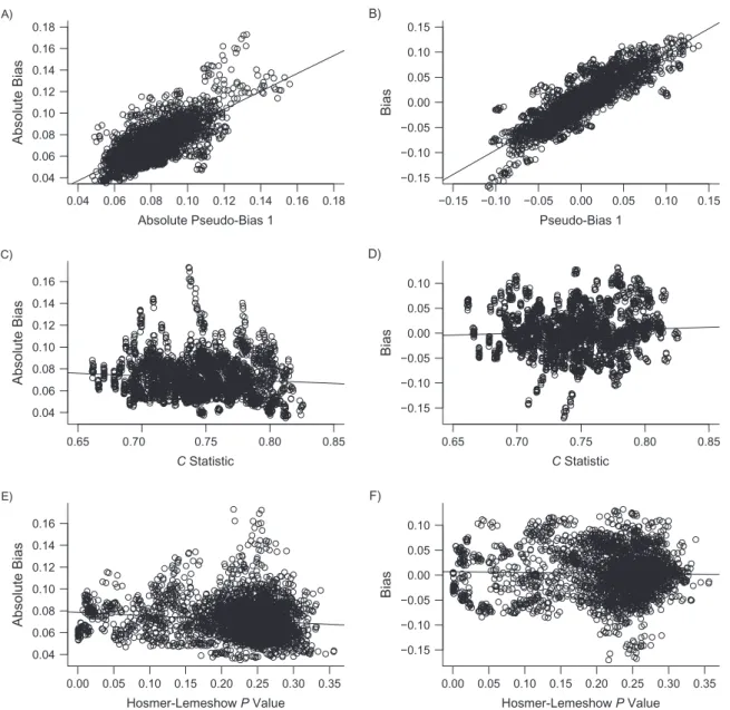
Figure3shows each measure plotted against the absolute bias (Figure3A,3C, and3E) and bias (Figure3B,3D, and3F) in the effect estimate after combining the values for each meas-ure across all parameter combinations and models. For ex-ample, for Figure3A and3B we calculated 3,200 pseudo-bias measures (32 DRS models × 100 parameter combinations) when using PS model 1 to create the pseudo-populations. Figure3A and3B plot the absolute pseudo-bias (Figure3A) and pseudo-bias (Figure 3B) under PS model 1 against the corresponding absolute bias (Figure3A) and bias (Figure3B) in the exposure effect estimate from the original study cohorts. Similar descriptions can be applied to Figure3C and3D for

0.04 0.06 0.08 0.10 0.12 0.14 0.16 0.18 0.04

0.06 0.08 0.10 0.12 0.14 0.16 0.18

Absolute Pseudo-Bias 1

Absolute Bias

A)

−0.15 −0.10 −0.05 0.00 0.05 0.10 0.15

Pseudo-Bias 1

Bias

B)

0.65 0.70 0.75 0.80 0.85

0.04 0.06 0.08 0.10 0.12 0.14 0.16

C Statistic

Absolute Bias

C)

0.65 0.70 0.75 0.80 0.85

−0.15 −0.10 −0.05 0.00 0.05 0.10

C Statistic

Bias

D)

0.00 0.05 0.10 0.15 0.20 0.25 0.30 0.35 0.04

0.06 0.08 0.10 0.12 0.14 0.16

Hosmer-Lemeshow P Value

Absolute Bias

E)

0.00 0.05 0.10 0.15 0.20 0.25 0.30 0.35 −0.15

−0.10 −0.05 0.00 0.05 0.10

Hosmer-Lemeshow P Value

Bias

F)

(7)

theCstatistic and Figure3E and3F for the Hosmer-Lemeshow Pvalue. Similar to Figures1and2, when the estimated PS was correctly speciﬁed, the pseudo-bias showed the strongest corre-lation with bias and had an intercept from the least-squares regression line of approximately 0 (Figure3A and3B). Both theCstatistic and thePvalue from the Hosmer-Lemeshow test showed weaker correlations after combining results across dif-ferent data-generating models (Figure3C–3F).

Figures1and2show that the value of the dry-run pseudo-bias as an indication for pseudo-bias in the full study cohort is affected by the specification of the PS model and sample size. To examine other factors that may influence the per-formance of the dry-run analysis in more detail, we con-ducted a number of sensitivity analyses where we varied the prevalence of exposure, the degree of separation in the PS distributions, the correlation between the PS and DRS, and the exposure effect. A detailed description of these additional simulations is provided in Web Appendix 2. Results showed that the prevalence of exposure, separation in PS distribu-tions, and correlation between the PS and DRS can also influence the performance of the dry-run analysis. When the PS was correctly specified, however, the pseudo-bias gener-ally performed well in predicting bias in the effect estimate compared with theCstatistic and Hosmer-LemeshowPvalue (Web Figures 1–8).

Empirical results

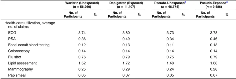
We present results for the empirical study in Figure4and Tables1and2. Figure4shows good overlap in PS distribu-tions across the dabigatran (exposed) and warfarin (unexposed) exposure groups. Table1shows the distribution of 37 a priori selected covariates across exposure groups and across the sampled pseudo-exposed and pseudo-unexposed groups (co-variate values for the pseudo-population were averaged over all bootstrapped runs). New users of dabigatran were generally healthier with fewer comorbidities than new users of warfarin (Table1) (31,32). In general, differences between the pseudo-exposed and pseudo-unpseudo-exposed groups paralleled differences between the dabigatran and warfarin groups (Table1).

Table2shows that both PS and DRS matching resulted in similar effect estimates, with hazard ratios of 0.88 (95%

con-fidence interval: 0.81, 0.95) and 0.87 (95% confidence inter-val: 0.81, 0.94), respectively. Thefitted PS model resulted in good predictive performance and model fit in terms of dis-crimination and calibration, with a C statistic of 0.73 and Hosmer-Lemeshow P value of 0.18 (Table 2). The fitted DRS also resulted in good discrimination, with aCstatistic of 0.78, but poor calibration in terms of the Hosmer-Lemeshow goodness-of-fit test, with aPvalue of<0.01 (Table2). After matching on the PS, exposure groups were approximately ba-lanced on measured covariates with an average standardized absolute mean difference of<0.01. Matching on the DRS re-sulted in a pseudo-bias of approximately−0.02 (95% confi -dence interval:−0.1, 0.06) (Table2).

DISCUSSION

In this study, we used simulations and an empirical ex-ample to compare metrics for evaluating DRS models in their ability to reduce bias in effect estimates. We considered 2 traditional measures of model performance: the C statistic and thePvalue from the Hosmer-Lemeshow goodness-of-ﬁt test. We also considered the dry-run method proposed by Hansen where the PS is used to divide the unexposed popu-lation into pseudo-exposed and pseudo-unexposed groups, and theﬁtted DRS is then evaluated by its ability to control for confounding within this pseudo-population (15).

In simulations, the pseudo-bias from the dry run had the strongest correlation with bias in the effect estimate when the functional form of the PS was a close approximation to the true PS model. When there was moderate to severe misspecifi ca-tion in the PS, this correlaca-tion was attenuated and theC statis-tic showed a stronger correlation with bias in these settings. The Cstatistic performed well when comparing the relative performance of different modelsfitted to the same data set. In practice, however, researchers will often fit a single model and want to assess its validity in terms of confounding control. In simulations, the C statistic showed little correlation with bias after combining results across all simulation scenarios,

0.0 0.2 0.4 0.6 0.8 1.0

0 1 2 3 4

Propensity Score Distribution

Density

A)

0.0 0.2 0.4 0.6 0.8 1.0

0 1 2 3 4

Propensity Score Distribution

Density

B)

(8)

Table 1. Baseline Covariates Across Dabigatran and Warfarin Exposure Groups and Pseudo-Exposed and Pseudo-Unexposed Groups in a Population of Medicare Beneﬁciaries, United States, 2010–2012

Warfarin (Unexposed) (n=56,260)

Dabigatran (Exposed) (n=11,407)

Pseudo-Unexposeda

(n=46,774)

Pseudo-Exposeda

(n=9,486)

No. of

Participants %

No. of

Participants %

No. of

Participants %

No. of

Participants %

Demographics

Mean age, years 78.9 76.8 79.3 77.1

White, % 50,185 89.2 10,462 91.7 41,514 88.8 8,671 91.4

Female sex, % 23,726 42.2 5,584 49.0 19,206 41.1 4,520 47.6

Diagnoses Cardiovascular

Chest pain 21,608 38.4 3,998 35.0 18,270 39.1 3,338 35.2

Heart disease 41,945 74.6 7,599 66.6 35,535 76.0 6,410 67.6

Heart failure 17,297 30.7 2,194 19.2 15,291 32.7 2,006 21.1

Hypertension 36,616 65.1 7,221 63.3 30,598 65.4 6,018 63.4

Hyperlipidemia 19,807 35.2 4,687 41.1 16,032 34.3 3,775 39.8

Myocardial infarction 1,965 3.5 216 1.9 1,764 3.8 201 2.1

Cerebrovascular disease 11,979 21.3 1,982 17.4 10,253 21.9 1,726 18.2

Stroke

Ischemic 3,427 6.1 492 4.3 2,976 6.4 451 4.8

Hemorrhagic 189 0.3 18 0.2 173 0.4 16 0.2

TIA 3,882 6.9 723 6.3 3,264 7.0 618 6.5

VTE 5,829 10.4 191 1.7 5,627 12.0 202 2.1

Diabetes 19,744 35.1 3,424 30.0 16,801 35.9 2,943 31.0

Kidney disease 7,076 12.6 541 4.7 6,553 14.0 523 5.5

Renal failure 9,053 16.1 656 5.8 8,410 18.0 643 6.8

Bleeding 1,058 1.9 78 0.7 982 2.1 76 0.8

Anemia 8,792 15.6 1,135 10.0 7,788 16.6 1,004 10.6

Baseline medications

Antidepressant 15,902 28.3 2,611 22.9 13,664 29.2 2,238 23.6

Antihypertensive

ACE/ARB 29,377 52.2 5,730 50.2 24,567 52.5 4,810 50.7

Loop diuretic 23,018 40.9 3,274 28.7 20,075 42.9 2,943 31.0

Nonloop diuretic 29,565 52.6 4,788 42.0 25,379 54.3 4,186 44.1

Hypolipidemic

Statin 27,795 49.4 5,983 52.5 22,884 48.9 4,911 51.8

Fibrate 2,827 5.0 568 5.0 2,353 5.0 474 5.0

Rate control therapy

Beta blocker 39,850 70.8 8,212 72.0 33,062 70.7 6,788 71.6

CCB 24,739 44.0 4,768 41.8 20,730 44.3 4,009 42.3

Glycoside 10,401 18.5 1,951 17.1 8,734 18.7 1,667 17.6

Rhythm control therapy 10,745 19.1 2,648 23.2 8,684 18.6 2,061 21.7

(9)

illustrating that the actual value of aCstatistic does not pro-vide the best information for testing the validity of a singleﬁ t-ted DRS model.

While the dry-run validation can assess whether a fitted DRS model is insufficient in terms of confounding control, it does not provide information on whether the lack of con-founding control is due to model misspecification or model extrapolation. Extrapolation being done by the risk score, however, can potentially be mitigated by the process offitting and checking the validity of the PS (e.g., identifying positivity violations). Although the presence of a few high-propensity unexposed subjects could lead to especially problematic extrapolation, this situation would reduce the pseudo-variance relative to the pseudo-bias, increasing the likelihood of reject-ing the risk score setup. In other words, the dry-run validation penalizes a risk score for extrapolation.

A few limitations of the dry-run validation deserve atten-tion. Because the dry run uses the PS to create sampling

probabilities, the method’s application is constrained by the assumptions of the PS, even though analyses using the DRS do not inherit these stronger assumptions. In particular, the PS requires that there be no covariate patterns at which exposure is received with certainty (i.e., positivity) (33). The DRS re-quires a weaker condition, that there be no levels of disease risk at which exposure is certain (i.e., risk positivity) (3). While analyses using the DRS may include some individuals for whom positivity is violated, the dry run’s application is limited to the population where positivity holds. If the analyst determines that positivity is violated when assessing the appro-priateness of theﬁtted PS model, then the analyst must decide whether to respecify the PS and try again, restrict the analysis to a subgroup for which positivity does appear to hold, or seek other modes of validation for the risk score model.

The dry-run analysis also requires accurate estimation of the PS. In this case, one could simply use the PS for confounding control. The DRS, however, can be valuable even when a Table 1. Continued

Warfarin (Unexposed) (n=56,260)

Dabigatran (Exposed) (n=11,407)

Pseudo-Unexposeda

(n=46,774)

Pseudo-Exposeda

(n=9,486)

No. of

Participants %

No. of

Participants %

No. of

Participants %

No. of

Participants %

Health-care utilization, average no. of claims

ECG 3.74 3.80 3.73 3.78

PSA 0.36 0.49 0.34 0.46

Fecal occult blood testing 0.12 0.13 0.11 0.13

Colonoscopy 0.14 0.14 0.14 0.14

Flu shot 0.76 0.79 0.75 0.79

Lipid assessment 1.52 1.72 1.48 1.68

Mammography 0.25 0.29 0.24 0.28

Pap smear 0.05 0.07 0.05 0.07

Abbreviations: ACE/ARB, angiotensin-converting enzyme/angiotensin II receptor blocker; CCB, calcium channel blockers; ECG, electrocardio-graphy; PSA, prostate-speciﬁc antigen; TIA, transient ischemic attack; VTE, venous thromboembolism.

a_{Mean values for each covariate averaged over 1,000 sampled pseudo-populations. The total}_n_{and numbers of each covariate in the} pseudo-exposed and pseudo-unpseudo-exposed groups were rounded to the nearest whole number.

Table 2. A Comparison of Effect Estimates on the Basis of Propensity Score or Disease Risk Score Matching in New Users of Dabigatran and Warfarin in a Population of Medicare Beneﬁciaries (n=67,667), United States, 2010–2012

Methoda HR 95% CI Pseudo-Biasb 95% CI ASAMDc CStatistic HLPValued

Unadjusted 0.48 0.46, 0.50 −0.57 −0.65,−0.50 0.14

PS matching 0.88 0.81, 0.95 <0.01 0.73 0.18

DRS matching 0.87 0.81, 0.94 −0.02 −0.10, 0.06 0.78 <0.01

Abbreviations: ASAMD, average standardized absolute mean difference; CI, conﬁdence interval; DRS, disease risk score; HL, Hosmer-Lemeshow; HR, hazard ratio; PS, propensity score.

a_{PS and DRS models included 200 empirically selected covariates and 37 covariates selected a priori.}

b_{Bias in the pseudo}_–_{effect estimate on the log scale (averaged across 1,000 bootstrapped samples). The unadjusted pseudo-bias was} calcu-lated by taking the log of the unadjusted hazard ratio within the pseudo-population. The DRS-matched pseudo-bias was calcucalcu-lated by taking the log of the hazard ratio obtained after matching pseudo-exposed to pseudo-unexposed subjects.

c_{ASAMD of covariates across exposure groups.}

(10)

correctly specified PS is available. As discussed in the Intro-duction, risk scores are often preferred for evaluating effect measure modification. The use of risk scores for evaluating ef-fect modification, however, is challenging because misspecified or overfitted DRS models can produce spurious suggestions of effect modification across levels of disease risk (3,15,34). In theory, the dry-run validation could be used to detect false sig-nals of effect modification (15). If the modeling procedure pro-duces risk scores that result in the appearance of effect modification within the pseudo-population, this would bring into question the value of the risk score setup for evaluating ef-fect modification when applied to the full study population.

With a correctly speciﬁed PS, one may wish to evaluate a DRS model by comparing results from DRS and PS analy-ses. The dry-run strategy, however, maintains objectivity in study design (35). By restricting to the unexposed popula-tion when evaluating risk models, the dry-run analysis does not allow information about the exposure-outcome associ-ation to contribute to decisions on model selection. Re-searchers can evaluate and modifyﬁtted risk models within the sampled pseudo-population without the risk of degrad-ing inference (3,15).

Finally, the optimal strategy for sampling from the unex-posed population when performing a dry-run analysis remains unclear. The without-replacement sampling outlined in this study performed well for the scenarios considered. For smaller samples, other without-replacement sampling techniques may be more appropriate. These could include maximum entropy sampling, which allows the analyst to explicitly specify the number to be sampled (36), or a rejection sampling scheme that throws out a particular pseudo-exposure group selection if its size falls outside of a predetermined window. Regardless of the sampling technique used, we emphasize that the dry-run analysis does not provide information about bias caused by unmeasured confounding. Subject-matter expertise is a necessary component when performing PS or DRS analyses (37,38).

We conclude that accurately modeling the DRS within the study cohort or within a historical set of unexposed sub-jects presents unique challenges that are not shared by the PS. Measures of predictive performance and goodness-of-ﬁt tests do not necessarily describe the ability of a DRS model to control confounding. If the PS can be accurately modeled, evaluating the ability of the DRS model to control con-founding within a dry-run analysis can provide insight into the validity ofﬁtted DRS models.

ACKNOWLEDGMENTS

Author afﬁliations: Department of Epidemiology, Gillings School of Global Public Health, University of North Carolina, Chapel Hill, North Carolina (Richard Wyss, Til Stürmer); Division of Pharmacoepidemiology and Pharmacoeconomics, Department of Medicine, Brigham and Women’s Hospital and Harvard Medical School, Boston, Massachusetts (Richard Wyss, Joshua J. Gagne, Rishi J. Desai, Robert J. Glynn); Department of Statistics, College of Literature, Science, and the Arts, University of

Michigan, Ann Arbor, Michigan (Ben B. Hansen); and Department of Social Work, College of Humanities and Social Sciences, North Carolina State University, Raleigh, North Carolina (Alan R. Ellis).

This work was funded by the National Institute on Aging (grant R01 AG023178). The database infrastructure used for this project was funded by the Pharmacoepidemiology Gillings Innovation Lab (PEGIL) for the Population-Based Evaluation of Drug Beneﬁts and Harms in Older US Adults (grant GIL200811.0010); the Center for Pharmacoepidemiology, Department of Epidemiology, UNC Gillings School of Global Public Health; the CER Strategic Initiative of UNC’s Clinical Translational Science Award (1 ULI RR025747); the Cecil G. Sheps Center for Health Services Research, UNC; and the UNC School of Medicine.

Conﬂict of interest: none declared.

REFERENCES

1. Rosenbaum PR, Rubin DB. The central role of the propensity score in observational studies for causal effects.Biometrika. 1983;70(1):41–55.

2. Sturmer T, Joshi M, Glynn RJ, et al. A review of the application of propensity score methods yielded increasing use, advantages in speciﬁc settings, but not substantially different estimates compared with conventional multivariable methods.J Clin Epidemiol. 2006;59(5):437–447.

3. Hansen BB. The prognostic analogue of the propensity score.

Biometrika. 2008;95(2):481–488.

4. Kent DM, Rothwell PM, Ioannidis JP, et al. Assessing and reporting heterogeneity in treatment effects in clinical trials: a proposal.Trials. 2010;11(1):85.

5. Burke JF, Hayward RA, Nelson JP, et al. Using internally developed risk models to assess heterogeneity in treatment effects in clinical trials.Circ Cardiovasc Qual Outcomes. 2014;7(1):163–169.

6. Wang SV, Franklin JM, Glynn RJ, et al. Prediction of rates of thromboembolic and major bleeding outcomes with dabigatran or warfarin among patients with atrialﬁbrillation: new initiator cohort study.BMJ. 2016;353:i2607.

7. Wyss R, Ellis AR, Brookhart MA, et al. Matching on the disease risk score in comparative effectiveness research of new treatments.Pharmacoepidemiol Drug Saf. 2015;24(9): 951–961.

8. Franklin JM, Rassen JA, Ackermann D, et al. Metrics for covariate balance in cohort studies of causal effects.Stat Med. 2014;33(10):1685–1699.

9. Ali MS, Groenwold RH, Pestman WR, et al. Propensity score balance measures in pharmacoepidemiology: a simulation study.Pharmacoepidemiol Drug Saf. 2014;23(8):802–811. 10. Austin PC. Assessing balance in measured baseline covariates

when using many-to-one matching on the propensity-score.

Pharmacoepidemiol Drug Saf. 2008;17(12):1218–1225. 11. Austin PC. Balance diagnostics for comparing the distribution of

baseline covariates between treatment groups in propensity-score matched samples.Stat Med. 2009;28(25):3083–3107.

12. Caruana E, Chevret S, Resche-Rigon M, et al. A new weighted balance measure helped to select the variables to be included in a propensity score model.J Clin Epidemiol. 2015; 68(12):1415–1422.

(11)

methods in comparative effectiveness research.J Clin Epidemiol. 2013;66(8 suppl):S84.e1–S90.e1.

14. Belitser SV, Martens EP, Pestman WR, et al. Measuring balance and model selection in propensity score methods.

Pharmacoepidemiol Drug Saf. 2011;20(11):1115–1129. 15. Hansen BB.Bias Reduction in Observational Studies via Prognosis Scores. Ann Arbor, MI: Statistics Department, University of Michigan; 2006. (Technical report No. 441). 16. Miettinen OS. Stratiﬁcation by a multivariate confounder

score.Am J Epidemiol. 1976;104(6):609–620.

17. Sturmer T, Schneeweiss S, Brookhart MA, et al. Analytic strategies to adjust confounding using exposure propensity scores and disease risk scores: nonsteroidal antiinﬂammatory drugs and short-term mortality in the elderly.Am J Epidemiol. 2005;161(9):891–898.

18. Arbogast PG, Ray WA. Use of disease risk scores in

pharmacoepidemiologic studies.Stat Methods Med Res. 2009; 18(1):67–80.

19. Arbogast PG, Ray WA. Performance of disease risk scores, propensity scores, and traditional multivariable outcome regression in the presence of multiple confounders.Am J Epidemiol. 2011;174(5):613–620.

20. Leacy FP, Stuart EA. On the joint use of propensity and prognostic scores in estimation of the average treatment effect on the treated: a simulation study.Stat Med. 2014;33(20): 3488–3508.

21. Cadarette SM, Gagne JJ, Solomon DH, et al. Confounder summary scores when comparing the effects of multiple drug exposures.Pharmacoepidemiol Drug Saf. 2010;19(1):2–9. 22. Tadrous M, Gagne JJ, Sturmer T, et al. Disease risk score as

a confounder summary method: systematic review and recommendations.Pharmacoepidemiol Drug Saf. 2013;22(2): 122–129.

23. Glynn RJ, Gagne JJ, Schneeweiss S. Role of disease risk scores in comparative effectiveness research with emerging therapies.Pharmacoepidemiol Drug Saf. 2012;21(suppl 2): 138–147.

24. Wyss R, Lunt M, Brookhart MA, et al. Reducing bias ampliﬁcation in the presence of unmeasured confounding through out-of-sample estimation strategies for the disease risk score.J Causal Inference. 2014;2(2):131–146.

25. Kumamaru H, Gagne JJ, Glynn RJ, et al. Comparison of high-dimensional confounder summary scores in comparative studies of newly marketed medications.J Clin Epidemiol. 2016;76:200–208.

26. Kumamaru H, Schneeweiss S, Glynn RJ, et al. Dimension reduction and shrinkage methods for high dimensional disease risk scores in historical data.Emerg Themes Epidemiol. 2016;13:5. 27. Greenland S, Robins JM, Pearl J. Confounding and

collapsibility in causal inference.Stat Sci.1999;14(1):29–46. 28. Cochran WG, Rubin DB. Controlling bias in observational

studies: a review.Sankhya. 1973;35(4):417–466.

29. Connolly JG, Gagne JJ. Comparison of calipers for matching on the disease risk score.Am J Epidemiol. 2016;183(10): 937–948.

30. Ray WA. Evaluating medication effects outside of clinical trials: new-user designs.Am J Epidemiol. 2003;158(9): 915–920.

31. Desai NR, Krumme AA, Schneeweiss S, et al. Patterns of initiation of oral anticoagulants in patients with atrial

ﬁbrillation—quality and cost implications.Am J Med. 2014; 127(11):1075–1082.

32. Lauffenburger JC, Farley JF, Gehi AK, et al. Effectiveness and safety of dabigatran and warfarin in real-world US patients with non-valvular atrialﬁbrillation: a retrospective cohort study.J Am Heart Assoc. 2015;4(4):e001798.

33. Westreich D, Cole SR. Invited commentary: positivity in practice.Am J Epidemiol. 2010;171(6):674–677.

34. Abadie A, Chingos MM, West MR.Endogenous Stratiﬁcation in Randomized Experiments. Cambridge, MA; 2013. (NBER Working Paper No. 19742).

35. Rubin DB. The design versus the analysis of observational studies for causal effects: parallels with the design of randomized trials.Stat Med. 2007;26(1):20–36.

36. Chen X, Dempster AP, Liu JS. Weightedﬁnite population sampling to maximize entropy.Biometrika. 1994;81(3): 457–469.

37. Robins JM. Data, design, and background knowledge in etiologic inference.Epidemiology. 2001;12(3):313–320. 38. Wyss R, Sturmer T. Commentary: balancing automated