MRI-BASED CORRECTION FOR PET PHOTON ATTENUATION IN SIMULTANEOUS PET/MRI USING ULTRASHORT ECHO TIME METHODS
Meher Rohit Juttukonda
A dissertation submitted to the faculty at the University of North Carolina at Chapel Hill in partial fulfillment of the requirements for the degree of Doctor of Philosophy in the
Department of Biomedical Engineering in the School of Medicine.
Chapel Hill 2015
Approved by:
Hongyu An
David S. Lalush
Paul A. Dayton
Weili Lin
ii
© 2015
iii ABSTRACT
Meher Juttukonda: MRI-based Correction for PET Photon Attenuation in Simultaneous PET/MRI Using Ultrashort Echo Time Methods
(Under the direction of Hongyu An and David Lalush)
Positron emission tomography (PET) is a functional imaging modality that allows
clinicians to visualize complex physiological processes such as metabolism, proliferation,
perfusion, and receptor binding. Magnetic resonance imaging (MRI) is a versatile imaging
modality that provides detailed anatomical images as well as functional information. Hybrid
PET/MRI systems have been recently proposed as a means to combine the high-sensitivity
functional information provided by PET with the high-resolution anatomical information
provided by MRI. Furthermore, PET/MRI systems have the capability to provide
complementary functional information acquired from both modalities. These systems have
garnered significant clinical interest particularly in neurological imaging due to these
capabilities.
A major drawback of PET/MRI systems is the lack of an accurate, clinically feasible
MRI-based method for performing PET photon attenuation correction. The current
vendor-provided methods lack accuracy, and more accurate methods proposed in literature are not
clinically feasible due to long computation times. The inaccuracies of the vendor-provided
methods result from misidentification of tissues, particularly bone, or the assumption of
iv
to develop an MR-based attenuation correction method that addresses both of these challenges
in a clinically feasible framework.
To achieve this goal, we propose an ultrashort echo-time method that acquires all
necessary data using one sequence and produces the necessary attenuation maps quickly. The
proposed sequence utilizes a dual flip-angle, dual echo-time ultrashort echo time (UTE)
acquisition to segment all tissues of interest to attenuation correction in the head and neck.
Next, continuous-valued attenuation coefficients are assigned to all imaging voxels through a
conversion from MR relaxation rate R1. The capability of the method to generate accurate PET
images was assessed by comparison to the gold standard CT-based method in a large number
of subjects. The results show that the proposed method is significantly more accurate in the
whole brain as well as in several smaller regions of interest when compared to the
corresponding vendor-provided method. The proposed method has been fully automated and
v
To my wife, Lillian;
vi
ACKNOWLEDGEMENTS
I am extremely grateful to my advisors Dr. Hongyu An and Dr. David Lalush who have
provided invaluable support to me over the past four years. Their guidance has enabled me to
grow tremendously as a student of imaging science and as an aspiring researcher. I would like
to thank Dr. Weili Lin and the Biomedical Research Imaging Center for providing a nurturing
environment with abundant access to any resources that I needed. I would like to acknowledge
Dr. Paul Dayton and Dr. Yueh Lee for their thoughtful and constructive feedback during my
preliminary exams and defense presentation. I am also grateful to Dr. Steve Pizer for a great
course on image processing and for allowing me to collaborate on a highly stimulating project.
I have many lab-mates who contributed significantly to my research. Dr. Yasheng Chen
was an early mentor in the field of attenuation correction, and I learned a great deal during my
work with him. Dr. Cihat Eldeniz provided excellent guidance on any MR-related matter.
Bryant Mersereau contributed a great deal to my work by processing image reconstructions
and co-authoring publications with me. I would also like to thank Jason Brown, Dr. Hongyang
Yuan, and Chris Pecora for volunteering as subjects during the development of my project and
for providing feedback during meetings and practice talks.
Thank you to the UNC/NCSU Joint Department of Biomedical Engineering for a very
memorable graduate student experience. Dr. Shawn Gomez and Vilma Berg in particular were
extremely supportive of all of my endeavors while in the BME graduate program. I would also
like to acknowledge my undergraduate advisors Dr. Mark Does and Dr. Charles Manning who
vii
There were many other individuals and institutions without whom this work would not
have been possible. I would like to thank Dr. Tammie Benzinger, Dr. Yi Su, and Brian Rubin
at Washington University in St. Louis for collecting a large portion of the data that are analyzed
and discussed in this work. I would also like to thank Dr. Hae Won Shin at the University of
North Carolina at Chapel Hill for providing us with clinical data upon which to test our method.
I am very grateful to Dr. Arif Sheikh and Dr. Valerie Jewells who volunteered their time to do
the clinical reads for the application portion of this work. I would also like to acknowledge
Siemens Healthcare for their financial support.
Last but not least, I would like to thank my family and friends for all of their support
over the years. I am extremely thankful for my father Sudhakar and my mother Geetha who
have made tremendous sacrifices in order to provide me with the best opportunities. Moreover,
my father has been and continues to be the most important influence in my academic career.
My brother Virinchi is my oldest friend and helped keep me sane over the past few years by
engaging me in conversations about topics other than my research. Thanks also to my wife
Lillian for her help on everything from proofreading papers and listening to my practice talks
to her encouragement during the highs and lows of my research progress. I could not have done
this without her support. My friend Michael Fagan, a graduate student in computer science at
the University of Connecticut, was of great help during times when machines proved to be
more of a hindrance than a help. I would also like to acknowledge my grandfather, Mallaiah
Narala, who was an early and important influence on my academic career and ambitions.
Finally, I would like to thank my family who reside all around the world, including my
grandmothers Kusuma Juttukonda and Shakuntala Narala, for all of their well-wishes as I
viii
PREFACE
Most of the work presented henceforth was conducted in the Biomedical Research
Imaging Center at the University of North Carolina at Chapel Hill. The clinical data referred
to in Chapters 5-7 were collected either at Washington University in St. Louis or at University
of North Carolina Hospitals using IRB-approved protocols. The research data referred to in
Chapter 6 were collected at the Biomedical Research Imaging Center using an IRB-approved
protocol. The processing of all data was conducted entirely at the Biomedical Research
Imaging Center at the University of North Carolina at Chapel Hill.
The method discussed in detail in Section 4.4 has been published [Chen Y, Juttukonda
M, Su Y, Benzinger T, Rubin BG, Lee YZ, Lin W, Shen D, Lalush D, An H. Probabilistic Air
Segmentation and Sparse Regression Estimated Pseudo CT for PET/MR Attenuation
Correction. Radiology]. Chen Y was responsible for major areas of concept formation, data
analysis, and manuscript composition. I was responsible for portions of the data analysis and
manuscript composition
A version of Chapter 5 has been published [Juttukonda MR, Mersereau BG, Chen Y,
Su Y, Rubin BG, Benzinger TL, Lalush DS, An H. MR-based attenuation correction for
PET/MRI neurological studies with continuous-valued attenuation coefficients for bone
through a conversion from R2* to CT-Hounsfield units. Neuroimage 112: 160-168, 2015]. I
was responsible for major areas of concept formation, data analysis, and manuscript
ix
TABLE OF CONTENTS
LIST OF TABLES ... xii
LIST OF FIGURES ... xiii
LIST OF ABBREVIATIONS ... xvii
LIST OF SYMBOLS ...xx
CHAPTER 1: INTRODUCTION ...1
1.1 Multimodality Imaging ...1
1.2 Software-based Image Fusion ...1
1.3 Hybrid PET/CT ...2
1.4 Hybrid PET/MRI ...4
CHAPTER 2: PHOTON ATTENUATION ...9
2.1 Positron Emission Tomography ...9
2.2 Image Acquisition ...11
2.3 Image Formation ...12
2.4 Photon Attenuation ...12
2.5 Attenuation Correction ...15
2.6 CT-based Attenuation Correction ...16
2.7 MRI-based Attenuation Correction ...17
CHAPTER 3: MAGNETIC RESONANCE IMAGING ...19
x
3.2 Precession ...20
3.3 Radiofrequency Excitation ...21
3.4 Transverse Decay ...23
3.5 Longitudinal Recovery ...25
3.6 Pulse Sequences and Image Acquisition ...26
3.7 Shortcomings of MR in Attenuation Correction ...28
3.8 Ultrashort Echo Time Imaging ...29
CHAPTER 4: EXISTING METHODS ...32
4.1 Overview ...32
4.2 PET-based Methods ...32
4.3 Template-based Methods ...33
4.4 Atlas-based Methods ...34
4.5 Segmentation-based Methods ...36
4.6 Mapping-based Methods ...37
4.7 Vendor-provided Methods ...38
4.8 Summary ...39
CHAPTER 5: CAR-RiDR ...42
5.1 Overview ...42
5.2 Materials and Methods ...42
5.3 Results ...53
5.4 Discussion ...56
5.5 Conclusions ...62
xi
6.1 Overview ...65
6.2 Materials and Methods ...67
6.3 Results ...82
6.4 Discussion ...88
6.5 Conclusions ...93
CHAPTER 7: CLINICAL APPLICATIONS ...95
7.1 Epilepsy...95
7.2 Prostate Cancer ...103
CHAPTER 8: SUMMARY AND CONCLUSION ...107
8.1 Major Contributions ...107
8.2 Clinical Implications ...109
8.3 Future Work ...109
xii
LIST OF TABLES
Table 5.1 – Sigmoid parameters ...54
Table 6.1 – Representative fit parameters for one subject ...79
Table 6.2 – Mean (± SD) of fit parameters across subjects ...84
xiii
LIST OF FIGURES
Figure 1.1 – CT images (A) provide anatomical context for the functional
images from PET (B) as shown in the PET/CT fusion image (C) ...3
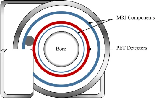
Figure 1.2 – Schematic of the Siemens Biograph mMR simultaneous
PET/MRI system ...5
Figure 1.3 – MR images (A) provide excellent soft tissue contrast for improved localization of PET images (B) as shown in the PET/MR
fusion image (C) ...6
Figure 2.1 – PET radiotracers consist of a bioactive molecule tagged with a radioisotope which decays by emitting a positron. The interaction of the positron with a surrounding electron produces two gamma
photons that are detected in PET ...9
Figure 2.2 – The detection of each pair of annihilation photons produces a line of response (red arrows). A particular line of response indicates that the underlying annihilation event (red circles) occurred
somewhere along that line ...11
Figure 2.3 – Photon attenuation (yellow) occurs as a result of interactions between annihilation photons and electrons in the surrounding tissue. This results in a loss of signal that degrades the accuracy
of the reconstructed PET image ...13
Figure 2.4 – Simulated PET images displaying the detrimental effect of
photon attenuation ...14
Figure 3.1 – The precession of a proton's magnetic moment around the magnetic field (A) is analogous to the precession of a spinning
top around the gravitational axis ...21
Figure 3.2 – After RF excitation, the magnetic moments of the spins (blue) produce a net magnetization vector (gold) in the xy-plane (A). Differences in the precession frequencies cause a dephasing effect
That lowers the net magnetization (red) (B) ...24
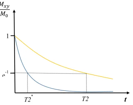
Figure 3.3 – The decay of transverse magnetization associated with T2* (blue)
is faster than the decay associated with T2 (gold) ...25
Figure 3.4 – The recovery of longitudinal magnetization associated with T1
xiv
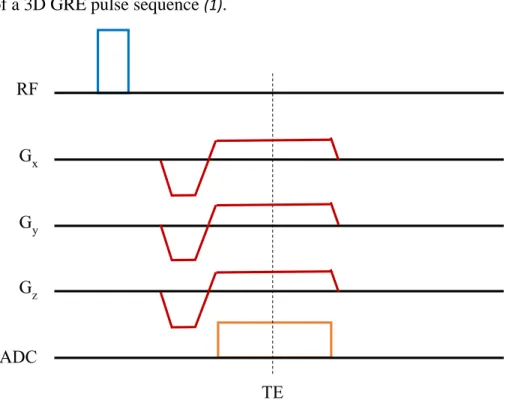
Figure 3.5 – Pulse sequence diagram for a conventional 3D GRE sequence ...28
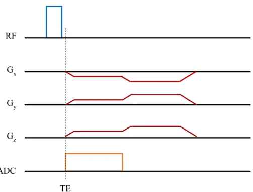
Figure 3.6 – Pulse sequence diagram for 3D UTE GRE sequence. ...30
Figure 4.1 – Representative flow chart for template-based MRAC methods ...33
Figure 4.2 – A flow chart of the derivation of pseudo CTs using the PASSR
method...34
Figure 5.1 – Sample slices from T1 (A) and CT (B) are shown here along with corresponding slices from R2* (C), Dixon-Fat (D), Dixon-
Water (E), and iUTE (F), respectively. ...44
Figure 5.2 – A mean R2* vs CT-HU scatter plot derived from 97 subjects
using a leave-one-out approach suggests a sigmoid relationship. ...47
Figure 5.3 – Representative segmentation results from one subject for the RiDR method (A) and vUTE method (B) overlaid on CT for bone (left) and air (right). True positives (yellow), false positives (green, overestimation), and false negatives (red, underestimation)
are shown ...53
Figure 5.4 – Sample slices from the μCT (A), μCAR-RiDR (B), and μvUTE (C)
attenuation maps from one subject in three orientations ...54
Figure 5.5 – Representative slices from percent-error maps from one patient show drastically reduced errors across the brain in PETCAR-RiDR (A)
compared to PETvUTE (B). Errors between ±1% are suppressed
for visual clarity ...55
Figure 5.6 – The lines-of-best-fit (red) displayed for a representative subject show that PETCAR-RiDR (A) approaches unity slope (green) when
regressed with PETCT whereas PETvUTE (B) displays
consistent underestimation. ...56
Figure 5.7 – Mean percent-errors computed in a variety of brain region ROIs show that the proposed method results in lower local errors than the vUTE method in all ROIs tested. The standard deviations at each ROI
(indicated by the error bars) are also much lower for the proposed method. ...57
Figure 6.1 – Images from spoiled GRE sequences (A) are not as affected by
susceptibility artifacts (arrow) as images from bSSFP sequences (B) ...67
Figure 6.2 – A plot of relative signal vs. flip angle is shown here for a TR = 9 ms. ...69
Figure 6.3 – The image on the left was acquired with 25,000 radial lines (A)
xv
Figure 6.4 – Regions in images acquired using the DUFA-UTE sequence
displayed signal loss in anterior portions of the head. ...73
Figure 6.5 – The iUTE3 image (A) displays large intensities in areas of bone (blue) and air (red), while the iUTE25 image (B) displays large
intensities in regions of csf (purple) and air (red). ...74
Figure 6.6 – The R1 image (A) and the R2* image (B) display large
intensities in areas of bone (red). ...75
Figure 6.7 – The R1 image (A) enables good separation of GM (red), WM (blue), and CSF (purple) while the R2* image (B) shows minimal
contrast between these tissues. ...76
Figure 6.8 – The Dixon1 (A), Dixon2 (B), and Dixon3 (C) images allow for
the refinement of adipose tissue (red) segmentation. ...77
Figure 6.9 – The scatter plot of mean R1 values vs. CT-HU values in bone
tissue shows a logarithmic relationship. ...77
Figure 6.10 – The scatter plot of mean R1 values vs. CT-HU values in brain tissue shows a piecewise linear relationship with separate conversions
for CSF (red), GM (blue), and WM (green). ...78
Figure 6.11 – The scatter plot of mean R1 values vs. CT-HU values in adipose
tissue shows a weak linear relationship. ...80
Figure 6.12 – Segmentation results from one subject using a CT-based method
(A), the TESLA method (B), and the vUTE method (C). ...82
Figure 6.13 – Segmentation results from one subject using a CT-based method
(A), the TESLA method (B), and the vUTE method (C). ...83
Figure 6.14 – Segmentation results from one subject using the TESLA method
(A) and the corresponding slice from the T1-MPRAGE image (B) ...83
Figure 6.15 – Sample attenuation maps shown from μCT (A), μTESLA (B),and μvUTE (C) ...85
Figure 6.16 – Sample percent-error maps for one subject for PETTESLA (A)
and PETCAR-RiDR (B) and PETvUTE (C). Errors within +/- 1%
are suppressed . Errors larger than +/- 20% were floored to +/- 20% ...85
Figure 6.17 – Voxel-wise scatter plots of PETCT vs. PETTESLA (A) and PETCT vs.
PETvUTE (B) brain voxel intensities from a representative subject are shown
here. The unity slope (green line) indicates a case with ideal correlation.
xvi
Figure 6.18 – Mean absolute percent-errors for PETvUTE (blue), PETCAR-RiDR (red),
and PETTESLA (orange) computed inside 24 ROIs. The error bars represent
one standard deviation of the mean. ...87
Figure 6.19 – Over-classifications of bone in the soft tissue regions of the sinuses is reduced in the TESLA method (B) compared to the
CAR-RiDR method (A). ...88
Figure 7.1 – A sample ADC-PET ratio image overlaid on an anatomical image shows regions of high ADC-PET ratio (blue) in lobe where the seizure
focus is present. ...98
Figure 7.2 – A representative slice from a representative attenuation map derived using the TESLA method show that regions of bone
and air are well identified. ...100
Figure 7.3 – Sample slices from PETDixon (A) and PETTESLA (B)
reconstructions for one patient show the presence of a hyper-metabolic lesion in the PETTESLA image that is
indiscernible in the PETDixon image (arrow). ...103
Figure 7.4 – A Dixon-based attenuation map derived for the pelvis region. ...104
Figure 7.5 – Slices in three orientations (left to right: coronal, sagittal, axial) from a TESLA-based segmentation derived for the pelvis region. The
xvii
LIST OF ABBREVIATIONS
AC Attenuation correction
ADC Apparent diffusion coefficient
bSSFP Balanced steady-state free precession
CAR-RiDR Continuous-valued attenuation coefficients from R2*-R2* and
iUTE-based segmentation with Dixon-iUTE-based refinement
CSF Cerebrospinal fluid
CT Computed tomography
CTAC Computed tomography-based attenuation correction
DCE Dynamic contrast-enhanced
DUFA-UTE Dual flip angle ultrashort echo time
DUTE Dual-echo ultrashort echo time
DWI Diffusion-weighted imaging
EEG Electroencephalogram
EM Expectation maximization
FA Flip angle
FDG Fluorodeoxyglucose
FOV Field-of-view
GM Gray matter
GRE Gradient recalled echo
HU Hounsfield units
IRB Institutional review board
xviii
iUTE inverse ultrashort echo time
IV Intravenous
LAC Linear attenuation coefficient
LOR Line of response
MAPE Mean absolute percent-error
MPE Mean percent-error
MPRAGE Magnetization-prepared rapid gradient-echo
MRAC Magnetic resonance imaging-based attenuation correction
MRF Markov random field
MRI Magnetic resonance imaging
MRS Magnetic resonance spectroscopy
OSEM Ordered subset expectation maximization
PASSR Probabilistic air segmentation and sparse regression
PET Positron emission tomography
RF Radiofrequency
ROI Region of interest
SD Standard deviation
SNR Signal-to-noise ratio
SPECT Single photon emission computed tomography
SUV Standardized uptake value
T1-MR T1-weighted magnetic resonance
TESLA T1-enhanced segmentation and selection of linear attenuation
coefficients
xix
vDixon Vendor-provided Dixon method
VFA Variable flip angle
vUTE Vendor-provided ultrashort echo time method
WASPI Water- and fat-suppressed proton projection imaging
WIP Work in progress
WM White matter
xx
LIST OF SYMBOLS
‖ ‖ Two-norm
α atlas patch weighting
β Positron
Bo Static magnetic field
B1 Radiofrequency magnetic field
e Euler’s number
18F Fluorine-18
ϒ Gyromagnetic ratio
GPE Phase-encoding gradient
GRO Read-out gradient
Gx Gradient in x-direction
Gy Gradient in y-direction
Gz Gradient in z-direction
1H Hydrogen nucleus
J Angular momentum
Kr Radial lines
λ1 Sparse regression term
λ2 Ridge regression term
L Thickness
μ Linear attenuation coefficient
xxi
MBq Megabecquerel
MHz Megahertz
M Magnetization vector
M0 Equilibrium magnetization vector
Mxy Equilibrium magnetization vector Mz Longitudinal magnetization vector
kev Kilo electron volts
kVp Peak kilo voltage
n Neutron
ν Neutrino
p Proton
ρ Proton density
Pt Template patch
PMR Patient patch
r2 Coefficient of determination
R1 Longitudinal relaxation rate
R2 Irreversible transverse relaxation rate
R2’ Reversible transverse relaxation rate
R2* Transverse relaxation rate
t Time
T Tesla
T1 Longitudinal relaxation time
xxii
T2’ Reversible transverse relaxation time
T2’ Irreversible transverse relaxation time
TE Echo time
TI Inversion time
TR Repetition time
1
CHAPTER 1: INTRODUCTION 1.1 Multimodality Imaging
The fundamental goal of medical imaging is to provide physicians with diagnostically
relevant images of the inside of a human body without the need for exploratory surgery.
Medical imaging systems are often classified either as anatomical modalities, which provide
structural information, or as functional modalities, which are used to study physiological
functions. Since they serve different purposes, anatomical modalities, such as magnetic
resonance imaging (MRI) and x-ray computed tomography (CT), have historically been
separated from functional modalities, such as positron emission tomography (PET). This
separation is evident in their placement in different clinical divisions (radiology and nuclear
medicine), but the advantages of integrating anatomical and functional imaging have been
recognized by clinicians for many decades. The primary benefit of combining these two types
of modalities is the ability to use anatomical images to localize any regions of functional
abnormalities. To this end, there are two general approaches which one can use to assimilate
information from functional and anatomical images: software and hardware (1).
1.2 Software-based Image Fusion
The first attempts at combining anatomical and functional images were made in the late
1980s and produced sophisticated image fusion software with the capability of aligning
functional images with separately-acquired anatomical images. These algorithms go beyond
simple image overlays or the use of external stereotactic frames either by identifying common
2
intensities in the images. For either approach, the complexity of the transformation needed
depends on the possible degrees of freedom between the two images. For anatomical regions
such as the brain where a change in size or shape between scans is not anticipated, simple rigid
body transformations are sufficient. More complicated nonlinear registration techniques are
needed when there are no constraints on the possible deformations. One example of this is in
the abdomen during non-rigid respiratory motion. Assessments of these methods have shown
that a local registration accuracy of approximately 2 mm can be achieved for the brain while
the performance is markedly worse for other regions of the body such as the lung and the
pelvis, where the local registration accuracy can be as poor as 5-8 mm. Therefore,
software-based solutions are limited to cases where image registration is trivial (1).
1.3 Hybrid PET/CT
In contrast, hardware approaches provide a simple and convenient approach to
combining images by integrating instrumentation from functional and anatomical modalities
and acquiring both sets of images in a common reference frame. The first of these hardware
approaches to be developed was the hybrid PET/CT scanner which acquires co-registered PET
and CT images in a single study (1). Hybrid PET/CT systems were commercially introduced
in 2001 and gained widespread acceptance among clinicians shortly thereafter, particularly in
oncology. PET is a functional imaging modality that allows clinicians to visualize complex
physiological processes such as metabolism, proliferation,perfusion, and receptor binding (2).
CT is an anatomical imaging modality that derives its contrast from the absorption or scattering
of the transmitted x-ray photons by tissues in the body, also known as photon attenuation.
Therefore, in addition to providing anatomical images to serve as a context for the functional
3
correcting for the phenomenon of gamma photon attenuation in PET. Details about the
phenomenon of photon attenuation as well as about CT-based attenuation correction will be
presented in Chapter 2.
Hybrid PET/CT systems are not without considerable drawbacks. First, CT imaging
employs the transmission of ionizing radiation in the form of x-rays through a patient’s body.
Although the doses associated with CT scans are low enough not to have any deterministic
effects, stochastic effects that result in elevated risk for developing cancer have been
demonstrated (3). Second, CT is limited in the imaging capabilities it can offer. For example,
simultaneous PET and CT acquisitions are not a realistic possibility nor are they desirable
because simultaneous acquisition would not provide much additional information compared to
sequential acquisition. Third, the contrast in CT imaging proves sufficient for some
applications, but is particularly lacking for most soft tissue applications. Specifically, the CT
images cannot be used to localize PET signals to gray matter or white matter regions of the
brain. Therefore, while the anatomical context and the ability to easily perform attenuation
correction are vast improvements over stand-alone PET systems, PET/CT systems leave much
to be desired.
A B C
4 1.4 Hybrid PET/MRI
Recently, hybrid PET/MRI systems have been developed to fill the voids left by
PET/CT scanners. While make-shift systems with MRI-compatible PET inserts are also in
existence, truly hybrid PET/MRI systems currently exist in two forms: sequential (Ingenuity
TF, Philips, Best, Netherlands) and simultaneous (SIGNA, General Electric,
Buckinghamshire, United Kingdom; Biograph mMR, Siemens, Erlangen, Germany). While
sequential systems address the concerns of ionizing radiation and lack of soft tissue contrast
expressed with PET/CT, simultaneous PET/MRI systems are generally preferable due to the
capability of acquiring information from both modalities simultaneously. References made to
PET/MRI systems hereafter in this dissertation refer to the Biograph mMR simultaneous
PET/MRI system manufactured by Siemens Healthcare (Erlangen, Germany) (4). PET/MRI
images presented in this work were acquired using a Biograph mMR system either at the
Biomedical Research Imaging Center at the University of North Carolina at Chapel Hill or the
Mallinckrodt Institute of Radiology at Washington University in St. Louis.
Developing a truly integrated system around the constraints imposed by the MRI
component’s strong magnetic field proved to be a difficult task. MRI instrumentation by
necessity contains no ferromagnetic metal components that could interfere with imaging
capabilities. However, existing PET detector technology is highly sensitive to the presence of
magnetic fields. Therefore, novel PET detector technology which could operate well under the
rigorous conditions imposed by the strong magnetic field utilized in MRI was developed. The
PET detectors were designed to be able to function in between two MRI components of the
system, as shown in Figure 1.2. These innovations were highly expensive, raising doubts about
5
simultaneous PET/MRI systems have been referred to as “a solution looking for a problem”
because they are a product of a technological advance rather than a solution for a pressing
clinical need (5).
The current consensus to the question of whether PET/MRI systems are worth the
markedly increased cost over PET/CT systems seems to be “perhaps”. However, simultaneous
PET/MRI systems are gaining support from researchers and clinicians in various fields,
especially for applications where anatomical images with excellent soft tissue contrast are
needed (Figure 1.3); MRI can also be used to gather physiological information about oxygen
metabolism, the structure of nerve and muscle fibers, and a plethora of other physiological
parameters (6), serving as an excellent complement to PET imaging.
In addition to potential clinical applications for PET/MRI systems that have already
been identified in neurology (7), cardiology (8), and oncology (9), there are also many technical
advantages to utilizing PET/MRI systems in lieu of existing hybrid PET/computed tomography
(CT) systems. As previously mentioned, there is no additional ionizing radiation incurred on PET Detectors
MRI Components
Bore
6
patients in order to obtain the anatomical information used to localize PET signals. In addition,
the anatomical information provided by MRI is far superior to that of CT, especially in the
realm of soft tissue contrast. Finally, MRI can be used to address existing technical issues in
PET including motion correction (10) and partial volume correction (11) that could not be
addressed using PET/CT systems.
Despite the many advantages, there is a major technical drawback with PET/MRI
systems: PET photon attenuation correction. Attenuation correction (Chapter 2) is
straight-forward in PET/CT due to the ease of utilizing the CT component of the system to derive the
necessary information; there is no analogous way to gather this information in PET/MRI
systems due to differences in the source of signal (Chapter 3). The focus of this dissertation is
on the development of potential approaches to perform MRI-based correction for PET photon
attenuation. Chapter 2 introduces the fundamentals of PET imaging and the physics of photon
attenuation, while Chapter 3 addresses the basics of MRI as well as its limitations in providing
the information necessary for PET attenuation correction. Chapter 4 explores existing methods
along with their strengths and pitfalls with particular emphasis on the current methods utilized
by the manufacturer. Chapter 5 presents an initial solution to the problem of MR-based
attenuation correction, while Chapter 6 outlines a more refined solution. Chapter 7 discusses Figure 1.3: MR images (A) provide excellent soft tissue contrast for improved
localization of PET images (B) as shown in the PET/MR fusion image (C).
7
certain clinical applications of PET/MRI systems and the relevance of the final attenuation
correction method to those applications. Chapter 8 serves as a conclusion for this dissertation
by outlining the contributions made by this dissertation to the field and by identifying areas
8
REFERENCES
1. Townsend DW. Multimodality imaging of structure and function. Phys Med Biol. 2008;53:R1-R39.
2. Bailey D, Townsend D, Valk P, Maisey M, eds. Positron Emission Tomography: Basic Sciences. London: Springer-Verlag London; 2005.
3. U.S. Food and Drug Administration. What are the risks of radiation from CT? 2015. Available from: http://www.fda.gov/RadiationEmittingProducts/RadiationEmittingProducts andProcedures/MedicalImaging/MedicalX-Rays/ucm115329.htm. Accessed June 10, 2015.
4. Delso G, Furst S, Jakoby B, et al. Performance measurements of the siemens mMR integrated whole-body PET/MR scanner. J Nucl Med. 2011;52:1914-1922.
5. Yankeelov TE, Peterson TE, Abramson RG, et al. Simultaneous PET-MRI in oncology: A solution looking for a problem? Magn Reson Imaging. 2012;30:1342-1356.
6. Haacke E, Brown R, Thompson M, Venkatesan R. Magnetic Resonance Imaging: Physical Principles and Sequence Design. 1st ed. New York: Wiley-Liss; 1999.
7. Barthel H, Schroeter ML, Hoffmann KT, Sabri O. PET/MR in dementia and other neurodegenerative diseases. Semin Nucl Med. 2015;45:224-233.
8. Rischpler C, Nekolla SG, Kunze KP, Schwaiger M. PET/MRI of the heart. Semin Nucl Med. 2015;45:234-247.
9. Bagade S, Fowler KJ, Schwarz JK, Grigsby PW, Dehdashti F. PET/MRI evaluation of gynecologic malignancies and prostate cancer. Semin Nucl Med. 2015;45:293-303.
10. Catana C. Motion correction options in PET/MRI. Semin Nucl Med. 2015;45:212-223.
9
CHAPTER 2: PHOTON ATTENUATION
2.1 Positron Emission Tomography
Positron emission tomography (PET) is a molecular imaging modality that allows
clinicians to visualize complex physiological processes such as metabolism, proliferation,
perfusion, and receptor binding. Due to this capability, PET has had a tremendous impact in a
number of fields including cardiology, neurology, psychiatry, and, most significantly, in
oncology where PET is routinely used for everything from the diagnosis of malignancies to
assessing treatment response of anti-cancer therapies (1).
The contrast in PET imaging is typically introduced through intravenous (IV) injection
of a molecular probe known as a radiotracer into the patient. These radiotracers are formed by
10
chemically combining the bioactive molecule of interest with a positron-emitting radioisotope.
As the radiotracer travels through the patient’s body and reaches the tissue or location of
interest, secondary detection of radioisotope decay (Figure 2.1) allows for the visualization of
the radiotracer distribution throughout the body.
Radioisotopes undergo spontaneous radioactive decay and is characterized by the
half-life, which represents the time it takes for half of the radioactive material present to decay, of
that isotope. Half-lives for radioisotopes of interest in PET range from 1.25 minutes (82Rb –
cardiac perfusion) to 100 hours (124I – thyroid imaging). The particular decay pathway that a radioisotope follows is determined by the cause for instability in the underlying atomic
nucleus. The nuclei of PET radioisotopes are proton-rich, i.e. the number of protons is too high
for the nuclei to be stable. These isotopes undergo decay by eliminating a proton from the
nucleus in order to rectify this imbalance. As shown in Equation 1, this correction most often
occurs through the transformation of a proton (p) to a neutron (n), releasing a positron (β) and neutrino (ν) in the process (1).
1
1p+ → 10n + 01β + ν (2.1)
While neutrinos pass through body tissue without any interactions, each positron
travels a short distance from its origin through the surrounding tissue, gradually dissipating its
kinetic energy as a result of collisions and scattering with tissue electrons and nuclei. This
distance, known as the positron range, depends on the initial energy of the positron at release
and is approximately 1-2 mm for positrons resulting from the decay of 18F atoms. When its
kinetic energy is nearly depleted, a positron undergoes an annihilation event with the next
electron it encounters. This annihilation event results in the production of radiation in the form
11
that these photons are emitted in anti-parallel directions, but the slightly non-zero momentum
possessed by the positron just prior to the annihilation event results in angles that are slightly
less than 180° (1).
2.2 Image Acquisition
Each pair of photons from an annihilation event travels through the patient’s body and
reaches the surrounding PET detector ring at approximately the same time, forming what is
known as a line-of-response (LOR). An LOR indicates a linear path along which the
annihilation event that produced the associated photons occurred (Figure 2.2). Due to
differences in the distances traveled by each photon in a pair, it is expected that the lag time
between the first photons reaching a detector and the second photon could be as long as 3 – 4
ns. Therefore, the window of time allotted for an LOR to form must be at least as wide as a
few nanoseconds. The collection of LORs produced over the course of the PET study is
organized in the form of a sinogram which is then reconstructed into an image corresponding
to the distribution of the radiotracer in the patient (1).
Figure 2.2: The detection of each pair of annihilation photons produces a line of response (red arrows). A particular line of response indicates that the underlying annihilation event (red circles) occured somewhere along that line.
12 2.3 Image Formation
Once the raw PET data is acquired, it can be reconstructed into a PET image using an
analytical approach (filtered back-projection) or an iterative approach (iterative
reconstruction). Iterative methods are preferable to analytical methods due to the improved
handling of noise and to the more realistic model of the system utilized. There are five basic
components to iterative reconstruction methods. The first component is a model for the image
to be reconstructed. This is simply the discretization of the image into a certain number of
voxels, or volume elements. The second component is a model of the imaging system that
contains probabilities that emissions of photons originating at a given voxel are detected in a
particular projection through that voxel. The third component is a model of the imaging data.
Since the formation of each LOR is a discrete process, a Poisson model is the most appropriate
choice. The fourth component is the governing principle of the method. This is the component
that defines what a “best” image is for a given set of PET data and is often expressed as a
mathematical cost function. In PET, the most common principle is the maximum likelihood
(ML) approach. The fifth component is the algorithm utilized to optimize the cost function.
The reconstruction algorithm employed by the manufacturer in the PET/MRI system is a
variant of expectation maximization (EM) algorithms called the ordered subset expectation
maximization (OSEM) algorithm (2).
2.4 Photon Attenuation
In an ideal world, all gamma photons resulting from the annihilation events would be
correctly accounted for by the PET detector system, allowing the reconstruction algorithm to
form a PET image that perfectly reflects the distribution of the radiotracer. In reality, there are
13
the detectors, causing a loss of signal that degrades the accuracy of the PET reconstructions
(Figure 2.3). These processes are collectively known as photon attenuation. Analytical
simulations (Figure 2.4) have shown that, if left uncorrected, photon attenuation can result in
errors of approximately 80% or higher in certain regions in the PET field-of-view. At PET
photon energy levels, there are two mechanisms through which photons are attenuated:
photoelectric effect (low probability) and Compton scattering (high probability) (1).
The photoelectric effect describes the interaction between an annihilation photon and
orbital electrons of atoms in the surrounding tissue. Through this interaction, the photon
transfers all of its energy to the electron, ejecting the electron from orbit. In this case, the
annihilation photon is eliminated and the underlying annihilation event is completely
undetected. The photoelectric effect dominates at photon energies of approximately 100 keV
and thus composes a very small percentage of the attenuation events at PET energy (511 keV).
The primary mode of photon attenuation in PET is through Compton scattering in which an
annihilation photon interacts with a loosely bound electron in a surrounding atom. The result Figure 2.3: Photon attenuation (yellow) occurs as a result of interactions between
annihilation photons and electrons in the surrounding tissue. This results in a loss of signal that degrades the accuracy of the reconstructed PET image.
14
of this interaction is a deflection of the photon’s path, along with a corresponding drop in the
photon's kinetic energy (1).
The deflected trajectory of some scattered photons still leads them towards the PET
detector ring where they are collected in a different detector than originally intended. If this
occurs within the coincidence time window, the resulting LOR does not accurately represent a
line along which the annihilation event occurred. This phenomenon is known as scatter. Some
scattered photons are deflected completely out of the range of the PET detector rings. This
phenomenon where the photons are not detected is known as attenuation (Section 2.3). This
distinction is important because the presence of scattered photons in the PET raw data
adversely affects image reconstruction. The attenuation correction component of PET
reconstruction assumes that scattered photons are removed from the data, a principle known as
the narrow-beam condition. Therefore, scattered photons must be identified and discarded prior
to performing attenuation correction. If scatter correction is not performed, the PET images
after attenuation correction will broadly overestimate the true PET signal (1).
There are various approaches that can be used to perform scatter correction. One
approach is to use energy windows to isolate scattered photons from photons unaffected by
scatter. Since scattered photons arrive at the detectors with less energy than unscattered 400
0
Corrected Uncorrected
PET Signal
15
photons, the energy of the detected photons can be used to identify the photons that have been
scattered (1). Another approach, which is utilized by the vendor to perform scatter correction
in PET/MRI, is known as single-scatter simulation (3). In this method, simulations are
conducted using seeds placed in the attenuation map (Section 2.5) generated for the patient in
order to estimate the amount of scatter along all possible LORs. These scatter estimates are
then subtracted from the acquired PET data to yield the scatter-corrected data. While scatter
correction itself is outside the scope of this dissertation, it is important to note that scatter must
be addressed prior to performing attenuation correction in order to satisfy the narrow-beam
condition. In addition, the scatter correction method utilized by the vendor employs the same
attenuation map as the routine for performing attenuation correction, which could result in a
compounding of errors if the attenuation map used is not sufficiently accurate.
2.5 Attenuation Correction
The basic principle behind attenuation correction is to estimate the percentage of
photons that are expected to be attenuated along any given LOR and to compensate for this by
modifying the PET raw data accordingly. In order to perform such a correction, knowledge of
the likelihood of attenuation along all possible LORs in the PET field-of-view is required. This
likelihood depends on both the linear attenuation coefficient (LAC), which is a function of
electron density, and the thickness of all tissues along a particular LOR. This attenuation
information is organized in the form of an attenuation map whose image intensities represent
the LAC values at all locations in the field-of-view. The equation for determining the fraction
of photons that are expected to be attenuated is shown in Equation 2.2, where μ represents the
LAC value, L represents thickness, and P/P0 represents the fraction of photons that are not
16
field-of-view is divided into equally sized voxels. This attenuation map is then integrated into
the OSEM reconstruction method to perform the correction for photon attenuation. The
primary challenge in attenuation correction lies in the measurement of tissue LAC values for
all regions in the PET field-of-view.
P
P0 = e-μL (2.2)
In stand-alone PET systems, this map of linear attenuation coefficients, referred to as a
μ-map, is acquired using a rotating radiation source that emits gamma photons which travel
through the patient’s body, similar to CT imaging. Since the number of photons emitted is
known and the number of photons detected can be measured, Equation 2.2 can be used to
compute the corresponding LAC values. However, the number of photons emitted by the
gamma source is relatively low, and a fairly long acquisition time is needed in order to achieve
an adequate signal-to-noise ratio (SNR) in the attenuation map. This difficulty in acquiring
attenuation maps was a major reason for the development of hybrid PET/CT systems and their
eventual replacement of stand-alone PET systems.
2.6 CT-based Attenuation Correction
In PET/CT systems, a quick CT scan provides an image that can be transformed and
used for PET attenuation correction (AC). CT systems utilize the attenuation of x-rays
transmitted through a patient’s body as the source of contrast and are also governed by
Equation 2.2. Therefore, CT inherently measures the physical parameter of interest in PET
attenuation correction, rendering it a logical choice to integrate with PET in order to provide
the necessary information. Prior to incorporation, a transformation of CT data is necessary due
to the energy dependence of linear attenuation coefficients. High energy photons such as the
17
such as the approximately 100 keV x-ray photons in CT. More details about the CT-based
attenuation correction (CTAC) method, which is regarded as the current gold standard for
performing AC in PET, are provided in Chapter 5.
2.7 MRI-based Attenuation Correction
While attenuation correction is fairly straightforward in PET/CT due to the relevant
information provided by the CT component of the system, this is not the case in PET/MRI
systems. MRI signals are primarily dependent on proton density and tissue magnetization
relaxation characteristics (Chapter 3); as a consequence, MRI does not directly provide the
measure of electron density necessary to correct for photon attenuation. Furthermore,
conventional MRI does not provide much information about the primary biological attenuator
of photons per unit volume in the human body: bone. In conventional MR images, bone and
air are virtually indistinguishable, but they possess LAC values that are on opposite ends of
the spectrum. Several studies have commented on the errors introduced into PET
reconstructions if bone is ignored in the attenuation map (4).
PET is very effective as a quantitative imaging modality, providing insight about
physiological functions by measuring the uptake of injected radiotracers. If this quantitative
advantage is to be maintained, errors in PET images, such as the ones produced through
inadequate attenuation correction, cannot be tolerated. Thus, development of an accurate
MRI-based correction for photon attenuation is paramount. There are existing methods (Chapter 4)
that seek to address this issue, but none of them has emerged as the standard for MRI-based
attenuation correction (MRAC). To understand both the limitations of MRI to this application
and, ironically, how the versatility of MRI can be used to produce an elegant solution to this
18 REFERENCES
1. Bailey D, Townsend D, Valk P, Maisey M, eds. Positron Emission Tomography: Basic Sciences. London: Springer-Verlag London; 2005.
2. Alessio A, Kinahan P. PET image reconstruction. In: Karesh S, Halama J, Wagner R, Zimmer A, Henkin R, eds. Nuclear Medicine, 2nd Edition. Elsevier; 2006.
3. Accorsi R, Adam LE, Werner ME, Karp JS. Optimization of a fully 3D single scatter simulation algorithm for 3D PET. Phys Med Biol. 2004;49:2577-2598.
4. Andersen FL, Ladefoged CN, Beyer T, et al. Combined PET/MR imaging in neurology: MR-based attenuation correction implies a strong spatial bias when ignoring bone.
19
CHAPTER 3: MAGNETIC RESONANCE IMAGING 3.1 Equilibrium Magnetization
Magnetic resonance imaging (MRI) was initially dubbed nuclear magnetic resonance
imaging, but the name was subsequently shortened due to the negative connotations attached
to the term “nuclear” during the Cold War era. This change is unfortunate since “nuclear”
precisely describes the particle being imaged in MRI: the atomic nucleus. In most cases, it is
the nuclei of hydrogen atoms (1H) in water molecules, which consist of a single proton, that
are of interest in MRI. Although other nuclei may also be used in MR, the 1H nuclei (hereby known simply as “proton”) are chosen due to the abundance of water in the human body and
because these nuclei exhibit non-zero nuclear magnetic moments arising from the spin of the
proton. Using classical physics, spin can be visualized as a rotation of the object about an axis,
but this explanation alone does not suffice to explain the origins of signal in MRI. Therefore,
some discussion in terms of quantum mechanics is required.
In quantum mechanical terms, spin provides particles with angular momentum and a
magnetic moment, both of which are expressed as vectors with discrete magnitudes and
orientations. While the orientation of a particle’s spin may change, the quantum number, i.e.
the magnitude, associated with it does not change. These spin quantum numbers start at ½ and
can exist in increments of 1 thereafter (ex: ½, 3/
2, 5/2 ...). The direction can be indicated as either
a positive or a negative spin number (ex: + ½ , - ½ ). The Pauli Exclusion Principle states that
two particles with the same spin number and orientation cannot exist in the same location. This
20
of spins for nuclei with even numbered protons and even numbered neutrons. Other nuclei,
such as the 1H nucleus, exhibit a non-zero spin because they contain an odd number of protons,
an odd number of neutrons, or both. This leads to a net nuclear spin for atoms with nuclei of
these compositions. Since the nucleus of a 1H atom contains a single unpaired proton, 1H exhibits a net spin of ½ and contains an angular momentum and a magnetic moment associated
with that spin. Equation 3.1 displays the relationship between the angular momentum (J) and the magnetic moment (μ). The term ϒ in Equation 3.1 is known as the gyromagnetic ratio. For
protons, 2πϒ = 42.58 MHz/T; for electrons, 2πϒ = 28,025 MHz/T (1).
μ = γ · J (3.1)
From this point on, a classical view of magnetism will used in lieu of a quantum
mechanical view for the sake of simplicity. In their natural state, the magnetic moments
associated with 1H nuclei in the human body are randomly oriented, resulting in a near-zero
vector sum of net magnetization. When a human is placed inside of a strong magnetic field,
such as the B0 field introduced by an MRI scanner, these individual magnetic moments align with the external field in either the low energy state (in the same direction as the external field)
or the high energy state (in the opposite direction). At room temperature, there is a slight
preference towards the low energy state, resulting in a non-zero bulk magnetic moment that
aligns with the external magnetic field. Since there is an abundance of water in the human
body, this bulk magnetic moment, known as the equilibrium magnetization, is large enough to
be manipulated and detected.
3.2 Precession
The vector sum of the magnetization at any given time is represented by a
21
of the B0 field, which is assumed to be the +z-axis without loss of generality. While M0 is aligned with the external magnetic field, the individual magnetic moments of the spins that
compose M0 precess about the B0 field (Figure 3.1A). This precession phenomenon arises due to the intrinsic angular momentum of the protons and is analogous to the precession of a
spinning top about the gravitational field of the earth. For instance, if a top is placed on a table
on its sharp end, it will topple over immediately. If the same top is spun about its axis prior to
release, the top will precess about the earth’s gravitational field until it loses a significant
portion of its angular momentum (Figure 3.1B).
The rate of spin precession about a static magnetic field is characterized by the Larmor
frequency (ω0). As shown in Equation 3.2, this frequency is a function of both the magnitude
of the static B0 field and the gyromagnetic ratio (1).
ω0 = γ · B0 (3.2)
3.3 Radiofrequency Excitation
The net magnetization M0 is constant and cannot be measured by the receiver coils because only time-varying magnetic flux that cut these coils can be detected. Therefore,
radio-z
x
y
B
0μ
J
A
B
z
x
y
J
F
G22
frequency (RF) pulses that are tuned to the Larmor frequency are used to tip, or rotate, the
magnetic moments of individual spins away from the direction of the main magnetic field.
More specifically, this RF pulse effectively rotates the M0 vector by an arbitrary flip angle (FA) away from the B0 field, producing a transverse component in the xy-plane, or transverse plane, (Mxy), and leaving part of the longitudinal component along the z-axis (Mz).
As a side note, electrons could theoretically be imaged using MR the way protons are
imaged, but the relationship in Equation 3.2 provides a biological limitation on imaging
electrons in the human body. Since the value of ϒfor electrons (Section 3.1) is much larger
than for protons, the Larmor frequency would also increase by that factor. This increase in
frequency requires RF pulses that deposit greater amounts of energy to achieve resonance, too
high in fact to safely use on humans.
After the RF pulse is applied and the rotation into the transverse plane is accomplished,
the magnetic moments of individual spins tend to realign themselves with the external
magnetic field in a process termed magnetization relaxation. To describe using the vector
notation introduced earlier, Mxy will tend to return to its initial value of zero while Mz will tend to return to its initial value of M0.
To summarize the process of acquiring signal in MRI, the net magnetization of all spins
is initially aligned with the external magnetic field before an RF pulse is used to rotate part or
all of the magnetization into the transverse plane. RF coils are then used to detect the electrical
signals induced as the transverse magnetization precesses about the z-axis.
The electrical signals produced in the RF coils are recorded in MR imaging space
known as k-space (more details in Section 3.6). The MR image is then most commonly
k-23
space data. The intensity at any given location in an MR image is a function of the
concentration of 1H nuclei (i.e. proton density) and the underlying chemical properties that
affect magnetization relaxation. There are two mechanisms through which magnetization
relaxation of MR signals occurs: transverse (Section 3.4) and longitudinal (Section 3.5).
3.4 Transverse Decay
As mentioned above, the transverse magnetization will tend to relax back to its initial
value of zero. This relaxation is also known as transverse decay because it describes the loss
of magnetization in the transverse plane that occurs as a result of the return to the equilibrium.
The first-order differential equation that governs the transverse relaxation process is shown in
Equation 3.3, where Mxy represents the component of the magnetization vector M in the transverse plane, while T2* and R2* respectively represent the time constant and the rate
constant for this exponential decay. Since they are reciprocals, T2* and R2* can be used
interchangeably to describe the transverse decay phenomenon.
dMxy dt =
-Mxy
T2* = -(Mxy) · R*2 (3.3)
Transverse decay occurs as a result of the dephasing (Figure 3.2) of the spins giving rise to
Mxy. This dephasing can result due to the inhomogeneity in the static field B0 and due to the interactions of spins with each other (1).
One mechanism for transverse magnetization decay is through B0 inhomogeneity. Slight variations in the static B0 magnetic field are caused by the presence of the patient inside the MRI scanner. As suggested by Equation 3.2, this inhomogeneity causes the precession
frequency to vary based on position. The differences in the precession frequencies, in turn,
cause the spins of interest to be out-of-phase with respect to each other, lowering the magnitude
24
by T2’ whereas the corresponding relaxation rate is denoted by R2’. This type of transverse
decay is known as reversible decay because certain RF pulses can be used to bring spins back
in-phase at a future time-point prior to signal acquisition.
Differences in precession frequencies can also occur due to spin-spin interactions.
Since individual spins impose their own individual magnetic moments, there exists a minute
magnetic field around each spin. The effect of the magnetic field of one spin on the surrounding
spins changes the magnetic field experienced by those spins, resulting in dephasing. This type
of transverse decay is known as irreversible decay because it cannot be reversed using MR
sequence techniques. The time constant associated with this relaxation is denoted by the
spin-spin relaxation time T2 while the corresponding relaxation rate is denoted by R2. T2 relaxation
is influenced by the underlying chemical structure. Values of T2 are much shorter for solids
(on the order of μs) and much longer for liquids (on the order of s).
The resulting transverse decay time (T2*) and the corresponding transverse relaxation
rate rate (R2*) can be computed as shown in Equations 3.4 and 3.5.
z
x
y
A
z
x
y
B
25
1 T2* =
1 T2+
1
T2' (3.4)
R*2 = R
2 + R'2 (3.5)
The evolution of Mxy as a result of the transverse decay is illustrated in Figure 3.3. The changes in the transverse magnetization observed are as seen in the curve associated with T2* decay unless an aforementioned technique is used to reverse the dephasing effects of B0 inhomogeneity (1).
3.5 Longitudinal Recovery
Longitudinal magnetization relaxation is also known as longitudinal recovery because
it describes the recovery of the magnetization along the longitudinal axis (parallel to the static
magnetic field). Equation 3.6 shows the first-order differential equation that governs the
longitudinal relaxation process, where Mz represents the component of the magnetization
𝑀
𝑥𝑦𝑀
0t
1
e
-1T2
*T2
26
vector along the longitudinal axis, T1 represents the time constant for this relaxation, and R1
represents the corresponding relaxation rate, illustrated in Figure 3.4.
dMz
dt =
M0-Mz
T1 = (M0-Mz) · R1 (3.6)
T1 and R1 are known as the spin-lattice relaxation time and the spin-lattice relaxation rate,
respectively, because the energy deposited by the RF excitation is dissipated into the
surrounding molecules, or the lattice (1). Since they are reciprocals, T1 and R1 can be used
interchangeably to describe the longitudinal recovery phenomenon.
3.6 Pulse Sequences and Image Acquisition
An MRI pulse sequence is the collective execution of system components in order to
achieve excitation and signal acquisition. One of the most basic sequences in MRI is the
gradient recalled echo (GRE) sequence. In a typical GRE-based sequence, RF excitation is
used to tip the magnetization of spins located in a particular volume of interest by a certain flip
angle from the longitudinal axis. After a short time passes and a certain amount of relaxation
𝑀
𝑧𝑀
0t
1
1- e
-1T1
27
occurs, signal is acquired from these spins and reconstructed into an MR image of that volume.
This MR signal, and consequently the resulting image, is a function of the number of spins
present in the volume, or proton density (ρ), and the relaxation phenomenon discussed in
Sections 3.4 and 3.5.
GRE pulse sequences can be used to acquire images in 2D, where the volume of interest
consists of a slice, or in 3D, where the volume of interest consists of a slab. In 2D imaging, the
slice to be acquired is isolated using magnetic gradient fields, known as the slice-select
gradient (GSS). These gradients slightly alter the static B0 magnetic field along a given axis. While this axis can be chosen to lie in any direction, the longitudinal axis (z) parallel to the B0 field is used most commonly. According to Equation 3.2, changing the B0 value along an axis
in a predictable manner causes the frequency of the spinning protons to exhibit a certain pattern
according to their position along that axis. The magnitude and the sign of this slice-select
gradient can be used to alter the Larmor frequency across the patient. The RF pulse, which is
tuned to the frequency corresponding to the slice of interest, is applied concurrently and,
depending on the desired flip angle, tips a certain percentage of the magnetization in that slice
to the transverse plane. Similarly, gradients applied in the transverse place, known as the
read-out gradient (GRO) and the phase-encoding gradient (GPE), are used to encode the frequency
based on location within each slice. A frequency domain table, termed k-space, is then built up
by changing GPE and GRO. Later, the k-space for each slice is transformed into an image using
the inverse 2D Fourier transform. Conventionally, the time from the center of the RF pulse to
the center of the acquisition window is known as the echo time (TE) because the spins will be
fully refocused at that time by the judicious use of the gradient waveform. The time between
28
In 3D MR imaging, the excited region consists of all of the spins in the field-of-view
of the RF transmitting coil. In the case of head and neck imaging, an RF coil would be used to
excite the region of the body superior to the shoulders. The three gradients, named after each
principal direction (Gx, Gy, and Gz), are then used to manipulate which part of the 3D k-space
is filled out with MR signal data. Once the acquisition is complete, the 3D k-space data is
transformed into a 3D image using the inverse 3D Fourier transform. Figure 3.5 illustrates an
example of a 3D GRE pulse sequence (1).
3.7 Shortcomings of MR in Attenuation Correction
In this chapter, the origin of MRI signals and their dependence on water proton density
and tissue magnetization relaxation characteristics has been described. As discussed in Chapter
2, the linear attenuation coefficients that reflect the probability of attenuation of PET photons
are a function of tissue electron density. A shortcoming of MR is that it cannot be used to safely
image electrons in vivo due to the tremendous amount of RF energy required (Section 3.3). RF
Gx
Gy
Gz
ADC
TE