Time Discounting and Credit Market Access in a Large-Scale
Cash Transfer Programme
Sudhanshu Handa1,2,4, Bruno Martorano3,4, Carolyn Halpern1, Audrey Pettifor1, and Harsha
Thirumurthy1
1University of North Carolina at Chapel Hill, Chapel Hill, NC 27599, USA
2Social & Economic Policy Section, UNICEF Office of Research—Innocenti, Florence, Italy 3Institute for Development Studies, Sussex University, Brighton, UK
Summary
Time discounting is thought to influence decision-making in almost every sphere of life, including personal finances, diet, exercise and sexual behavior. In this article we provide evidence on whether a national poverty alleviation program in Kenya can affect inter-temporal decisions. We administered a preferences module as part of a large-scale impact evaluation of the Kenyan Government’s Cash Transfer for Orphans and Vulnerable Children. Four years into the program we find that individuals in the treatment group are only marginally more likely to wait for future money, due in part to the erosion of the value of the transfer by inflation. However among the poorest households for whom the value of transfer is still relatively large we find significant program effects on the propensity to wait. We also find strong program effects among those who have access to credit markets though the program itself does not improve access to credit.
1. Introduction
Time preference, the relative importance individuals give to present versus future consumption, is a topic that has long captured the interest of economists. This interest is sparked by the belief that the time preference parameter is a crucial determinant of decisions in virtually every sphere imaginable, from risky sex to entrepreneurship, human capital investment and even obesity. The study of time preference has a long history in psychology where it is linked to self-control and emotional states (Damasio 1994; Bechara and Damasio 1997). In economics on the other hand the origins of time preference can be traced back to models of savings, growth and development (Rae 1905; Samuelson 1937; Smith 1776). More recently economists have begun to use both laboratory and small scale field
experiments to understand whether time preference affects financial decisions and the role of income or wealth in determining inter-temporal choice. This paper contributes to this literature using a large scale field survey in which households were randomly assigned to immediately enter into a national cash transfer program. The size of our sample and the fact that it comes from an actual program which currently reaches 170,000 households in Kenya
HHS Public Access
Author manuscript
J Afr Econ
. Author manuscript; available in PMC 2017 June 01. Published in final edited form as:J Afr Econ. 2016 June ; 25(3): 367–387. doi:10.1093/jae/ejv031.
A
uthor Man
uscr
ipt
A
uthor Man
uscr
ipt
A
uthor Man
uscr
ipt
A
uthor Man
uscr
implies a degree of external validity which distinguishes this study from previous work that relates economic circumstances to time discounting.
In the face of perfect capital markets the individual discount rate should converge to the market interest rate. However in developing countries such markets are far from perfect and so differences in individual discount rates may vary for that and other reasons as borne out in the empirical literature (Bradford et al 2014). For example there is evidence that the discount rate is affected by age (Handa et al 2014b), gender (Harrison et al. 2009), education (Perez-Arce, 2011), health (Handa et al 2014a), marital status (Bradford 2010) and even household size (Holden et al. 1998). The economics literature has been particularly interested in the role of income or wealth in determining inter-temporal choice and many analyses show that the poor discount more than the rich in both developed (Hausman, 1979; Lawrence, 1991; Harrison et al, 2002) as well as in developing countries (Pender and Walker, 1990; Yesuf and Bluffstone, 2008; Carvalho, 2010; Tanaka et al (2010); Holden, 2013), though there are some exceptions. For example, Ogaki and Atkeson (1997) argue that wealth and the discount rate are not correlated, Harrison et al. (2005) report that the discount rate decreased for Danish people reporting improvement in their economic conditions and Giné et al. (2013) do not find any relationship between shocks – proxied by a death of family members or an income shocks - and inter temporal choices.
A crucial question is why poverty conditions or negative income shocks shift preferences toward present gratification. According to one strand of the literature, the relationship between economic conditions and time preferences is mediated by neurobiological and psychological factors. In particular, poverty status could limit cognitive functions (Shah et al, 2012; Mani et al 2013) or augment stress leading people toward bad decisions (Chemin et al 2013; Cornelisse et al. 2013).1 Another explanation is that the poor discount more than the rich just because they cannot afford to do differently (Duflo, 2003). Indeed, since the subjective discount rate should not vary across the population under perfect capital markets, the role of credit constraints is considered to be a key factor determining inter-temporal choice in developing countries, and explaining the higher discount rates of the poor in particular (Holden et al. 1998; Yesuf and Bluffstone, 2008; Carvalho et al. 2014; Dean and Sautmann, 2014). This opens up the policy space for interventions to influence inter-temporal decision-making. Banerjee et al (2013) report evidence in this regard using randomized data from India, showing that women experiencing access to microcredit increase expenditure on durable goods and reduce expenditure on items associated with instantaneous utility. Haushofer and Shapiro (2013) show that people living in rural Kenya receiving a lump sum are more inclined to invest in durable goods while those benefitting from monthly transfers are present biased (i.e. are credit and saving constrained) while Handa et al (2013) find that an unconditional cash transfer program implemented in Zambia increases the propensity to wait for future money.
Building on the literature addressing the link between economic circumstances and inter-temporal choice, we investigate the impact of the Kenya Cash Transfer for Orphans and
1On the other hand, Handa et al (2013) show that a positive income shock increased subjective wellbeing which lead to a reduction of time discounting.
A
uthor Man
uscr
ipt
A
uthor Man
uscr
ipt
A
uthor Man
uscr
ipt
A
uthor Man
uscr
Vulnerable Children (CT-OVC) on beneficiaries’ time discounting using data that was collected for the evaluation of the CT-OVC. A special module on preferences and
expectations was administered during the 3rd wave of the evaluation to approximately 1800 respondents, one-third of whom were randomly assigned to a delayed entry control arm. In a companion paper (Handa 2014a), we present evidence on the experience in implementing these hypothetical and probabilistic questions in a large scale field survey in a poor population and show that the responses have rates of inconsistency that are quite low and similar to those found in laboratory experiments in highly literate populations. Building on this work, the aim of this paper is to investigate the interaction between receipt of the transfer and the position of individuals in the credit market. The cash transfer could
influence time preference by alleviating credit constraints and thus allowing beneficiaries to save and plan for the future. Alternatively an individual’s credit market position may itself be unaffected by the program but may act as a moderator, leading to a heterogeneous treatment effect whereby access to credit plus the additional cash available from the program together lead people to be more patient.
The paper thus contributes to the existing literature in several ways. Firstly, it provides evidence about the role of credit constraints in determining time discounting. Secondly, it is one of the few papers that investigate the impact of a national poverty alleviation program on time discounting and how that impact varies by the beneficiary’s credit market position. Finally, it is only one of two studies to investigate these questions within the context of a large scale national cash transfer program, thus contributing directly to the public policy literature on how poverty alleviation programs may affect time preference.
2. The Kenya CT-OVC
The Kenya CT-OVC reached 170,000 households and over 300,000 OVC across the country as of mid-2013 and is still expanding. The objective of the program, which began operating at scale in 2007, is to provide regular cash transfers to families living with orphans and vulnerable children (OVC) to encourage fostering and retention of children and to promote their human capital development. Eligible households, those who are ultra-poor (poorest 20 percent) and contain an OVC, receive a flat monthly transfer of $25 (U.S.) (KES2000 in 2015). An OVC is defined as a household resident between 0 to17 years old with at least one deceased parent, or who is chronically ill, or whose main caregiver is chronically ill.
Beneficiary households are informed that, in exchange for the cash payment, the care and protection of the resident OVC is their responsibility though there are no punitive sanctions for noncompliance with this responsibility.
Targeting of households for the program is conducted in three stages. In stage one each Location (a Location is the fourth administrative level below province, district and division) forms an OVC Committee (LOC) that prepares a list of all potentially eligible households in the Location that meet the demographic and poverty criteria. In stage two, the list of eligible households is sent to the program’s central office (located within the Ministry of Gender, Children and Social Development), which then administers a detailed socioeconomic questionnaire to assess poverty and confirm eligibility in order to rank households. The final number of households that enters the program in each district depends on funding to that
A
uthor Man
uscr
ipt
A
uthor Man
uscr
ipt
A
uthor Man
uscr
ipt
A
uthor Man
uscr
district, but approximately 20 percent of the poorest households in each Location are enrolled in the program. In cases where more households meet the eligibility criteria than funds are available, households are prioritized with child-headed households receiving the first priority (of which there are very few), followed by elderly-headed households.
3. Data and study design
Impact evaluation design
Prior to program expansion of the CT-OVC in 2007, UNICEF designed a social experiment to track the impact of the program on a range of household welfare indicators including food security, child health, and schooling. The evaluation entailed a randomized longitudinal design, with a baseline household survey conducted in 2007 and a 24-month follow-up in 2009. The ethical rationale for the design was that the program could not expand to all eligible Locations at the same time, so Locations whose entry would occur later in the expansion cycle could be used as control sites to measure impact. Within each of seven districts across the country (Kisumu, Homa Bay, Migori, Suba, Nairobi, Garissa, and Kwale), four Locations were identified as eligible, and two were randomized for immediate implementation and two were randomized for deferred expansion, serving as control Locations, for a total of 14 control and 14 intervention Locations. Targeting of households was carried out in all Locations according to standard program operation guidelines, and from the eligibility lists a sample of households was drawn, two-thirds from intervention Locations and the remaining third from control sites. Sample size was based on power calculations for the key impact indicators of school enrollment and household consumption expenditures. Results from the impact evaluation have been reported by the Kenya CT-OVC Evaluation Team (2012a, b).
In 2011, we returned to the households in the original evaluation sample that had been re-interviewed in 2009 and administered the same household survey plus an additional module covering preferences and expectations. The 2011 study was approved by the University of North Carolina IRB and the Kenya Medical Research Institute Ethics Review Committee.
Household attrition2
The initial study period coincided with a time of political turmoil in Kenya resulting from the disputed national elections in December 2007. Over 1000 people died and approximately 400,000 people were internally displaced at this time. Consequently, attrition between baseline and the first follow-up in 2009 was 17 percent and concentrated in Kisumu and Nairobi, the two Locations in the study that experienced the most election-related unrest. Attrition between the 2009 and 2011 rounds was only 5 percent. Table A1 in Appendix 1 shows means of selected demographic and poverty measures for households in each arm across the three waves. Means for these indicators were stable across the three waves despite the relatively high attrition rate between 2007 and 2009, indicating that the
representativeness of the sample remained intact.
2This section is based on Handa (2014a).
A
uthor Man
uscr
ipt
A
uthor Man
uscr
ipt
A
uthor Man
uscr
ipt
A
uthor Man
uscr
To further explore the potential for selective or differential attrition we estimated the probability of attriting between 2007 and 2009 using baseline values for the variables reported in Table 1. The only statistically significant variables out of the 26 total variables in this regression were the indicators for Kisumu and Nairobi, the number of residents age 12– 17, (log of) household size and unprotected water source. To assess whether there was any differential determinant of attrition between the two groups we re-estimated this model interacting each regressor with the indicator for intervention status. In only two cases (out of a possible 26) was there a statistically significant interaction effect (the indicator for residence in Kwale, and the number of residents age 6–11). Based on the stability of characteristics in each arm across the waves, the fact that the two most important determinants of attrition stem from residence in Kisumu and Nairobi, and the minimal differences in the determinants of attrition across arms, the threat of selective attrition appears minimal. The results on the determinants of attrition are reported in Handa et al. (2014a).
Baseline balance
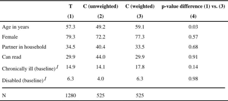
Table A1 in the Appendix compares mean poverty and selected demographic characteristics between treatment and control households at baseline. The set of poverty-related variables are balanced across arms in each wave, but there are differences in the age, sex and schooling levels of household heads across arms. This is due to the prioritization process that occurred at the central Ministry when the number of households selected by the communities for the program exceeded the budget. The prioritization process effectively gave weight to elderly-headed households. Since the final prioritization process was not conducted in control Locations (as they were not scheduled to enter the program immediately), households in the control arm of the study were sampled from the initial, slightly larger eligibility list than those from the intervention arm resulting in the differences in heads’ characteristics observed in Table A1. It is important to note however that there is no element of self-selection into the program; household eligibility was completely supply-driven and take-up was universal. Below we explain our method for addressing these differences in demographic characteristics.
4. Empirical strategy and measures
Empirical strategy
To measure the impact of the program on people’s time discounting, we estimate the following regression model:
(1)
where y defines individual time discounting, T the treatment status and X a set of control variables measured at both the individual (i) and household (h) level. The preferences module was administered to the main respondent of the household and as described above there are small differences in demographic characteristics across arms. To account for these differences we re-weight the control group sample using the method of inverse probability
A
uthor Man
uscr
ipt
A
uthor Man
uscr
ipt
A
uthor Man
uscr
ipt
A
uthor Man
uscr
weighting (IPW), which entails estimating the probability of being in the treatment group using a set of covariates measured at baseline, deriving the predicted probability and then weighting the control sample by the inverse of this probability. Since the prioritization criterion is known and based on age of the head, we ‘saturate’ this regression using eight 5-year age selection criterion Results of the estimating equation to derive the probabilities are available upon request; Appendix 2 reports the distribution of predicted probabilities before and after weighting which shows that the two distributions become much more similar after applying the weights. Table 1 reports means of selected characteristics of the respondents to the preferences module by study arm and as can be seen in Column (3), once the weights are applied the characteristics of the individual respondents in the control group move towards those of the treatment group with only the difference in mean age remaining statistically significant. In equation (1) we continue to include a full set of control variables to absorb this and any other difference between the two groups.
Inter temporal choice
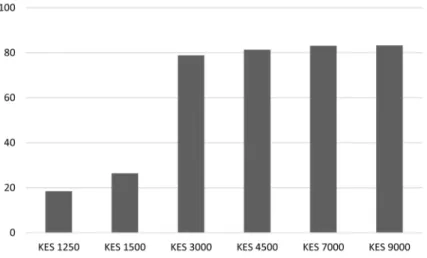
In order to measure time discounting, we invited participants to carry out an inter-temporal choice task entailing a decision between an immediate versus a future payment. While the former was fixed at KES 1500, the one month future values were varied as follows: KES 1500, 3000, 4500, 7000 and 9000 (Figure 1). We also included a KES1250 option as a check to see if people understood the question. Based on these responses we build two variables to capture impatience: an ordinal variable ranging from 1 (will wait for KES 1250) to 7 (will never wait for any amount) and a dichotomous variable indicating people who are never willing to wait for money.
Figure 1 reports the percentage of participants willing to wait for each option of payments. As expected, the percentage of participant that is willing to wait rises as the future value of the payment increases. Moreover, a substantial proportion of participants switch their preference from immediate money to future payments at KES 3000. Figure 1 also shows that more than 80 per cent of participants would wait one month for a future value of KES 9000, while about 16 per cent of people “always” prefer immediate money than future payments.
The order of the future value was randomized rather than listed in increasing value as in Holt & Laury (2002) and most laboratory or field experiments. We are thus able to identify inconsistent responses through ‘double-switches’, individuals who said they would wait for a low value and also said they will not wait for a higher value. Only eight per cent of respondents report a ‘double switch’ which is at the lower end of the inconsistency range found in controlled laboratory settings among wealthier, more literate populations (Bradford et al. 2014). About two-thirds of these inconsistent respondents are those who would wait for less money suggesting that they may not have understood this question. We exclude inconsistent respondents from our analysis but include those who would delay for less money; results are not sensitive to the exclusion of this latter group. Finally, the inter-temporal choice task that were administered in the survey was not incentivized--this is simply not feasible in a large multi-topic survey, both for financial reasons and because of time constraints. There is debate in the literature on whether reasonable answers can be elicited when tasks are not incentivized (Camerer and Hogarth, 1999; Harrison et al, 2007;
A
uthor Man
uscr
ipt
A
uthor Man
uscr
ipt
A
uthor Man
uscr
ipt
A
uthor Man
uscr
Delavande et al. 2011; Weisser, 2014), but the empirical evidence on the so-called hypothetical bias is mixed. Real games tend to use lower rewards for practical reasons, which confounds the evidence that hypothetical games lead to lower discount rates (more patience). In fact several studies have shown that hypothetical and real games lead to similar responses (Johnson and Bickel 2002; Holt and Laury 2002) and one study actually reports greater discount rates in a hypothetical game versus a real one (Harrison et al 2002).
Access to credit
In the 2011 survey we included a small set of questions on access to credit, capturing whether the household currently had any outstanding loans, whether they had sought a loan, and if they had not sought a loan, why not. We defined households as credit constrained if they had sought a loan and were rejected, or if they had not sought a loan for a reason that indicated they felt they could not obtain a loan (lack of collateral for example), or because they did not know where to go or how to get one (transaction cost constrained). As a result, about 3 out of 4 individuals in our sample are defined as credit constrained.
Figure 2 shows that the relationship between credit constrained and wealth (measured through a local linear regressions - lowess) is surprisingly flat except for very low levels of consumption (below KES 1000) and treated households appear slightly more credit constrained than control households. Note that credit constraints are measured 4 years after program implementation so these results suggest there was no program impact on credit constraints of households. The relatively flat relationship may be simply a function of the unique sample of households, all of whom are potentially eligible for the program and so are quite poor (mean consumption in the sample is 60 US cents per person per day).
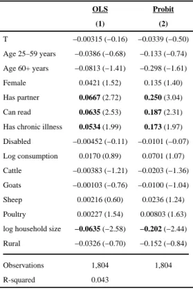
To investigate the determinants of access to credit we estimate regressions using a set of individual and household level covariates and also include treatment status—results are shown in Table 2 using OLS and probit specifications, both of which are weighted using the IPW. Having a partner in the household or being literate seem to be important determinants of credit access. In contrast, those living in larger households appear to be more credit constrained while individuals with a chronic illness are less so.
If credit constraints are an important determinant of time preference we might expect to see a relationship between our measure of credit access and the inter-temporal choice task we administered. Table 3 confirms that people without credit constraints appear more inclined to wait for future money. At every value of future money except for KES1250 (which is lower than the instantaneous option of KES1500) those with access to credit appear significantly more likely to wait (IES).
Mean comparisons between treated and control group
Beyond controlling for access to credit, the aim of this paper is to investigate the impact of the program on time discounting. Thus – as a first step – we compare the responses between participants in the program (treated group) and the others (control group) across the different payment options. As can be seen in Table 4, people in these two groups seem to respond in a similar way. The share of people willing to wait rises as the future value of the payment increases in both groups. A future value of KES 3000 represents a switch point in time
A
uthor Man
uscr
ipt
A
uthor Man
uscr
ipt
A
uthor Man
uscr
ipt
A
uthor Man
uscr
preferences for people in the treated as well as for those in the control group. Overall, the mean differences between these two groups are smaller than five points and statistically significant only for future values KES 9000, 4500 (at 10 per cent) and 7000 (at 5 per cent).
As before, we estimate local linear regressions to trace the relationship between propensity to wait and household wealth using (baseline) per adult equivalent household consumption. Figure 3 shows some evidence that even in this very poor sample, higher wealth is somewhat related to an increased propensity to wait for future money, and this pattern is stable across the two study arms. The proportion of households designated with access to credit is 22.5 percent in each arm.
We next check participant responses between treated and control group controlling for access to credit. As shown in Table 5, the mean differences are small and not statistically significant between treatment and control groups without access to credit. However differences are slightly larger between study arms among those having access to credit. Indeed, the mean differences are statistically significant for KES3000, KES 7000 (at 10 percent) and for the ordinal indicator of impatience.
5. Results
Full sample
Table 6 presents multiple regression estimates of the determinants of each of our 5 inter-temporal choice tasks. We also include estimates in the last 2 columns of the ordinal and dichotomous indicators for impatience described earlier. The first row of Table 6 indicates that beyond the threshold value of KES3000 individuals in the program display a 3–5 point higher likelihood of waiting for future money but this is statistically significant only for KES7000 and only at the 10 percent confidence level. Access to credit generally leads to a greater likelihood of waiting for future money, and less likelihood of never waiting no matter what the amount. Other results portray an interesting story about the determinants of inter-temporal decision-making. Literacy is strongly associated with delaying payment (by 8–9 points) while having a disability has an even stronger effect in the opposite direction, both intuitive results. In the Appendix we show results for the full sample, including the 8 percent of individuals who had inconsistent responses.
Results by baseline consumption levels
The weak relationship between the CT-OVC and time-discounting may in part be due to the relatively low value of the transfer at the third round when the preferences module was fielded. At baseline the value of the transfer as a share of beneficiary consumption was 23 percent. With inflation its value eroded to 18 percent in 2009 down to 11 percent by 2011. Consistent with the drop in the real value of the transfer, the significant impacts of the program on consumption (Kenya CT-OVC Evaluation Team 2012a) had dissipated by 2011 (Romeo, Dewbre et al 2014). It could be then that the weak effects of the program reflect in part the erosion in the ‘intensity of the treatment’, the fact that the transfer does not represent a large enough increase in income to alleviate liquidity constraints and induce an impact on the propensity to wait for future money.
A
uthor Man
uscr
ipt
A
uthor Man
uscr
ipt
A
uthor Man
uscr
ipt
A
uthor Man
uscr
We test this hypothesis by estimating program impacts on the poorest 50 percent of our sample, among whom median daily consumption is 34 US cents per person per day and the transfer share is 22 percent of baseline consumption. Results in the top panel of Table 7 show that in fact the program impact is about twice as high on this set of individuals than it is in the full sample and several of the point estimates are now statistically significant. For example the program increases the likelihood of waiting for KES 4500 or 7000 by 8 percentage points and reduces the ordinal impatience score by 0.392 (Table 7). The association between credit access and waiting for future money is also twice as high among this sample and also now statistically significant in several instances.
The bottom panel of Table 7 shows results for individuals in households with baseline adult equivalent consumption above the median for the sample. In contrast to the top panel of Table 8 here the program does not have any impact in delaying payment though access to credit does generally support individuals to delay payment, particularly for KES 7000 and 9000 and credit access significantly reduces the likelihood of never choosing to delay at any payment level.
Heterogeneous treatment effects by credit access
If liquidity constraints in the face of imperfect capital markets affect inter-temporal choice and the cash transfer itself is not big enough to eliminate liquidity constraints, than the cash transfer combined with credit access may together be large enough to overcome liquidity constraints and lead to impact on the choice task. We test this hypothesis by interacting the treatment dummy with the credit access variable. Initial estimates showed no differential impact by credit access among the control group so we drop the dummy variable for credit access (which measures the difference among the control group) and estimate the following model:
(2)
In this framework β2 measures the differential treatment effect by credit access among the
treated group only while the coefficient of the treatment dummy (β1) measures the
difference between the treated group without credit access and the entire control group. The constant term in this model shows the mean value of the dependent variable among the control group as a whole. Table 8 shows a significant heterogeneous treatment effect of the CT-OVC by credit access on the order of 6 percentage points with slightly larger effect sizes for larger values of future money. Moreover the difference between the treated group without credit access and the control group, given by the coefficient of the treatment dummy, is not significantly different. The two bottom panels of Table 8 show results by baseline adult equivalent consumption. These reveal that in fact for both groups, there is a positive treatment effect on the propensity to wait for future money in the presence of credit access with effect sizes of roughly equal magnitude. It seems then that the combination of the increased cash from the CT-OVC program and increased access to liquidity through the credit market work together to affect inter-temporal choice leading individuals to be more willing to wait for future money.
A
uthor Man
uscr
ipt
A
uthor Man
uscr
ipt
A
uthor Man
uscr
ipt
A
uthor Man
uscr
Using the model based on propensity to wait for KES7000 we show the predicted
probabilities of waiting for those with and without credit access among the treated group by baseline consumption. The program effect is about 6 points larger on average among those with credit access, but increases to almost 10 points at the top of the consumption
distribution, presumably where liquidity constraints are least binding.
6. Discussion and Conclusions
Liquidity constraints due in part to lack of access to credit are a major barrier to
consumption smoothing and investment in developing countries (Bardhan and Udry, 1999; Ghosh et al 2000; Rosenzweig and Wolpin 1993). Median consumption among households eligible for the Kenyan government’s largest poverty alleviation program is 60 cents per day and 77 percent are credit constrained. Program participation had an important initial impact on consumption, but this impact dissipated by the fourth year as the value of the transfer eroded with inflation. Our analysis shows that the program has only a weak positive impact on the propensity to wait for future money after four years. However this impact doubles in magnitude among the very poorest for whom the transfer still represents a relatively large portion of total consumption, suggesting that the transfer helps alleviate liquidity constraints and allows individuals to place more weight on the future. And when we focus on
individuals that are not credit constrained, we find large and statistically significant impacts of the program compared to households that are credit constrained. Among those with credit access the program increases the propensity to wait for KES3000 or more by 6 percentage points, and reduces the likelihood of never waiting for any sum of money by the same magnitude. Our interpretation of this effect is that the combination of the transfer and credit access is enough to relax the liquidity constraint for individuals and allows them to place more weight on the future.
Our results support the existing evidence that economic conditions or wealth affect inter-temporal choice though our study differs from the previous literature in that it is based on a large field study rather than a small laboratory or field experiment. The results reported here are exciting from a policy perspective, taken as they are from a rigorous impact evaluation of the Kenyan government’s largest poverty alleviation program. They imply that rather than any deficit in cognitive functioning, the way poor people perceive and discount their future is influenced by their environment and it is possible to promote forward looking decision-making by modifying these conditions through public policy. The results further show that a successful development intervention can achieve both equity and efficiency goals. In this example, an unconditional poverty targeted cash transfer program implemented on a large scale appears to be a win-win policy intervention: assuring social and economic protection on the one hand and promoting forward-looking decision-making on the other.
Acknowledgments
This research was funded by the U.S. National Institute of Mental Health through Grant Number 1R01MH093241 and by Eunice Kennedy Shriver National Institute of Child Health and Development R24 HD050924 to the Carolina Population Center.
A
uthor Man
uscr
ipt
A
uthor Man
uscr
ipt
A
uthor Man
uscr
ipt
A
uthor Man
uscr
References
Banerjee, AV. MIT Dept. of Economics Working Paper No. 02-17. 2001. Contracting Constraints, Credit Markets and Economic Development.
Banerjee, AV., Duflo, E., Glennerster, R., Kinnan, C. MIT Department of Economics Working Paper No. 13-09. 2013. The Miracle of Microfinance? Evidence from a Randomized Evaluation. Bardhan, P., Udry, C. Development microeconomics. Oxford University Press; 1999. Bechara A, Damasio H, Tranel D, Damasio AR. Deciding advantageously before knowing the
advantageous strategy. Science. 1997; 275:1293–1295. [PubMed: 9036851]
Bradford WD. The Association between Individual Time Preferences and Health Maintenance Habits. Medical Decision Making. 2010; 30:99–112. [PubMed: 19675322]
Bradford, WD., Dolan, P., Galizzi, MM. Looking Ahead: Subjective Time Perception and Individual Time Discounting. Centre for Economic Performance, LSE (No. dp1255); 2014.
Camerer CF, Hogarth R. The effects of financial incentives in experiments: A review and capital-labor-production framework. Journal of Risk and Uncertainty. 1999; 19:7–42.
Carvalho, L. RAND Working Paper Series WR- 759. 2010. Poverty and Time Preference.
Carvalho, L., Meier, S., Wang, SW. Poverty and economic decision making: evidence from changes in financial resources at payday. Center for Economic and Social Research Working Paper; 2014. Chemin, M., De Laat, J., Haushofer, J. SSRN scholarly paper ID 2294171. Social Science Research
Network; Rochester, NY: 2013. Negative rainfall shocks increase levels of the stress hormone cortisol among poor farmers in Kenya.
Cornelisse, S., Van Ast, V., Haushofer, J., Seinstra, M., Joels, M. SSRN scholarly paper ID 2294189. Social Science Research Network; Rochester, NY: 2013. Time-dependent effect of hydrocortisone administration on intertemporal choice.
Damasio, AR. Descartes’ error: Emotion, reason, and the human brain. New York: Putnam; 1994. Dean, M., Sautmann, A. Credit Constraints and the Measurement of Time Preferences. 2014. Available
at SSRN 2423951
Delavande A, Gine X, McKenzie D. Measuring subjective expectations in developing countries: A critical review and new evidence. Journal of Development Economics. 2011; 94(2):151–163. Di Falco, S., Damon„, M., Kohlin, G. Working paper. 2011. Environmental Shocks, Rates of Time
Preference and Conservation: A Behavioural Dimension of Poverty Traps?.
Duflo E. Grandmothers and granddaughters: Old-age pensions and intrahousehold allocation in South Africa. The World Bank Economic Review. 2003; 17(1):1–25.
Gine, X., Goldberg, J., Silverman, D., Yang, D. Revising Commitments: Field Evidence on the Adjustment of Prior Choices. mimeo; 2013.
Ghosh P, Mookherjee D, Ray D. Credit rationing in developing countries: an overview of the theory. Readings in the theory of economic development. 2000:383–401.
Handa S, Huang C, Hypher N, Teixeira C, Soares FV, Davis B. Targeting Effectiveness of Social Cash Transfer Programmes in Three African Countries. Journal of Development Effectiveness. 2012; 4(1):78–108.
Handa, S., Seidenfeld, D., Tembo, G. The Impact of a Large Scale Poverty Targeted Cash Transfer Program on Inter-temporal Choice. Carolina Population Center, University of North Carolina; Chapel Hill: 2013.
Handa, S., Martorano, B., Halpern, C., Pettifor, A., Thirumurthy, H. Innocenti Working Paper No. 2014-02. UNICEF Office of Research; Florence: 2014a. Subjective Well-being, Risk Perceptions and Time Discounting: Evidence from a large-scale cash transfer programme.
Handa, S., Martorano, B., Halpern, C., Pettifor, A., Thirumurthy, H. Working Paper. Carolina Population Center; 2014b. Time Discounting and age groups: Evidence from the Kenya Cash Transfer for Orphans and Vulnerable Children (CT-OVC).
Harrison GW, Morten IL, Melonie B. Estimating Individual Discount Rates in Denmark: A Field Experiment. American Economic Review. 2002; 92(5):1606–17.
A
uthor Man
uscr
ipt
A
uthor Man
uscr
ipt
A
uthor Man
uscr
ipt
A
uthor Man
uscr
Harrison, GW., Morten, IL., Rutström, EE., Melonie, B. Eliciting Risk and Time Preferences Using Field Experiments: Some Methodological Issues. In: Carpenter, J.Harrison, GW., List, JA., editors. Field Experiments in Economics. Greenwich: CT: JAI Press; 2005.
Haushofer, J., Shapiro, J. Household Response to Income Changes: Evidence from an Unconditional Cash Transfer Program in Kenya. Working Paper. 2013. available at: http://web.mit.edu/joha/www/ publications/haushofer_shapiro_uct_2013.11.16.pdf
Hausman JA. Individual Discount Rates and the Purchase and Utilization of Energy-Using Durables. The Bell Journal of Economics. 1979; 10(1):33–54.
Holden, S. CLTS Working Papers 8/13. Centre for Land Tenure Studies, Norwegian University of Life Sciences; 2013. High discount rates: - An artifact caused by poorly framed experiments or a result of people being poor and vulnerable?.
Holden ST, Shiferaw B, Wik M. Poverty, market imperfections and time preferences: of relevance for environmental policy? Environment and Development Economics. 1998; 3(1):105–130.
Holt CA, Laury SK. Risk aversion and incentive effects. American economic review. 2002; 92(5): 1644–1655.
Johnson MW, Bickel WK. Within-subject comparison of real and hypothetical money rewards in delay discounting. Journal of the experimental analysis of behavior. 2002; 77(2):129–146. [PubMed: 11936247]
Kenya CT-OVC Evaluation Team (Palermo et al.). Impact of the Kenya CT-OVC on Household Spending. Journal of Development Effectiveness. 2012a; 4(1):9–37.
Kenya CT-OVC Evaluation Team (Handa et al.). The Impact of the Kenya CT-OVC Program on Human Capital. Journal of Development Effectiveness. 2012b; 4(1):38–49.
Lawrance E. Poverty and the rate of time preference: evidence from panel data. Journal of Political Economy. 1991; 99(1):54–77.
Mani A, Mullainathan S, Shafir E, Zhao J. Poverty impedes cognitive function. Science. 2013; 341(6149):976–980. [PubMed: 23990553]
Meier S, Sprenger C. Present-biased preferences and credit card borrowing. American Economic Journal: Applied Economics. 2010; 2(1):193–210.
Ogaki M, Atkeson A. Rate of time preference, intertemporal elasticity of substitution, and level of wealth. Review of Economics and Statistics. 1997; 79(4):564–572.
Pender, JL., Walker, TS. Progress Report No. 97. Andhra Pradesh: ICRISAT; 1990. Experimental measurement of time preference in rural India.
Perez-Arce, F. RAND Working Paper Series WR- 844. 2011. The Effect of Education on Time Preferences.
Rae, JMCW. The Sociological Theory of Capital. New York: The Macmillan Co; 1905.
Romeo, A., Dewbre, J., Davis, B., Handa, S. Working paper. FAO; Rome, Italy: 2014. Consumption levels, inflation and human capital accumulation: Long term evidence from the CT-OVC social protection cash transfer programme of Kenya.
Rosenzweig MR, Wolpin KI. Credit Market Constraints, Consumption Smoothing, and the
Accumulation of Durable Production Assets in Low-Income Countries: Investments in Bullocks in India. Journal of Political Economy. 1993; 101(2):223–244.
Samuelson PA. A note on measurement of utility. The Review of Economic Studies. 1937; 4(2):155– 161.
Shah A, Mullainathan S, Shafir E. Some consequences of having too little. Science. 2012; 338(6107): 682–685. [PubMed: 23118192]
Smith, A. An Inquiry into the Nature and Causes of the Wealth of Nations. London: W. Strahan and T. Cadell; 1776.
Tanaka T, Camerer CF, Nguyen Q. Risk and Time Preferences: Linking Experimental and Household Survey Data from Vietnam. The American Economic Review. 2010; 100(1):557–571.
Yesuf, M., Bluffstone, R. Environment for Development Discussion Paper Series DP 08-16. 2008. Wealth and time preference in rural Ethiopia.
Warner J, Pleeter S. The Personal Discount Rate: Evidence from Military Downsizing Programs. American Economic Review. 2001; 91(1):33–53.
A
uthor Man
uscr
ipt
A
uthor Man
uscr
ipt
A
uthor Man
uscr
ipt
A
uthor Man
uscr
Weisser, RA. How ‘real’ is ‘hypothetical bias’ in the context of risk and time preference elicitation?. 2014. available at: http://www.aoek.uni-hannover.de/fileadmin/aoek/raw/
hypothetical_bias_working_paper_October_2014.pdf
Appendix 1
Table A1
Household characteristics by wave and intervention status in the CT-OVC Evaluation Sample
Sample: 2007 2009 2011
T C T C T C
Demographics
Household size 5.48 5.79 5.54 5.81 5.53 5.82
Female head 0.65 0.57 0.65 0.59 0.65 0.59
Age of head in years 62.34 56.06 62.21 56.20 62.55 56.55
Head not completed primary 0.53 0.38 0.53 0.38 0.53 0.38
Poverty
Per adult equiv. monthly exp. (Ks) 1533.30 1501.25 1541.77 1459.94 1550.14 1441.99
Walls of mud/dung/grass/sticks 0.75 0.84 0.75 0.86 0.74 0.87
Roof of mud/dung/grass/sticks 0.23 0.22 0.23 0.23 0.22 0.22
Floor of mud/dung 0.66 0.74 0.65 0.77 0.66 0.79
No toilet 0.55 0.56 0.55 0.56 0.54 0.56
Unprotected water source 0.62 0.68 0.61 0.70 0.61 0.70
Region
Garissa 0.10 0.06 0.11 0.06 0.09 0.05
Homa Bay 0.12 0.13 0.12 0.13 0.12 0.14
Kisumu 0.18 0.23 0.18 0.22 0.18 0.22
Kwale 0.08 0.09 0.08 0.10 0.08 0.11
Migori 0.23 0.23 0.22 0.25 0.22 0.26
Nairobi 0.13 0.10 0.13 0.07 0.13 0.06
Suba 0.15 0.16 0.16 0.16 0.17 0.17
N 1540 754 1325 583 1266 545
Statistically significant (at 10%) differences of t-test between Treatment (T) and Control (C) within each wave shown in bold. Thirty-three new households at follow-up not included in table.
A
uthor Man
uscr
ipt
A
uthor Man
uscr
ipt
A
uthor Man
uscr
ipt
A
uthor Man
uscr
Appendix 2
Figure A2.
Distribution of probability scores
A
uthor Man
uscr
ipt
A
uthor Man
uscr
ipt
A
uthor Man
uscr
ipt
A
uthor Man
uscr
Figure 1. Percent who will wait one month by future value
Note: the specific question was: “Suppose that you suddenly win money in the Lotto. If you could choose between these payment options which do you choose?”
A
uthor Man
uscr
ipt
A
uthor Man
uscr
ipt
A
uthor Man
uscr
ipt
A
uthor Man
uscr
Figure 2.
Relationship between household wealth and the probability of being credit constrained, by study arm
A
uthor Man
uscr
ipt
A
uthor Man
uscr
ipt
A
uthor Man
uscr
ipt
A
uthor Man
uscr
Figure 3.
Relationship between time preference and household wealth, by study arm
A
uthor Man
uscr
ipt
A
uthor Man
uscr
ipt
A
uthor Man
uscr
ipt
A
uthor Man
uscr
Figure 4.
Probabilities of waiting for those with and without credit access among the treated group by baseline consumption
A
uthor Man
uscr
ipt
A
uthor Man
uscr
ipt
A
uthor Man
uscr
ipt
A
uthor Man
uscr
A
uthor Man
uscr
ipt
A
uthor Man
uscr
ipt
A
uthor Man
uscr
ipt
A
uthor Man
uscr
ipt
Table 1
Mean characteristics of respondents of behavioral module
T C (unweighted) C (weighted) p-value difference (1) vs. (3)
(1) (2) (3) (4)
Age in years 57.3 49.2 59.1 0.03
Female 79.3 72.2 77.3 0.57
Partner in household 34.5 40.4 33.5 0.68
Can read 29.9 44.0 29.9 0.91
Chronically ill (baseline)1 14.9 14.1 17.8 0.14
Disabled (baseline)1 6.3 4.0 6.3 0.98
N 1280 525 525
1
A
uthor Man
uscr
ipt
A
uthor Man
uscr
ipt
A
uthor Man
uscr
ipt
A
uthor Man
uscr
ipt
Table 2
Determinants of the access to the credit
OLS Probit
(1) (2)
T −0.00315 (−0.16) −0.0339 (−0.50)
Age 25–59 years −0.0386 (−0.68) −0.133 (−0.74)
Age 60+ years −0.0813 (−1.41) −0.298 (−1.61)
Female 0.0421 (1.52) 0.135 (1.40)
Has partner 0.0667 (2.72) 0.250 (3.04)
Can read 0.0635 (2.53) 0.187 (2.31)
Has chronic illness 0.0534 (1.99) 0.173 (1.97)
Disabled −0.00452 (−0.11) −0.0101 (−0.07)
Log consumption 0.0170 (0.89) 0.0701 (1.07)
Cattle −0.00383 (−1.21) −0.0203 (−1.36)
Goats −0.00103 (−0.76) −0.0100 (−1.04)
Sheep 0.00216 (0.60) 0.0236 (1.24)
Poultry 0.00227 (1.54) 0.00803 (1.63)
log household size −0.0635 (−2.58) −0.202 (−2.44)
Rural −0.0326 (−0.70) −0.152 (−0.84)
Observations 1,804 1,804
R-squared 0.043
A
uthor Man
uscr
ipt
A
uthor Man
uscr
ipt
A
uthor Man
uscr
ipt
A
uthor Man
uscr
ipt
Table 3
Mean differences in per cent willing to wait by study arm and amount
Is willing to wait one month for KES: no access to credit access to credit p-value difference in means
1250 18.30 19.01 0.742
1500 25.25 30.28 0.046
3000 77.07 84.50 0.000
4500 79.75 86.38 0.001
7000 81.28 88.97 0.000
9000 81.35 89.44 0.000
Impatient: Ordinal 3.27 2.94 0.001
Impatient: Dichotomous 17.58 9.86 0.000
A
uthor Man
uscr
ipt
A
uthor Man
uscr
ipt
A
uthor Man
uscr
ipt
A
uthor Man
uscr
ipt
Table 4
Mean differences in per cent willing to wait by study arm and amount
Is willing to wait one month for KES: T C p-value difference in means
1250 19.1 19.5 0.84
1500 26.4 26.3 0.96
3000 78.4 75.0 0.13
4500 81.1 77.5 0.09
7000 83.1 78.7 0.03
9000 83.1 79.6 0.09
Impatient: Ordinal 3.2 3.3 0.14
Impatient: Dichotomous 16.0 19.2 0.11
N 1280 525
A
uthor Man
uscr
ipt
A
uthor Man
uscr
ipt
A
uthor Man
uscr
ipt
A
uthor Man
uscr
ipt
T ab le 5 Mean differences in per cent willing to w
ait by study arm and amount Not ha
ving access to cr
edit
Access to cr
edit
Is willing to wait one month f
or KES:
C
T
p-v
alue differ
ence in means
C
T
p-v
alue differ
ence in means
1250 21.98 19.07 0.237 11.16 19.1 0.026 1500 25.77 25.60 0.95 28.36 29.17 0.863 3000 74.99 76.71 0.505 74.80 84.03 0.032 4500 76.71 79.74 0.227 80.15 85.76 0.159 7000 77.51 81.35 0.119 82.79 89.24 0.083 9000 77.95 81.35 0.165 85.17 89.24 0.252 Impatient: Ordinal 3.34 3.25 0.471 3.34 2.97 0.046 Impatient: Dichotomous 20.64 17.64 0.21 14.34 10.42 0.262 N 386 992 1378 138 238 426
Control group mean weighted using the In
v
erse Probability W
A
uthor Man
uscr
ipt
A
uthor Man
uscr
ipt
A
uthor Man
uscr
ipt
A
uthor Man
uscr
ipt
T ab le 6Determinants of Propensity to W
ait for Future Mone
y
Is willing to wait one month f
or KES: Impatience 9000 7000 4500 3000 1500 Ordinal 1 Dichotomous 2 (1) (2) (3) (4) (5) (7) (9) T 0.0320 (1.17) 0.0459 (1.65) 0.0434 (1.52) 0.0471 (1.60) −0.00257 (−0.09) −0.176 (−1.31) −0.0320 (−1.17)
Access to credit
0.0603 (1.88) 0.0484 (1.44) 0.0357 (1.02) 0.0196 (0.52) 0.0272 (0.71) −0.157 (−0.99) −0.0603 (−1.88)
Age 25–59 years
0.0522 (0.89) 0.0483 (0.82) 0.0960 (1.51) 0.0656 (1.03) 0.0608 (0.96) −0.414 (−1.53) −0.0522 (−0.89)
Age 60+ years
0.0161 (0.27) 0.00997 (0.16) 0.0670 (1.02) 0.0461 (0.70) 0.0643 (0.96) −0.311 (−1.09) −0.0161 (−0.27) Female 0.0351 (0.80) 0.0294 (0.68) 0.0236 (0.53) 0.0339 (0.77) −0.0581 (−1.40) −0.00586 (−0.03) −0.0351 (−0.80) Has partner −0.0174 (−0.53) −0.0208 (−0.61) −0.0307 (−0.85) −0.0273 (−0.75) −0.0923 (−2.43) 0.228 (1.40) 0.0174 (0.53) Can read 0.0834 (2.49) 0.0887 (2.64) 0.0874 (2.56) 0.0944 (2.67) 0.0493 (1.27) −0.445 (−2.67) −0.0834 (−2.49)
Has chronic illness
−0.00789 (−0.18) −0.000595 (−0.01) 0.0123 (0.28) 0.0300 (0.67) 0.00887 (0.19) −0.0335 (−0.16) 0.00789 (0.18) Disabled −0.163 (−1.85) −0.155 (−1.77) −0.150 (−1.70) −0.145 (−1.62) −0.0932 (−1.57) 0.766 (1.89) 0.163 (1.85) Rural 0.0603 (0.89) 0.0557 (0.83) 0.0721 (1.08) 0.0890 (1.37) 0.0784 (1.41) −0.396 (−1.22) −0.0603 (−0.89) Log consumption −0.00786 (−0.32) −0.00219 (−0.09) 0.00510 (0.20) 0.00735 (0.28) 0.0280 (0.91) −0.0268 (−0.22) 0.00786 (0.32) Observ ations 1,664 1,664 1,664 1,664 1,664 1,664 1,664 R-squared 0.084 0.081 0.077 0.087 0.065 0.084 0.084
Notes: OLS re
gressions with rob
ust standard errors and in
v
erse probability weights; inconsistent responses e
xcluded. Also included in model b
ut not reported are indicators for district, log household size,
number of residents in each of six age cate
gories, quality of roof, floor
, w
alls, toilet f
acility
, type of cooking fuel used, electricity
, and cro
wding inde
x. Coef
ficients in bold are statistically signif
icant at 10
percent. 1 Higher v
alues indicate that indi
vidual needs increasingly higher amount of mone
y to w
ait.
2 W
ill ne
v
er w
ait for an
y amount of
A
uthor Man
uscr
ipt
A
uthor Man
uscr
ipt
A
uthor Man
uscr
ipt
A
uthor Man
uscr
ipt
T ab le 7Determinants of Propensity to W
ait for Future Mone
y by Baseline Consumption
Is willing to wait one month f
or KES: Impatience 9000 7000 4500 3000 1500 Ordinal 1 Dichotomous 2 (1) (2) (3) (4) (5) (7) (9) Belo
w median consumption
T 0.0601 (1.51) 0.0772 (1.88) 0.075 (1.79) 0.0746 (1.74) 0.0534 (1.43) −0.392 (−2.10) −0.0601 (−1.51)
Access to credit
0.0851 (1.93) 0.0697 (1.45) 0.0688 (1.42) 0.0436 (0.84) 0.121 (2.57) −0.43 (−2.02) −0.0851 (−1.93) Observ ations 824 824 824 824 824 824 824 R-squared 0.123 0.117 0.109 0.120 0.076 0.112 0.123 Abo v
e median consumption
T −0.00556 (−0.22) 0.00709 (0.27) 0.00696 (0.26) 0.0128 (0.45) −0.0582 (−1.81) 0.0691 (0.53) 0.00556 (0.22)
Access to credit
0.0586 (1.97) 0.0489 (1.62) 0.0249 (0.80) 0.0196 (0.60) −0.0173 (−0.46) −0.0703 (−0.47) −0.0586 (−1.97) Observ ations 841 841 841 841 841 841 841 R-squared 0.131 0.129 0.125 0.131 0.115 0.133 0.131
Notes: OLS re
gressions with rob
ust standard errors and in
v
erse probability weights; inconsistent responses e
xcluded. Also included in model b
ut not reported are indicators for Age 25–59 years, Age 60+
years, Female, Has partner
, Can read, Has chronic illness, Disabled, Rural, Log consumption as well as indicators for district, log household size, number of residents in each of six age cate
gories, quality of
roof, floor
, w
alls, toilet f
acility
, type of cooking fuel used, electricity
, and cro
wding inde
x. Coef
ficients in bold are statistically signif
icant at 10 percent.
1 Higher v
alues indicate that indi
vidual needs increasingly higher amount of mone
y to w
ait.
2 W
ill ne
v
er w
ait for an
y amount of
A
uthor Man
uscr
ipt
A
uthor Man
uscr
ipt
A
uthor Man
uscr
ipt
A
uthor Man
uscr
ipt
T ab le 8Interaction of treatment status and credit access on propensity to w
ait for future mone
y
Is willing to wait one month f
or KES: Impatience 9000 7000 4500 3000 1500 Ordinal 1 Dichotomous 2 (1) (2) (3) (4) (5) (6) (8) T 0.0180 (0.63) 0.0324 (1.11) 0.0325 (1.10) 0.0352 (1.15) −0.0112 (−0.36) −0.116 (−0.83) −0.0180 (−0.63)
T*access to credit
0.0594 (2.50) 0.0578 (2.43) 0.0463 (1.79) 0.0513 (1.87) 0.0368 (1.10) −0.259 (−2.09) −0.0594 (−2.50) Constant 0.548 (2.54) 0.506 (2.26) 0.292 (1.25) 0.231 (0.96) −0.131 (−0.51) 5.394 (5.11) 0.452 (2.09) Observ ations 1,664 1,664 1,664 1,664 1,664 1,664 1,664 R-squared 0.082 0.081 0.077 0.088 0.064 0.084 0.082 Belo
w median consumption
T 0.0438 (1.05) 0.0621 (1.45) 0.0634 (1.45) 0.0620 (1.39) 0.0288 (0.73) −0.294 (−1.50) −0.0438 (−1.05)
T*access to credit
0.0663 (1.83) 0.0625 (1.72) 0.0469 (1.21) 0.0541 (1.32) 0.101 (2.05) −0.405 (−2.19) −0.0663 (−1.83) Constant 0.969 (2.38) 0.901 (2.12) 0.67 (1.55) 0.846 (1.86) 0.0226 (0.05) 3.22 (1.64) 0.0314 (0.08) Observ ations 824 824 824 824 824 824 824 R-squared 0.118 0.114 0.105 0.119 0.068 0.108 0.118 Abo v
e median consumption
T −0.0204 (−0.59) −0.00776 (−0.22) −0.00618 (−0.17) −0.00113 (−0.03) −0.0558 (−1.26) 0.115 (0.64) 0.0204 (0.59)
T*access to credit
0.0641 (1.87) 0.0636 (1.85) 0.0556 (1.52) 0.0585 (1.50) −0.0106 (−0.23) −0.195 (−1.13) −0.0641 (−1.87) Constant 0.359 (0.87) 0.276 (0.65) −0.0692 (−0.15) −0.377 (−0.78) 1.021 (1.67) 5.102 (2.33) 0.641 (1.55) Observ ations 841 841 841 841 841 841 841 R-squared 0.129 0.129 0.126 0.133 0.114 0.134 0.129
Notes: OLS re
gressions with rob
ust standard errors and in
v
erse probability weights; inconsistent responses e
xcluded. Also included in model b
ut not reported are indicators for Age 25–59 years, Age 60+
years, Female, Has partner
, Can read, Has chronic illness, Disabled, Rural, Log consumption as well as indicators for district, log household size, number of residents in each of six age cate
gories, quality of
roof, floor
, w
alls, toilet f
acility
, type of cooking fuel used, electricity
, and cro
wding inde
x. Coef
ficients in bold are statistically signif
icant at 10 percent.
1 Higher v
alues indicate that indi
vidual needs increasingly higher amount of mone
y to w
ait.
2 W
ill ne
v
er w
ait for an
y amount of
A
uthor Man
uscr
ipt
A
uthor Man
uscr
ipt
A
uthor Man
uscr
ipt
A
uthor Man
uscr
ipt
T ab le A2Determinants of T
ime Discounting – full sample including inconsistent observ
ations
Is willing to wait one month f
or KES: Impatience 9000 7000 4500 3000 1500 Ordinal 1 Dichotomous 2 (1) (2) (3) (4) (5) (7) (9) T 0.0351 (1.34) 0.0436 (1.64) 0.0394 (1.45) 0.0373 (1.33) 0.00555 (0.19) −0.165 (−1.26) −0.0312 (−1.21)
Access to credit
0.0564 (1.84) 0.0445 (1.39) 0.0278 (0.84) 0.0195 (0.54) 0.0306 (0.81) −0.0614 (−0.41) −0.0489 (−1.62)
Age 25–59 years
0.0185 (0.33) 0.0121 (0.22) 0.114 (1.82) 0.0221 (0.36) 0.0597 (1.06) −0.273 (−0.96) −0.0254 (−0.46)
Age 60+ years
−0.0236 (−0.41) −0.0268 (−0.46) 0.0747 (1.14) 0.00589 (0.09) 0.0606 (1.01) −0.164 (−0.53) 0.0114 (0.20) Female 0.0408 (0.98) 0.0282 (0.69) 0.0229 (0.54) 0.0378 (0.90) −0.0618 (−1.56) −0.112 (−0.54) −0.0402 (−0.98) Has partner −0.0253 (−0.82) −0.0115 (−0.36) −0.0263 (−0.79) −0.0159 (−0.47) −0.0839 (−2.29) 0.136 (0.87) 0.0106 (0.35) Can read 0.0828 (2.68) 0.0803 (2.62) 0.0769 (2.44) 0.0910 (2.80) 0.0305 (0.80) −0.442 (−2.73) −0.0765 (−2.51)
Has chronic illness
0.00170 (0.04) 0.00799 (0.19) 0.0249 (0.59) 0.0383 (0.89) 0.0149 (0.34) −0.101 (−0.48) 0.00270 (0.06) Disabled −0.152 (−1.78) −0.157 (−1.84) −0.148 (−1.74) −0.143 (−1.65) −0.0888 (−1.55) 0.813 (2.10) 0.164 (1.93) Rural 0.0647 (1.02) 0.0616 (0.97) 0.0928 (1.48) 0.0940 (1.52) 0.0572 (1.09) −0.510 (−1.63) −0.0646 (−1.01) Log consumption −0.00894 (−0.40) −0.000786 (−0.03) −0.00531 (−0.22) 0.00307 (0.12) 0.0307 (1.08) −0.00582 (−0.05) 0.00981 (0.44) Observ ations 1,804 1,804 1,804 1,804 1,804 1,804 1,804 R-squared 0.078 0.077 0.075 0.080 0.059 0.077 0.079
Notes: OLS re
gressions with rob
ust standard errors and in
v
erse probability weights. Also included in model b
ut not reported are indicators for district, log household size, number of residents in each of six
age cate
gories, quality of roof, floor
, w
alls, toilet f
acility
, type of cooking fuel used, electricity
, and cro
wding inde
x. Coef
ficients in bold are statistically signif
icant at 10 percent.
1 Higher v
alues indicate need increasingly higher amount of mone
y to w
ait.
2 W
ill ne
v
er w
ait for an
y amount of