5573.pdf

(1)

MARGINALIZED ZERO-INFLATED POISSON

REGRESSION

Dorothy Leann Long

A dissertation submitted to the faculty of the University of North Carolina at Chapel Hill in partial fulfillment of the requirements for the degree of Doctor of Philosophy in the Department of Biostatistics.

Chapel Hill 2013

Approved by:

(2)

c

(3)

Abstract

DOROTHY LEANN LONG: Marginalized Zero-inflated Poisson Regression

(Under the direction of Dr. Amy H. Herring and Dr. John S. Preisser)

The zero-inflated Poisson (ZIP) regression model is often employed in public health research to examine the relationships between exposures of interest and a count out-come exhibiting many zeros, in excess of the amount expected under sampling from a Poisson distribution. The regression coefficients of the ZIP model have latent class in-terpretations, which correspond to a susceptible subpopulation at risk for the condition, with counts generated from a Poisson distribution, and a non-susceptible subpopulation that provides the extra or excess zeros. The ZIP model parameters, however, are not well suited for inference targeted at overall exposure effects, specifically, in quantifying the effect of an explanatory variable in the overall mixture population. We develop a marginalized ZIP model for independent responses to model the population mean count directly, allowing straightforward inference for overall exposure effects and easy accom-modation of offsets representing individuals’ risk times, as well as empirical robust variance estimation for overall log incidence density ratios. Through simulation stud-ies, the performance of maximum likelihood estimation of the marginalized ZIP model is assessed and compared to existing post-hoc methods for the estimation of overall effects in the traditional ZIP model framework. The marginalized ZIP model is applied to a recent study of a motivational interview-based safer sex counseling intervention, designed to reduce unprotected sexual act counts. Also, we develop a marginalized ZIP model with random effects to allow for more complicated data structures. SAS macros are developed for the marginalized ZIP model for independent data to assist applied

(4)

(5)

To my wonderful parents, you have always believed in me and encouraged me to pursue my dreams. To my fantastic husband Dustin, we both know this dissertation would have never happened without your loving patience, support, and encouragement. To Charlie, your smiles and unconditional love brighten every single day.

(6)

Acknowledgments

Most importantly I would like to thank my dissertation advisers. John Preisser has provided not only the ingenuity behind this work, but he has also given invaluable advice and guidance that have made me a better researcher. Through her outstanding mentoring and leadership, Amy Herring has been my strongest advocate, giving sage advice, offering much-needed encouragement, and challenging me to reach my full po-tential. I am extremely fortunate to have both Amy and John guide my work, both providing inspiration for the researcher I hope to be.

I would like to thank Dr. Suchindran, both for taking a chance on a pair of students from Tennessee and being so generous and supportive through my time at UNC. I would also like to thank my committee members, Carol Golin, Brian Neelon, and John Stamm, for their support and helpful comments which greatly improved this document. Also, I am very appreciative of the SafeTalk study team and participants for allowing me to work with and for them.

In addition to the support I have received from Dustin, I would like to thank several of my fellow classmates; Jennifer Clark, Annie Green Howard, Beth Horton, Andrea Byrnes, Elena Bordonali, and Matt Wheeler have all been sources of strength and comfort when coursework (and life) became overwhelming. Additionally, I could always depend on Melissa Hobgood for help, or words of wisdom, no matter the issue. You all will never know how truly vital you have been to my graduation.

(7)

T32ES007018 (NIEHS), R01-MH069989, DK56350, and AI50410.

(8)

List of Tables

2.1 Marginalized ZIP Performance with 10,000 Simulations and Varying Sample Size . . . 33

2.2 Comparison of Relative Median Biases for Estimation of Overall Expo-sure Effects with Marginalized ZIP, ZIP with Delta Transformation, ZIP with Na¨ıve Interpretations, & Poisson . . . 34

2.3 Comparison of Coverage Probabilities for Estimation of Overall Expo-sure Effects with Marginalized ZIP, ZIP with Delta Transformation, ZIP with Na¨ıve Interpretations, & Poisson . . . 35

2.4 Comparison of Power for Estimation of Overall Exposure Effects with Marginalized ZIP, ZIP with Delta Transformation, ZIP with Na¨ıve In-terpretations, & Poisson . . . 36

2.5 Marginalized ZIP Model Results: SafeTalk Example . . . 37

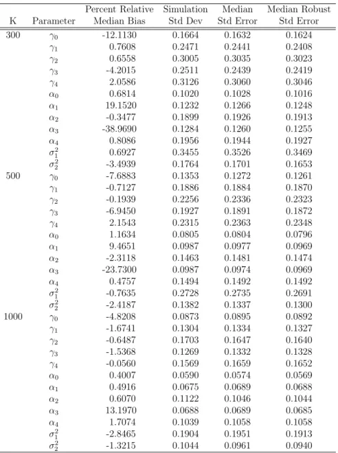
3.1 Marginalized ZIP w/ RE Performance with 1,000 Simulations and Vary-ing Number of Subjects . . . 54

3.2 Percent Relative Median Bias, Coverage & Power for Estimating Time 2 IDR (exp(α2)) and log-IDR (α2) . . . 55

3.3 Marginalized ZIP Model with Random Effects Results: SafeTalk Example 56

4.1 m ZIP Macro Output: Model-based Results . . . 66

4.2 m ZIP Macro Output: Robust (Empirical) Results . . . 67

4.3 m ZIP Macro Output: Odds Ratios for Zero-inflated Parameters γ . . . 68

4.4 m ZIP Macro Output: Incidence Density Ratios (IDR) for Marginal Mean Parameters α. . . 69

(11)

4.6 m ZIP Macro Output: Robust (Empirical) Covariance Matrix . . . 71

(12)

List of Figures

2.1 Histogram of UAVI Counts . . . 31

2.2 Standardized Pearson Residuals of SafeTalk Marginalized ZIP and Tra-ditional ZIP Models . . . 32

(13)

Chapter 1 Literature Review

1.1 Motivation

(14)

substandard products have a separate distribution. Many such examples of zero-inflated count data stem from the presence of multiple underlying unique populations, where factors that distinguish these separate populations are often latent.

In public health, much research is performed with the intent of understanding the incidence of a health event and its relationship with some exposure(s) of interest. In dental research, suppose an investigator is interested in the incidence of dental caries among children and determining whether the incidence depends upon a number of covariates. Due to some underlying set of confounders such as household fluoride levels or genetic factors, many children have no dental caries present at screening and would perhaps represent a subpopulation of those not susceptible to the condition of interest. On the other hand, the children who are at risk for caries have counts, not necessarily strictly positive, of dental caries and represent a subpopulation of subjects that might have a different distribution than those children not at risk. However, often data that are zero-inflated can arise from one homogeneous population where the notion of latent subpopulation categorization is not meaningful. In the dental caries example, researchers might not believe that a subpopulation of insusceptible children is clinically meaningful and might desire inference on the entire sampled population. Despite the exact nature of the inference desired, investigators have several options for statistical analyses of zero-inflated data.

1.2 Zero-Inflated Methods

(15)

Poisson (ZIP) regression model and the hurdle model. The hurdle model employs a binomial process to model all the zero counts, and then positive realizations are modeled through a truncated-at-zero count distribution. In the dental caries example, the hurdle model would describe those children with no caries separately from all the children who had any caries. Instead of modeling all the zero observations in the first process, the ZIP model models the ‘excess zeros’ in binomial process and then a count distribution is fit using a full Poisson likelihood. The ZIP model allows for zeros to occur within the distribution of a second population. In terms of dental caries, the zero-inflated Poisson model describes the ‘excess zero’ children, perhaps those not at risk of caries, separately from all those children susceptible to caries, but not necessarily with observed dental caries. We will explore these two methods in the following sections.

1.2.1 Zero-Inflated Models

Lambert (1992) introduces the concept and some theory behind ZIP regression mod-els, using a motivating example on solderability of boards (an experiment at AT&T). The ZIP model allows for modeling of the zeros in two ways, first the ‘excess’ zeros and then the zeros which occur in the Poisson distribution, which may occur for different reasons. The type of zero observed (excess or Poisson) is a latent variable. For Yi,

i= 1, . . . , n, the ZIP data are structured

Yi ∼

      

0 with probability ψi

Poisson(µi) with probability 1−ψi

(16)

yielding

Yi =

      

0 with probability ψi+ (1−ψi)e−µi

k with probability (1−ψi)e−µiµki/k!, k∈ Z+.

For the ith _subject, _ψ

i is the probability of being an excess zero and µi is the mean of

the non-excess zero population. To model these parameters of ψi and µi, we define

logit (ψi) = Ziγ

log (µi) = Xiβ

whereγ = (γ1, . . . , γp1)

0_,_β _{= (}_β

1, . . . , βp2)

0 _and_Z

i, Xi are (1×p1) and (1×p2) vectors of covariates for the ith unit. The log-likelihood for the ZIP model can be

l(β,γ|y) = X

yi=0

log heZiγ₊_e−eXiβ

i

+X

yi>0

(yiXiβ−eXiβ)

−

n

X

i=1

log (1 +eZiγ₎₋X

yi>0

log (yi!).

In the ZIP model, the parametersγ and β have latent class interpretations; that is, γj

is the log-odds ratio of a one-unit increase in thejth _{element of}_Z

i on the probability of

being anexcesszero andβj is the log-incidence density ratio of a one-unit increase in the

jth _{element of} _X

i on the mean of the suspectible sub-population. No simple summary

of the exposure effect on the overall mean of the outcome is directly available. Lambert admits that ZIP regression is difficult to interpret when the set of covariates affectψ,µ

and the mean number of defectsE(Yi) = (1−ψi)µi differently. That is, an explanatory

(17)

Lambert identifies that there are two model situations: one in which ψ and µ are unrelated and another in which ψ can be defined as a function of µ. Lambert examines the maximum likelihood estimation of the ZIP model parameters through the EM algorithm. For the special case whereψ is defined as a function of µ, Lambert suggests using the Newton-Raphson algorithm. Since the complete data log-likelihood can be separated into function of γ and β alone, then one can maximize over these separately using the EM algorithm, where the complete data log-likelihood is

lc(β,γ|y,z) = n

X

i=1

{(ziZiγ−log (1 +eZiγ)) +

(1−zi)(yiXiβ−eXiβ)

−(1−zi)log (yi!)}

= lc(γ|y,z) +lc(β|y,z)− n

X

i=1

(1−zi)log (yi!).

Herezi is latent class indicator of whether the ith observation originates from the zero

process (zi = 1) or the Poisson process (zi = 0). Exploiting the mixture structure

of the zero-inflated Poisson model, the EM algorithm iteratively fits weighted versions of simpler generalized linear models (Hall and Zhang, 2004). For large sample sizes, Lambert notes the MLE’s for the ZIP model parameters are consistent and following a normal distribution with means (γ,β) and variances equal to the inverse of the observed information matrices.

Adapting Lambert’s ZIP regression model, Hall (2000) formulates the zero-inflated binomial regression model to handle bounded count data and also expands the ZIP and binomial models to include cluster random effects. After briefly summarizing the zero-altered (hurdle) models, Hall discusses how the ZIP is preferable due to its inter-pretability and suitability for many types of data. For the example of pesticide efficacy on reducing the number of Whitefly, the parameters associated with the logistic model

(18)

quantify the effects of covariates on the probability that the pesticide is fully effec-tive, and the parameters in the Poisson process explain the association between the covariates and the mean number of insects occurring when the pesticide is not fully effective. Hall argues that both sets of parameters are scientifically meaningful, either when tested jointly or separately. In the derivations, Hall discusses Lambert’s EM al-gorithm for estimating the ZIP model parameters and notes that solving the M step via unweighted logistic regression is more straightforward than the weighted logistic regression on an augmented data set proposed by Lambert. With either method, both Lambert and Hall agree that the ZIP regression model is ‘not hard to fit.’

To account for correlated observations, Hall proposes including a random effect in the count model portion of the zero-inflated Poisson and binomial models. Specif-ically, let Y = (Y₁0, . . . ,Y_K0) where K is the number of independent clusters and Yi = (Yi1, . . . , YiTi)

0 _and _T

i is the number of observations for the ith cluster. Then

Yij ∼

      

0 with probability pij

Poisson (λij) with probability 1−pij.

where ψij is the probability of being an excess zero and µij is the mean of the

non-excess zero population for theith_{cluster and}_jth _{observation. The log-linear and logistic}

regression models are

logit(ψij) = Zijγ

log(µij) = Xijβ+σbi

where b1, . . . , bK i.i.d.

∼ N(0,1), Zi and Xi are the design matrices for the logistic and

(19)

effects can be expressed

l(θ,y) =

K X i=1 log Z ∞ −∞

" _T_i Y

j=1

Pr(Yij =yij|bi)

#

φ(bi) dbi

whereθ = (γ0,β0, σ), φ is the standard normal probability density and

Pr(Yij =yij|bi) =

ψij + (1−ψij)e−µij

uij

"

(1−ψij)e−µijµ yij

ij

yij!

#1−uij

= (1 +eZijγ₎−1

(

uij

eZijγ _{+ exp(−}_eXijβ+σbi₎ + (1−uij)

exp[yij(Xijβ+σbi)−eXijβ+σbi]

yij!

)

where uij = I(yij = 0). In order to handle the complexity of the estimation in this

situation, Hall employs the EM algorithm with Gaussian quadrature with the complete data log-likelihood

lc(θ;y,z,b) = logf(b;θ) + logf(y,z|b;θ)

=

K

X

i=1

logφ(bi) + K X i=1 Ti X j=1

{[zijZijγ−log(1 +eZijγ)]

+ (1−zij)[yij(Xijβ+σbi)−eXijβ+σbi −log(yij!)]]}

with zij being the latent indicator of whether Yij comes from the zero state (zij = 1)

or the Poisson(µij) state (zij = 0). Hall applies the proposed ZIP with random effects

to two data sets, one with pesticides and Whitefly larvae and also the Wiring Board data from Lambert (1992).

On the basis of marginal models and the general estimating equations (GEE) litera-ture, Hall and Zhang (2004) propose an alternative expectation-maximization approach

(20)

to incorporate within-cluster correlation. Using a dependence working correlation ma-trix, Hall and Zhang alter the M step of the EM algorithm by replacing the weighted GLM score equation with the weighted GEE, accounting for the correlation among subjects. This work builds on the works by Rosen et al. (2000) and generalizes the EM algorithm to the ES, expectation-solution, algorithm, which gives both consistent and asymptotically normal parameter estimators under regularity conditions. Hall and Zhang recognize the need to address selection methods for the appropriate working cor-relation structure for the ES algorithm, but the authors note efficiency, not consistency, of the parameter estimators would be affected.

Beyond accommodating repeated measures data, Gilthorpe et al. (2009) outline extensions of the ZIP and binomial models to account for over-dispersion through zero-inflated negative binomial (ZINB) and beta-binomial models. In addition, these au-thors discuss the negative implications of excluding covariates from the zero process (ie. latent class membership prediction) without significant consideration. Except for randomization-based arguments, it is doubtful that balanced zero counts exist across the Poisson process covariates, since this would imply the proportion of excess zeros to be equal across all combinations of covariates. Gilthorpe et al. also discuss methods for choosing between zero-inflated and generic mixture models.

(21)

predicted value approach and the direct approach, particularly for the ZINB and zero-inflated beta-binomial distributions.

In the average predicted value (APV) approach, individual predicted response val-ues under each binary exposure status xi are calculated then averaged to obtain the

estimated overall mean E(y|x, w). The APV can provide either an average difference in predicted responses or average ratio of expected values. First, the model-predicted responses are calculated for each individual (such as ˆµi = ˆψiˆλi in ZINB), both as if the

person was exposed (xi = 1) and as if they were unexposed (xi = 0), leaving all the

other covariates,wi, fixed at that person’s observed values. Then the average difference

in predicted responses is

θD ≡

Z

[E(yi|xi = 1,wi)−E(yi|xi = 0,wi)]dF(w)

where F(w) is the joint distribution function for the covariates wi in reference

popu-lation.

The next challenge is defining this joint distribution of the covariates. The authors suggest either assuming an appropriate distribution, based on the types of covariates used, or employing the empirical distribution function (EDF). For the parametric ap-proach, Albert et al. suggest using a multinomial distribution for categorical variables and either normal or multivariate normal distributions for continuous covariates. Em-ploying the observed data, one can also leave the covariate distributions unspecified and use the EDF; this method is averaging exposure effect over the EDF of the covariates. In ZINB for an individual i with covariates wi and exposure status x, we have

E(yi|xi,wi) = logit−1(α0+α1xi+α0wi) exp(β0+β1xi+β0wi)

(22)

and

θD =

1

nG

X

i∈G

{logit−1_{( ˆ}_α

0+ ˆα1+αˆ0wi) exp( ˆβ0+ ˆβ1+βˆ0wi)−logit−1( ˆα0+αˆ0wi) exp( ˆβ0+βˆ0wi)}

for group G of size nG. This estimator has the form of the ‘standardization formula’

from Hern´an and Robins (2006). This method uses model-predicted values to perform a stratified analysis within a subpopulation looking for observed differences between exposed and unexposed groups. Depending on how the distributions of the covariates differ between the exposed and unexposed groups, the APV may require some extrap-olation beyond the multivariate support of the data. If the ratio of expected values is desired instead of the average difference in responses, the authors provide

θR≡

R

E(y|x= 1,w)dF(w)

R

E(y|x= 0,w)dF(w).

The variances for ˆθD and ˆθR can be estimated through the delta method or the

boot-strap. The bootstrap has the added benefit of providing confidence intervals without requiring distributional assumptions. Also, depending on the form of the covariates, the delta method can be computationally intensive and tedious.

In addition to the APV, Albert et al. also present the ‘direct’ option of using a log-linear model for the probability of an excess zero (ψi) instead of logistic regression.

Thus the ZINB (log-log) models are

log(ψi) = γ0 +γ1xi+γ0wi

log(µi) = β0+β1xi+β0wi.

(23)

versus non-exposed) is

θRL ≡

µ1

µ0

= exp(γ0+γ1+γ

0_w

i) exp(β0+β1+β0wi)

exp(γ0+γ0wi) exp(β0+β0wi)

=eγ1+β1

While this approach is fairly simple and the variance of its estimator can be found using the delta method, it is limited by the appropriateness of the log-linear model for the first-step of the ZI model. In particular, the log-linear model is not limited to the range of 0-1 for predicted probabilities. The authors analyze dental caries data by the exposure of very low birth weight compared to normal birth weight, noting that the ZINB (logit-log), ZINB (log-log), and ZIBB (logit-logit) models produced the lowest AIC and BIC, with ZINB (log-log) model performing the best.

Through simulation studies, Albert et al. explore properties of their methods under correct and incorrect model selection, as well as for unbalanced covariate distribution across the exposure groups. An interesting fact is that even when the log-linear link was incorrect, the direct approach appeared to provide valid inference and was fairly robust; however, when the covariates were unbalanced, this method can be substantially biased, especially when the covariate has a large effect on the outcome.

While Albert et al. provide methods for producing estimates of overall exposure effects, the APV and ‘direct’ approaches are not straightforward and require either distributional assumptions on the extraneous covariates or the use of a log link for the excess zero process. Preisser et al. (2012) reviewed ZIP model usage in the dental caries literature and found that many health researchers have imprecise or misleading conclusions due to the complexity of the ZIP latent class structure.

(24)

1.2.2 Hurdle & Zero-Altered Models

Instead of modeling two latent class subpopulations, analysts can choose to use the hurdle model, which models all zeros separately from positive realizations, outlined by Mullahy (1986). In general, let φ1(y, θ1) and φ2(y, θ2) be two functions defined on

y∈Γ ={0,1,2, ...} satisfying φ1, φ2 >0 and

φ1(0, θ1) +

X

y∈Γ+

(y, θ2) = 1

where Γ+ = Γ− {0}. Note that a standard data model specifies φ1(y, θ1) = φ2(y, θ2) for all y∈Γ so that

X

y∈Γ

φ1(y, θ1) =

X

y∈Γ

φ2(y, θ2) = 1

The hurdle model occurs when a binomial probability governs whether a count variable has zero or positive realization. If the realization is positive, then the ‘hurdle’ is crossed and the conditional distribution of the positives is governed by a truncated-at-zero count data model. The probability that the threshold is crossed is Φ1(θ1) =

P

y=0φ(0, θ1), and the conditional distribution of the positives is φ2(y, θ2)/Φ2(θ2), where Φ2 is the summation ofφ2 on the support of the conditional density and the truncation normal-ization. Thus, the density function of y is

p(y) = [ P(y= 0)]I(y=0)∗[ P(y|y >0) P(y >0)]I(y>0) = [1−Φi(θ1)]I(y=0)∗[(φ2(y, θ2)/Φ2(θ2))∗Φ1(θ1)]I(y>0)

The likelihood can be expressed

L(θ1, θ2) = exp(ΛH) =

Y

t∈Ω0

[1−Φ1(θ1)] Y

t∈Ω1

(25)

where Ω0 = {t|yt = 0}, Ω2 = {t|yt > 0}, Ω = Ω0 ∪ Ω1 and ΛH represents the log-likelihood of the general form of the hurdle model. Mullahy notes that when Φ1(θ1) = Φ2(θ2), the likelihood reduces to

L(θ1, θ2) =exp(ΛH) =

Y

t∈Ω0

[1−Φ2(θ2)]

Y

t∈Ω1

[φ2(y, θ2)]

Mullahy then states that the specifications whereθ1 =θ2are of primary interest and de-rives the likelihoods for hurdle models for both the Poisson and geometric distributions, and affirming that the hurdle model can be extended to any count data model.

Building upon the hurdle model approach to modeling zero-inflated counts, Heilbron (1994) recommends using the same distribution to describe both sub-populations by using a truncated-at-one count distribution to model the zero observations and then the truncated-at-zero count distribution for the positive values. This method, referred to as the zero-altered count model, differs from the hurdle model by requiring that both processes have the same distribution and link functions. Let p1(y|λ1) represent the probability density function for the ‘standard’ sub-population andp2(y|λ2) represent the probability density function for the ‘zero’ sub-population. Then by lettingω=p2(0|λ2), the distribution is

f(0) = ω+ (1−ω)p1(0|λ1)

f(k) = (1−ω)p1(k|λ1), k > 0.

The zero-altered model is a hurdle model with additional assumptions: (1) p1 and

p2 have identical distribution forms and overdispersion parameters, (2) the covariates {Xj}and link functionsηk for modeling the meansλkof the distributions are the same

for the two parts (that is,ηk=β0k+Pp_j₌₁Xjβjk, k= 1,2), and (3)λ1 is a function of

λ2 and ancillary parameters. Heilbron proposes the relationship between λ1 and λ2 as

(26)

λ1 =γ1λ

γ2

2 , whereγ1 >0, γ2 ≥0, which implies β2j =γ2βj1, j ≥1.

Heilbron affirms that interpretations of parameter estimates is simple for the zero-altered model. First, equality of all corresponding coefficients βj1 = βj2 in the zero-altered Poisson model reduces to standard GLM based on p1. Additionally, the differ-ence (βj2−βj1) may be interpreted in terms of a difference in the meanλ1 or in other features of p1. The added-zero probability reduces top1(0|λ2)−p1(0|λ1) with overdis-persion parameters being the same in both terms. Distributions p1 where p1(0|λ) is decreasing inλ(such as Poisson and negative binomial) then the added-zero probability is positive if and only ifλ2 < λ1.

It is the zero-altered Poisson model that Dobbie and Welsh (2001) modify to uti-lize general estimating equations to account for correlated observations, and Min and Agresti (2005) further extend it in the repeated measures setting through the use of random effects.

In the context of both the zero-inflated Poisson and hurdle models, Neelon, O’Malley and Normand (2010) detail the fitting of zero-inflated models for repeated measures using Bayesian techniques. By incorporating prior information, the Bayesian approach to fitting these models has the added benefit of straightforward estimation of functions of parameters.

1.3 Marginalized Models

(27)

the conditional mean. When comparing population-averaged and subject-specific coef-ficients, Heagerty argues that the conditional regression coeffecients have limited utility. For the marginalized logistic-normal model, the author adopts a pair of regression mod-els, with the first focusing upon a population-averaged interpretation,

logit E(Yij|Xij) = Xijβ,

and the second model incorporating the dependence among the longitudinal observa-tions

logit E(Yij|bi,Xi) = ∆ij +bij

where bi = (bi1, . . . , bini)

0 _and _b

i|Xi ∼ N(0,Di). Here Di is a covariance matrix that

can be obtained as a function of observationti and the parameter vector α. Note the

parameter ∆ij is a function of ηij = Xijβ, the marginal linear predictor, as well as

σij =

p

var(bij), the standard deviation of the random effects, where

h(ηij) =

Z

h(∆ij +σijz)φ(z)dz,

h = logit−1 and φ is the standard normal probability density. Using both numerical integration and the Newton-Raphson iteration, ∆ij is found, given (ηij, σij). Since ∆ij

is a function of both β and α, Heagerty uses a 20-point Gauss-Hermite quadrature to solve the above convolution equation.

Merging some of the ideas of marginalized models and zero-inflated count methods, Lee et al. (2011) focus upon the hurdle model formulation of handling Poisson and negative binomial data with excess zeros while marginalizing over random effects for clustering. Let Yi = (Yi1, . . . , YiNi)

0 _{be the count response, where} _Y

it is the response for

theithindividual at timet, and letYitbe conditionally independent givenbi = (bi1, bi2)0.

Also, letXitbe the covariates pertaining toYit. The marginalized Poisson hurdle model

(28)

is given by

P(Yit=yit|Xit) =

      

1−pM_it if yit= 0

pM_it g(yit;λMit)

(1−e−λMit₎ if yit= 1,2, . . . , . where logit(pM

it) = X

0

itγ, g(yit;λMit) = e

−λM_it₍_λM

it)yit/yit!, and λMit = exp(X

0

itβ). To

account for the clustered nature of the responses, Lee et al. (2011) draw from Heagerty (1999) to create the conditional hurdle model

P(Yit =yit;bi) =

      

1−pC

it(bi1) if yit = 0

pC it(bi1)

g(yit;λC it(bi2))

(1−e−λCit(bi2)₎ if yit = 1,2, . . . , . where logit(pC

it(bi1)) = ∆it1 +zij0 1bi1,

g(yit;λCit(bi2)) =e−λ

C

it(bi2)₍_λC

it(bi2))yit/yit!,

log(λC

it(bi2)) = ∆it2 +zij0 2bi2 and bi = (bi1, bi2)

i.i.d.

∼ N(0,Σ). Here, zit1 and zit2 are subsets of Xit and

Σ=

  

Σ1 Σ12

Σ12 Σ2

  

where Σ1, Σ12 and Σ2 are unknown positive-definite matrices. Here ∆it1, ∆it2 are subject-specific intercepts and are functions of the marginal parameters (γ,β) and the dependence structure Σ. However, these γ and β are reported to have ‘marginal’ terpretations while handling the mixed model extension. Note that these ‘marginal’ in-terpretations are not ‘overall’ inin-terpretations; the parameterization of the hurdle model implies that γk quantifies the effect of a kth covariate on being an excess zero and βk

(29)

Chapter 2 A Marginalized Zero-inflated

Poisson Regression Model

2.1 Introduction

Zero-inflated count data exist in many areas of medical and public health research. Because Poisson regression is often inadequate in describing count data with many ze-ros (B¨ohning et al., 1999), Lambert (1992) proposed the zero-inflated Poisson (ZIP) regression model, based on a mixture of a Poisson distribution and a degenerate distri-bution at zero. The ZIP model has two sets of regression parameters that have latent class interpretations, one for the Poisson mean and the other for the probability of being an excess zero. These latent classes are often thought to classify someat-riskand not-at-riskpopulations, indicating a difference in susceptibility between the two groups. Others have extended Lambert’s model to cluster-specific random effects (Hall, 2000) and marginal models for clustered data (Hall and Zhang, 2004). A separate but related branch of methodological research has focused upon hurdle models, where all zeros are modeled separately from positive counts (Mullahy, 1986; Heilbron, 1994; Dobbie and Welsh, 2001; Min and Agresti, 2005).

(30)

(31)

for population average interpretations with the convenience of estimation with a likeli-hood function constructed with random effects. In a comparatively simple adaptation of these methods, the marginalized models approach can be extended in the ZIP model for independent data in order to achieve population-wide parameter interpretations for independent count responses with many zeros. Instead of integrating (averaging) over mixtures of distributions defined by random effects, our approach marginalizes over the Poisson and degenerate components of the two-part ZIP model to obtain overall effects. In studies of risky sexual behavior among HIV-positive individuals, one zero-inflated count variable often studied is the Unprotected Anal and Vaginal Intercourse count (UAVI), the number of unprotected anal or vaginal intercourse acts with any partner over a specified time period. Golin et al. (2010) developed the SafeTalk program, a multicomponent, motivational interviewing-based, safer sex intervention for this at-risk population to reduce the number of unprotected sexual acts. In several populations, sexual behavior count data have displayed a distribution with excess zeros (Heilbron, 1994; Ghosh and Tu, 2009), and population-averaged effects of covariates on sexual behavior are often desired.

To obtain inference across the marginalized means of the ZIP model, this manuscript proposes a new method for zero-inflated counts in which overall exposure effect es-timates are easily obtained. Section 2 introduces the marginalized ZIP model that includes parameters with log-incidence density ratio (IDR) interpretations which are estimated by a maximum likelihood procedure. Section 3 presents a simulation study, which examines the properties of the marginalized ZIP and compares it to existing post-hoc methods for estimating overall effects. Section 4 presents analysis of the SafeTalk sexual behavior data, using the marginalized ZIP model. A discussion follows in Section 5.

(32)

2.2 Traditional ZIP Model

Originally proposed by Lambert (1992) with application to counts of manufacturing defects, the ZIP regression model allows the count variable of interest, say Yi, i =

1, . . . , nto take the value of zero from a Bernoulli distribution, with probability ψi, or

be drawn from a Poisson distribution, with mean µi, with probability 1−ψi. That is,

Yi ∼

      

0 with probability ψi

Poisson(µi) with probability 1−ψi

Thus,

Yi =

      

0 with probability ψi+ (1−ψi)e−µi

k with probability (1−ψi)e−µiµki/k!, k∈ Z+.

The likelihood for this ZIP model is

L(ψ, µ|y) = Y

yi=0 [( ψi

1−ψi

+e−µi₎₍₁₋_ψ

i)]

Y

yi>0

[(1−ψi)e−µiµiyi/(yi!)]. (2.1)

Lambert proposed models for the parameters µi and ψi

logit (ψi) = Zi0γ

log (µi) = Xi0β

where γ = (γ1, . . . , γp1)

0 _{is a (}_p

1 × 1) column vector of parameters associated with the excess zeros, β = (β1, . . . , βp2)

0 _{is a (}_p

2 ×1) vector of parameters associated with the Poisson process, and Z_i0

(1×p₁₎ and X

0

i(1×p₂₎ are the vectors of covariates for the i

th

(33)

Importantly, the parameters γ and β have latent class interpretations; that is, γj

is the log-odds ratio of a one-unit increase in the jth element of Z on the probability of being an excesszero and βj is the log-incidence density ratio of a one-unit increase

in the jth _{element of} _X _{on the mean of the} _susceptible _{sub-population. In general, no}

simple summary of the exposure effect on the overall mean of the outcome is directly available. Specifically, consider the overall mean ofYi, sayνi ≡E[Yi], often the primary

interest of investigators. The relationship betweenνi and the parameters from the ZIP

model is

νi = (1−ψi)µi =

eX_i0β

1 +eZ_i0γ. (2.2)

In (2.2), the population mean is a function ofall covariates and parameters from both model parts. For the jth _{covariate in a ZIP model where} _Z

i = Xi as is commonly

specified, the ratio of means for a one-unit increase in xij is

E(Yi|xij =j+ 1,x˜i = ˜xi)

E(Yi|xij =j,x˜i = ˜xi)

= exp(βj)

1 + exp(jγj+ ˜x0iγ˜)

1 + exp[(j+ 1)γj+ ˜x0iγ˜]

where ˜xi indicates all covariates except xij and ˜γ is created by removing γj from γ.

Thus, unless γj = 0, the incidence density ratio (IDR) is not constant across various

levels of the extraneous covariates included in the logistic portion of the ZIP model. Additionally, in order to make statements regarding the variability of any IDR estimates at fixed levels of the non-exposure covariates, formal statistical techniques, such as the delta method or bootstrap resampling methods, are required (Albert, et al., 2011). The computational tools needed for these transformations are typically not readily available in standard software packages, meaning that these calculations can be arduous for many applied analysts.

(34)

2.3 Marginalized ZIP Model

Because population-wide parameter interpretations are desired, the overall mean νi

can be modeled directly to give overall exposure effect estimates. The marginalized ZIP model specifies

logit(ψi) = Zi0γ

log (νi) = Xi0α+ log(Ni) (2.3)

where an offset term Ni is included to allow more flexibility in the modeling process.

Then,

νi =Niexp(Xi0α) (2.4)

allows log-IDR interpretations of the elements of α. Thus, exp(αj) is the amount by

which the meanνi, or in the case of offsets the incidence densityνi/Ni, is multiplied per

unit change inxj, providing the same interpretation as in Poisson regression. In order

to utilize the ZIP model likelihood framework, we redefineµi = exp(δi), whereδi is not

necessarily a linear function of model parameters. Rather, solvingνi = (1−ψi)µi, with

substitution for (2.3), provides

δi =Xi0α+ log[1 + exp(Z 0

iγ)] + log(Ni).

Substitutingψi = exp(Zi0γ)/(1 + exp(Z

0

iγ)) andµi = exp(δi) into (2.1), the likelihood

of the marginalized ZIP model for (γ,α) is

L(γ,α|y) =Y

yi

(1 +eZi0γ)−1 Y yi=0

(eZi0γ +e−Ni(1+exp(Z

0

iγ)) exp(X

0

iα))

Y

yi>0

[e−Ni(1+exp(Zi0γ)) exp(X

0

iα)(1 +eZ

0

iγ)yi_eXi0αyi_Nyi

i /(yi!)]

(35)

with score equationsUi =

∂l(γ,α)

∂γ

∂l(γ,α)

∂α

0

where

∂l(γ,α)

∂γ =

X

i

"

I(yi = 0)ψi(1−ψi)−1(eνi(1−ψi)

−1 −νi)

ψi(1−ψi)−1eνi(1−ψi)

−1 + 1

+ψi(yi−1)−I(yi >0)ψi(1−ψi)−1νi

#

Z_i0

∂l(γ,α)

∂α =

X

i

(yi−νi(1−ψi)−1)I(yi >0)−

νi(1−ψi)−1I(yi = 0)

ψi(1−ψi)−1eνi(1−ψi)

−1 + 1

X_i0

and νi =νi(α) and ψi =ψi(γ). Thus the Fisher information is

I(γ,α) =

  

−E[_∂_γ∂_∂2l_γ0] −E[ ∂ 2_l ∂γ∂α0] −E[ ∂2l

∂α∂γ0] −E[ ∂ 2_l ∂α∂α0]

  

and the model-based standard errors of the parameter estimates are

seM(γˆ,αˆ) =

p

diag(I(γ,α)−1₎_.

To address possibly overdispersed counts relative to the ZIP model, the robust (empir-ical) estimates of the standard errors are

seR(γˆ,αˆ) ={diag[I(γ,α)−1 n

X

i=1

UiUi0I(γ,α)]

−1_}1/2_,

with substitution of the MLE’sγˆ and αˆ forγ and α, respectively.

While parameter estimation can be implemented using various techniques, such as MCMC methods or the EM algorithm, all results herein are obtained through non-linear optimization by the quasi-Newton method, implemented in SAS 9.3 IML (SAS Institute, Cary, NC). The likelihood derivations, as well as those used to obtain the Fisher information, are provided in the Appendix.

(36)

2.4 Simulation Study

Simulation studies were performed to examine the properties of the new marginal-ized ZIP model under different scenarios, implemented in SAS 9.3 IML. Let Yi be the

zero-inflated Poisson outcome of interest for the ith _{participant. Also, let} _x

i1 be the exposure variable of interest and let xi2 be an additional covariate desired in a regres-sion model. In the SafeTalk example, Yi is the UAVI count, xi1 is an indicator of randomization to SafeTalk intervention, and the additional covariate xi2 is a site indi-cator, necessary due to the randomization scheme. Thus the simulated marginalized ZIP regression model is

logit(ψi) = γ0+γ1xi1+γ2xi2 log(νi) = α0+α1xi1 +α2xi2

To examine the finite sample performance of the marginalized ZIP in estimating specific parameter estimates, we simulated data using the above model. Specifically, xi1 ∼ Bernoulli(0.25) and xi2 ∼ Bernoulli(0.4), where xi1, xi2 are generated separately for a fixed sample size. Together with fixed vectors of γ and α, these xi1 and xi2 were used to define ψi and µi, which were employed to randomly generate excess zeros and

Poisson counts, the latter through µi =νi/(1−ψi). Then the marginalized ZIP model

(37)

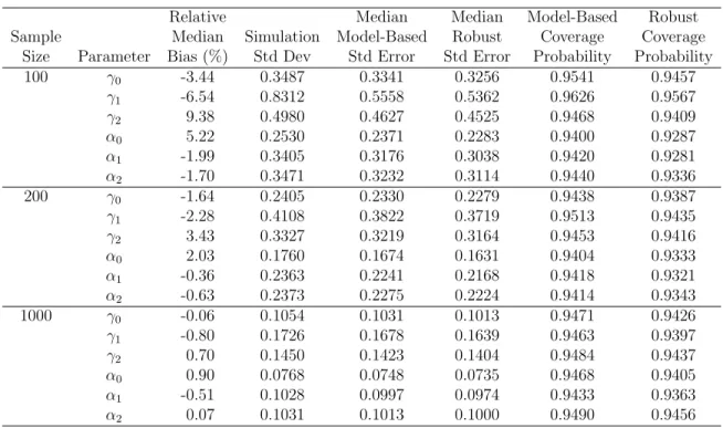
From Table 2.1, we note that the marginalized ZIP has low bias for αand the bias generally decreases with increasing sample size. For most parameters, the model-based standard errors are similar to the standard deviation of the simulated parameter esti-mates, implying adequate estimation of the standard error of the parameter estimates. For all sample sizes, Wald-type confidence intervals of the marginalized ZIP param-eters have model-based coverage probabilities near the expected 0.95, and coverage probabilities created using the robust standard error have fractionally less coverage.

Additionally, a simulation study was performed to compare the new marginalized ZIP model to several existing methods, namely the traditional ZIP model employing a delta method transformation for post-hoc estimation of overall effects due to xi1. We also used Poisson regression to model each simulated data set and obtain estimates of IDR, both with and without deviance scaling for overdispersion. Since Preisser et al. (2012) found that many researchers interpreted the ZIP latent class parameters as population-level parameters, we examined the properties of these na¨ıve ZIP interpre-tations as well.

For the traditional ZIP, the relationship between the parameter estimates and the IDR is

E(Yi|xi1 = 1, x2)

E(Yi|xi1 = 0, x2)

=eβ1 1 + exp(γ0+γ2xi2) 1 + exp(γ0+γ1+γ2xi2)

. (2.6)

Note that this relationship produces multiple IDR’s, one for each value of the extraneous covariatexi2. For these simulations, ¯x2 = _n1Pn_i₌₁xi2 was used to calculate the log-IDR and its standard error for the traditional ZIP model and delta method. However, this IDR estimate represents the IDR for an ‘average’ individual, potentially unobservable in the sample population. The use of the na¨ıve ZIP parameter interpretations would presenteβ1 _{as the IDR, failing to recognize the relationship between IDR and the} zero-inflated parametersγ. Using data generation as described above, the marginalized ZIP

(38)

and traditional ZIP were both performed, then the delta method transformation was used to obtain the latter’s estimates of the log-IDR and standard error of log-IDR. Additionally, 95% Wald-type confidence intervals for the log-IDR were created using the point estimate and respective standard error. For each of the methods described, Table 2.2 presents the relative median bias in estimating the IDR and log-IDR, Table 2.3 presents coverage probabilities and Table 2.4 displays power. For the marginalized ZIP and Poisson regression models, robust estimators of the covariance matrix were also employed to calculate the 95% Wald-type confidence intervals, as well as their corresponding coverage probabilities and power. Results are presented for varying levels of the true incidence density ratio eα1_{, where} {_γ

0 = 0.60, α0 =−0.25, γ1 = −1,

α1 ={log(1.25),log(1.5),log(2)},γ2 =α2 = 0.25}.

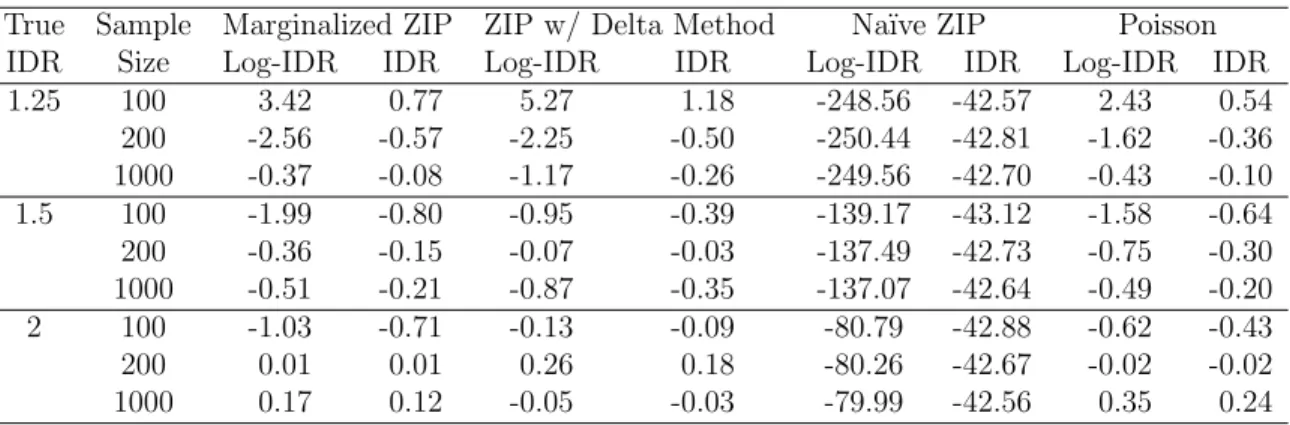
With regards to bias, Table 2.2 shows that the marginalized ZIP, ZIP with delta method transformation and Poisson regression models all have low relative bias in estimating both the log-IDR and IDR. However, the na¨ıve ZIP parameter interpretation yields very biased estimates for both log-IDR and IDR. For the fixed parameter values and (2.6), we can determine the expected relative bias in IDR under the na¨ıve ZIP model to be

Percent Relative Bias = e

β1 ₋_eα1

eα1 ×100

= 1− 1 + exp(γ0+γ1+γ2x¯i2) 1 + exp(γ0+γ2x¯i2)

×100

= 42.24

regardless of true IDR. This quantity is driven by the magnitude of the exposure pa-rameter in the zero-inflated process.

(39)

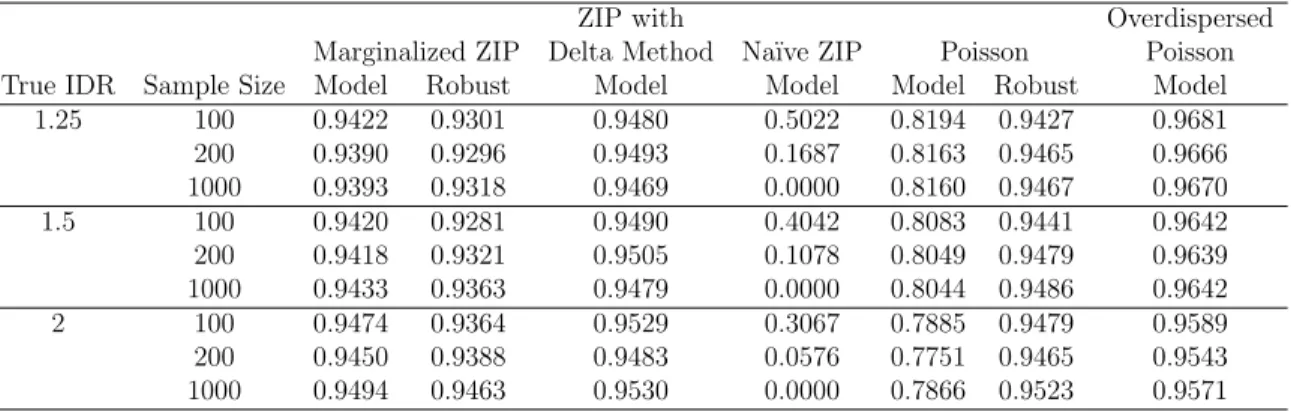
each method described. Again, since the na¨ıve ZIP parameter interpretation is esti-mating the wrong quantity, the coverage of the true IDR goes to zero as the sample size increases. The marginalized ZIP, ZIP with delta method transformation, Poisson with robust variance estimator and overdispersed Poisson models all have appropriate coverage, with the Poisson with model-based variance estimator having less coverage than desirable.

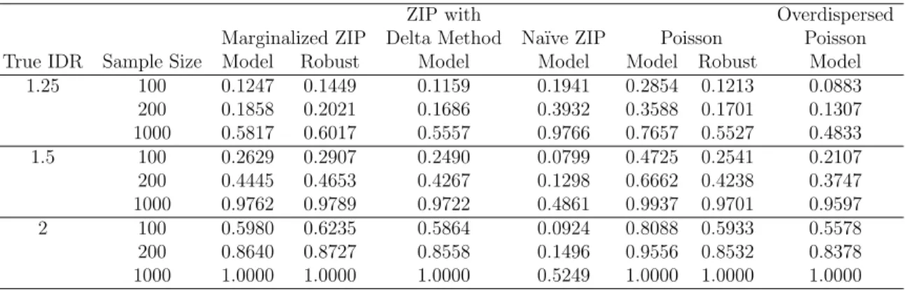
Examining the power from each method, the marginalized ZIP has slightly more power than the ZIP with delta method transformation, Poisson with robust variance estimate and overdispersed Poisson under nearly every scenario. For a given sample size, we observed a non-monotone relationship between power and true IDR for the na¨ıve ZIP interpretation. This phenomenon is a result of rejections of the null hypothesis with estimated IDR below 1 when the true IDR is 1.25. For large sample sizes, this na¨ıve interpretation has high power to detect an incorrect IDR, emphasizing the need for direct methods to achieve marginal interpretations.

2.5 Motivational Interviewing Intervention Example

Reducing risky sexual behavior among people living with HIV/AIDS is one area of focus among infectious disease researchers, and one measure of risky behavior is the UAVI count, the number of Unprotected Anal or Vaginal sexual Intercourse acts within a given time period. The SafeTalk program was developed as a motivational interviewing-based intervention to reduce sexual behavior, particularly UAVI (Golin et al., 2010). To assess SafeTalk’s efficacy at reducing unprotected sex acts in this population, a randomized clinical trial was performed with subjects recruited at three sites being randomized to receive either SafeTalk or a nutritional intervention as control. The participants were then surveyed every four months for one year to measure their self-reported sexual acts in the previous three-month period. Since the primary research

(40)

question for this study is whether those in the SafeTalk intervention have lower UAVI than those in the control at the eight-month follow-up visit, the marginalized ZIP is employed to quantify the effect of treatment on UAVI.

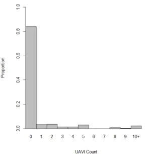
For this analysis, there are 357 participants with non-missing UAVI counts at the 8-month visit, excluding eight participants with UAVI counts greater than 18. Figure 2.1 shows the distribution of UAVI counts, which contains 300 (84%) zeros and 8 ‘10+’ counts (2.2%). Since the randomization scheme stratified by site, the marginalized ZIP model to be fit is

logit(ψi) = γ0+γ1xi1+γ2xi2+γ3xi3+γ4xi4

log(νi) = α0+α1xi1+α2xi2 +α3xi3+α4xi4

wherexi1 is an indicator of whether the ith participant received the SafeTalk interven-tion and xi2 and xi3 are indicators of whether the ith participant was randomized at the second and third study sites, respectively. Additionally, the analysis controls for baseline UAVI countxi4.

In order to compare the traditional ZIP model fit to the marginalized ZIP model, the standardized Pearson residuals of each method were computed and plotted in Figure (2.2). We investigated potential outliers in this manner, finally electing to remove all observations with UAVI greater than 18.

(41)

Sites 1, 2 and 3, the IDR (and corresponding 95% confidence intervals) from the trans-formed ZIP with fixed mean baseline UAVI count are 1.2360 (0.706, 2.165), 1.2399 (0.704, 2.184), and 1.2429 (0.701, 2.203), respectively. Examining the range of IDR across baseline UAVI counts, the IDR and corresponding 95% confidence intervals for zero and 18 baseline UAVI counts are 1.2487 (0.702, 2.222) and 0.9598 (0.727, 1.267). For this particular example, there does not appear to be much difference in the IDR of treatment across sites, but note the moderate change in IDR estimates for the different baseline UAVI counts. Although none of these estimates are statistically significant, the estimates for different combinations of covariates demonstrate the lack of a single IDR measure when using traditional ZIP with the delta method. In fact, particular transformed ZIP analyses may yield very different IDR estimates for various combina-tions of covariate values. Also, notice the transformed ZIP methods require significantly more effort and expertise in deriving and programming than the direct estimation of the log-IDR through the marginalized ZIP model.

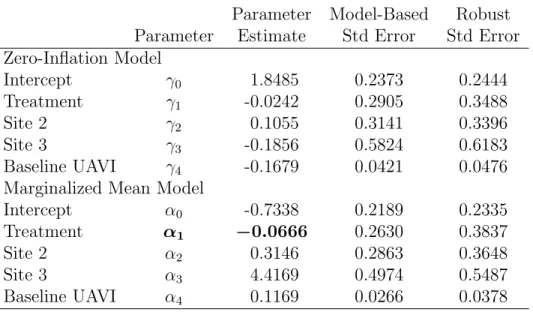
Table 2.5 presents the results of the marginalized ZIP analysis on the SafeTalk ex-ample. By exponentiatingα1, the estimate of the IDR for treatment is exp(−0.0666) = 0.9355; thus, the marginalized ZIP model reveals those on SafeTalk intervention have 6% fewer unprotected sexual acts at the eight-month followup visit than those partici-pants randomized to control. The 95% model-based Wald-type confidence interval for the treatment IDR is (0.559,1.567), implying there is no significant difference between the two treatment groups. However, this illustrative analysis is not considered defini-tive due to the deletion of large UAVI counts. Because the traditional ZIP with delta method is limited by the substitution of specific levels of the extraneous covariates, the overall effect of SafeTalk is difficult to summarize briefly. However, the marginalized ZIP model gives one IDR of SafeTalk intervention, adjusted for all the other covariates. In terms of model fit, the full likelihood values for the marginalized ZIP and traditional

(42)

ZIP models are -291.28 and -288.51, indicating that the two models have similar fit to the SafeTalk data.

2.6 Conclusion

In this manuscript, we develop a new marginalized ZIP model to achieve population-average estimates rather than the traditional ZIP latent class estimates, whose interpre-tations are difficult to convey. The primary advantage of the marginalized ZIP model is the direct estimation of the population mean, offering meaningful statements about an exposure effect on an entire sampled population rather than an unobservable latent class. Thus, arguably the marginalized ZIP model yields more interpretable results than the traditional ZIP model, for which additional calculations, involving more time and statistical expertise, are required to achieve population-level inference. Particularly, exposure effect estimation in the presence of covariates requires no additional assump-tions or estimation. Not only does the marginalized ZIP have relatively low bias, but it also outperforms traditional ZIP in estimating overall exposure effect estimates in power in a simulation study.

(43)

Figure 2.1: Histogram of UAVI Counts

(44)

(45)

Table 2.1: Marginalized ZIP Performance with 10,000 Simulations and Varying Sample Size

Relative Median Median Model-Based Robust Sample Median Simulation Model-Based Robust Coverage Coverage

Size Parameter Bias (%) Std Dev Std Error Std Error Probability Probability

100 γ0 -3.44 0.3487 0.3341 0.3256 0.9541 0.9457

γ1 -6.54 0.8312 0.5558 0.5362 0.9626 0.9567

γ2 9.38 0.4980 0.4627 0.4525 0.9468 0.9409

α0 5.22 0.2530 0.2371 0.2283 0.9400 0.9287

α1 -1.99 0.3405 0.3176 0.3038 0.9420 0.9281

α2 -1.70 0.3471 0.3232 0.3114 0.9440 0.9336

200 γ0 -1.64 0.2405 0.2330 0.2279 0.9438 0.9387

γ1 -2.28 0.4108 0.3822 0.3719 0.9513 0.9435

γ2 3.43 0.3327 0.3219 0.3164 0.9453 0.9416

α0 2.03 0.1760 0.1674 0.1631 0.9404 0.9333

α1 -0.36 0.2363 0.2241 0.2168 0.9418 0.9321

α2 -0.63 0.2373 0.2275 0.2224 0.9414 0.9343

1000 γ0 -0.06 0.1054 0.1031 0.1013 0.9471 0.9426

γ1 -0.80 0.1726 0.1678 0.1639 0.9463 0.9397

γ2 0.70 0.1450 0.1423 0.1404 0.9484 0.9437

α0 0.90 0.0768 0.0748 0.0735 0.9468 0.9405

α1 -0.51 0.1028 0.0997 0.0974 0.9433 0.9363

α2 0.07 0.1031 0.1013 0.1000 0.9490 0.9456

(46)

Table 2.2: Comparison of Relative Median Biases for Estimation of Overall Exposure Effects with Marginalized ZIP, ZIP with Delta Transformation, ZIP with Na¨ıve Inter-pretations, & Poisson

(47)

Table 2.3: Comparison of Coverage Probabilities for Estimation of Overall Exposure Effects with Marginalized ZIP, ZIP with Delta Transformation, ZIP with Na¨ıve Inter-pretations, & Poisson

ZIP with Overdispersed

Marginalized ZIP Delta Method Na¨ıve ZIP Poisson Poisson

True IDR Sample Size Model Robust Model Model Model Robust Model

1.25 100 0.9422 0.9301 0.9480 0.5022 0.8194 0.9427 0.9681

200 0.9390 0.9296 0.9493 0.1687 0.8163 0.9465 0.9666

1000 0.9393 0.9318 0.9469 0.0000 0.8160 0.9467 0.9670

1.5 100 0.9420 0.9281 0.9490 0.4042 0.8083 0.9441 0.9642

200 0.9418 0.9321 0.9505 0.1078 0.8049 0.9479 0.9639

1000 0.9433 0.9363 0.9479 0.0000 0.8044 0.9486 0.9642

2 100 0.9474 0.9364 0.9529 0.3067 0.7885 0.9479 0.9589

200 0.9450 0.9388 0.9483 0.0576 0.7751 0.9465 0.9543

1000 0.9494 0.9463 0.9530 0.0000 0.7866 0.9523 0.9571

(48)

Table 2.4: Comparison of Power for Estimation of Overall Exposure Effects with Marginalized ZIP, ZIP with Delta Transformation, ZIP with Na¨ıve Interpretations, & Poisson

ZIP with Overdispersed

Marginalized ZIP Delta Method Na¨ıve ZIP Poisson Poisson

True IDR Sample Size Model Robust Model Model Model Robust Model

1.25 100 0.1247 0.1449 0.1159 0.1941 0.2854 0.1213 0.0883

200 0.1858 0.2021 0.1686 0.3932 0.3588 0.1701 0.1307

1000 0.5817 0.6017 0.5557 0.9766 0.7657 0.5527 0.4833

1.5 100 0.2629 0.2907 0.2490 0.0799 0.4725 0.2541 0.2107

200 0.4445 0.4653 0.4267 0.1298 0.6662 0.4238 0.3747

1000 0.9762 0.9789 0.9722 0.4861 0.9937 0.9701 0.9597

2 100 0.5980 0.6235 0.5864 0.0924 0.8088 0.5933 0.5578

200 0.8640 0.8727 0.8558 0.1496 0.9556 0.8532 0.8378

(49)

Table 2.5: Marginalized ZIP Model Results: SafeTalk Example

Parameter Model-Based Robust Parameter Estimate Std Error Std Error Zero-Inflation Model

Intercept γ0 1.8485 0.2373 0.2444

Treatment γ1 -0.0242 0.2905 0.3488

Site 2 γ2 0.1055 0.3141 0.3396

Site 3 γ3 -0.1856 0.5824 0.6183

Baseline UAVI γ4 -0.1679 0.0421 0.0476 Marginalized Mean Model

Intercept α0 -0.7338 0.2189 0.2335

Treatment α1 −0.0666 0.2630 0.3837

Site 2 α2 0.3146 0.2863 0.3648

Site 3 α3 4.4169 0.4974 0.5487

Baseline UAVI α4 0.1169 0.0266 0.0378

(50)

Chapter 3 Marginalized ZIP Regression Model

with Random Effects

3.1 Introduction

Infectious disease researchers are often concerned with reducing risky sexual be-havior among HIV-positive individuals. One measure of risky sexual bebe-havior is the Unprotected Anal and Vaginal Intercourse (UAVI) count, the number of unprotected anal or vaginal intercourse acts with any partner over a specified period of time. The SafeTalk program was developed by Golin et al. (2010) to reduce the number of unpro-tected sexual acts through a multicomponent, motivational interviewing-based, safer sex intervention. Sexual behavior count data can display a distribution with excess zeros (Heilbron, 1994; Ghosh and Tu, 2009). To examine the efficacy of the SafeTalk program over time, a randomized controlled clinical trial collected risky sexual behavior data at baseline and up to three follow-up visits.

(51)

In order to account for overdispersion beyond the excess zeros, Yau, Wang and Lee (2003) modify the zero-inflated negative-binomial (ZINB) regression model to include random effects. Instead of using random effects to handle correlated data, Hall and Zhang (2004) employ GEE methodology for zero-inflated models in order to achieve population-averaged interpretations. For each of these zero-inflated methods, two sets of parameter estimates are produced, those associated with the excess zero process and those associated with the count process. Although many health-related fields are implementing zero-inflated techniques, these two sets of parameter estimates can be difficult to interpret, in many cases leading to incorrect statements (Preisser, et al., 2012). Often health researchers wish to make inference upon an entire sampled population rather than the latent classes modeled by ZIP methodology. Transformation methods, with variance estimation by the delta method or resampling methods, may be used to make inference on overall estimates of exposure effect for ZIP and ZINB models (Albert, et al., 2011). However, such transformations can be tedious for many analysts, and the treatment of covariates is not necessarily apparent.

While closely related to the zero-inflated methodology, hurdle models (including zero-altered models) account for excess zeros by modeling all zeros separately from positive counts (Mullahy, 1986; Heilbron, 1994). One set of parameters measures effects on the probability of being a zero and one set measures effects on the mean conditional on the observation being positive. Dobbie and Welsh (2001) use the zero-altered Poisson model, modified to utilize GEE, to account for correlated observations. Min and Agresti (2005) extend the zero-altered model to include random effects. Like ZIP models, hurdle models do not produce a direct overall estimate of exposure effect for the marginal mean count.

The choice between the hurdle and zero-inflated model classes has been approached from various angles. Much of the literature pertaining to the analysis of count data

(52)

with excess zeros focuses on model fit, using fit statistics to provide justification of model class choice. Gilthorpe, et al. (2009) argue that a priori knowledge of the data-generating mechanism could be used to identify the class of models from which to choose, supported by statements in Neelon et al. (2010) and Buu et al. (2012). Applications in which all zeros can be considered as arising from an identical process indicate a hurdle model, rather than a zero-inflated model, where zeros can occur from the two different processes. Albert et al. (2009) contend that model interpretations have been generally overlooked in the zero-inflated literature; they propose methods for the assessment of overall exposure effects. In many applications containing count data with many zeros, the two latent class interpretations are not clinically supported, and the zero-inflated methodology is just a modeling technique to account for excess zeros in a single population (Mwalili, et al., 2008).

Proposing the marginalized model for longitudinal binary data, Heagerty (1999) employs joint models by directly modeling the marginal mean and simultaneously us-ing a linked random effects model to account for correlated responses. Through this joint model, marginalization over random effects achieves population-averaged param-eters, while accounting for correlated measures. Extending the marginalized model approach, Lee et al. (2011) focus on the hurdle model formulation for Poisson and negative binomial data with excess zeros while marginalizing over random effects for clustering. Since Lee et al. focus on marginalizing over the random effects, the two sets of parameters from their marginalized hurdle models have the same interpretations as hurdle models for independent responses.

(53)

the marginalized ZIP model with random effects, which has subject-specific parameters and discuss the situation where those parameters have equivalent population-averaged interpretations. Section 4 presents simulation study results examining the finite sample performance of the new model. In Section 5, we consider data from the SafeTalk randomized controlled clinical trial. A discussion is provided in Section 6.

3.2 ZIP Model with Random Effects

Extending Lambert’s ZIP model to incorporate correlated zero-inflated count data, Hall (2000) developed the ZIP model with random effects. Let Y = (Y₁0, . . . ,Y_K0) where K is the number of independent clusters and Yi = (Yi1, . . . , YiTi)

0_{, where} _T

i is

the number of observations for theith _{cluster. Let}_s

ij = 1 ifYij is from the first process

(i.e. Yij is an excess zero) andsij = 2 ifYij is from the second (Poisson) process. Then

Yij ∼

      

0 with probability P(sij = 1) =ψij

Poisson (µC

ij) with probability P(sij = 2) = 1−P(sij = 1) = 1−ψij

(3.1)

where µC_ij = E(Yij|sij = 2, bi). The notation µCij indicates that the Poisson mean is

conditional on the random effect bi. The log-linear and logistic regression models are

logit(ψij) = Zij0 γ

log(µC_ij) = X_ij0 β+σbi,

whereb1, . . . , bK i.i.d.

∼ N(0,1), and Zij andXij are the covariate vectors for the logistic

and Poisson processes, respectively. The log-likelihood can be expressed

l(θ,y) =

K X i=1 log Z ∞ −∞ " _T i Y j=1

Pr(Yij =yij|bi)

#

φ(bi) dbi

(54)

whereθ = (γ0,β0, σ), φ is the standard normal probability density and

Pr(Yij =yij|bi,θ) =

h

ψij + (1−ψij)e−µ

C ij

iuij

"

(1−ψij)e−µ

C ij(µC

ij)yij

yij!

#1−uij (3.2)

= (1 +eZij0 γ₎−1

(

uij

h

eZij0 γ + exp(−_eXij0 β+σbi₎i + (1−uij)

exp[yij(Xij0 β+σbi)−eX

0

ijβ+σbi_]

yij!

)

,

where uij = I(yij = 0). Using the EM algorithm framework that Lambert (1992)

proposed, Hall fits this ZIP model with random effects with the EM algorithm with Gaussian quadrature. Generally, the overall conditional mean E(Yij|bi) = (1−ψij)µCij

will depend on γ, β and bi through a complicated function that does not permit easy

and direct inference for overall effects, here defined as ratios of such means when a single covariate is allowed to vary.

3.3 Marginalized ZIP Model with Random Effects

3.3.1 Subject-specific marginalized ZIP model

Using a marginalized model approach, we now present a marginalized adaptation of the ZIP model with random effects for repeated measures data. The marginalized ZIP model for clustered data directly models the overall subject-specific mean ν_ijC =

E(Yij|di) through

logit(ψ_ijC) = Z_ij0 γ+w0₁_ijci

(55)

whereψC_ij =P(sij = 1|ci) andbi = (ci,di)0 follows the multivariate normal distribution

with mean zero and covariance matrix Σ =

  

Σ11 Σ12 Σ21 Σ22

 

. Because ν

C

ij is modeled

directly in this marginalized ZIP with random effects model, αk is interpreted as the

subject-specific log-incidence density ratio (IDR) for the kth _{covariate; that is, for a}

one-unit increase in corresponding covariate xk, exp(αk) is the amount by which the

meanν_ijC for a particular subject is multiplied, which is the same interpretation as in a Poisson random effects model.

Forθ = (γ0,α0,Σ)0, the log-likelihood for this marginalized ZIP model with random effects can be written

l(θ;y) =

K

X

i=1 log

Z +∞

−∞

" _T_i Y

j=1

P(Yij =yij|bi,θ)

#

Φ(bi)dbi, (3.4)

where Φ is the multivariate normal density (0,Σ). In order to use the ZIP likelihood presented in (3.2), we redefine µC

ij = exp(δCij), where δCij is not necessarily a linear

function of covariates. Then

P(Yij =yij|bi,θ) =

h

ψC_ij + (1−ψC_ij)e−exp(δCij)

iI(yij=0) "

(1−ψC ij)e

−exp(δC ij)eδCijyij

yij!

#I(yij>0) (3.5)

Substitution of (3.3) into νC

ij = (1−ψijC)µijC and solving for δijC = log(µCij) gives

δC_ij = log(Ni) + log[1 + exp(Zij0 γ+w

0

1ijci)] +Xij0 α+w

0

2ijdi. (3.6)

Through substitution of (3.6) into (3.5), this subject-specific marginalized ZIP model with random effects may be fit using SAS NLMIXED (SAS Institute Inc, 2013), which employs an adaptive Gauss-Hermite quadrature to approximate the integral of the likelihood (3.4) over the random effects. Also, SAS NLMIXED can provide robust

(56)

(empirical) standard error estimates of the parameters, through the likelihood-based ‘sandwich’ estimator, to address model misspecification (White, 1982).

3.3.2 Population-averaged marginalized ZIP model for

clus-tered data

The primary objective in the marginalized models literature (e.g. Heagerty, 1999) is to obtain marginalized (or population-averaged) parameters rather than subject-specific parameters. In Section 3.3.1, we described the marginalized ZIP model with random effects, where the ‘marginalization’ is over the two latent classes of the ZIP model to achieve overall exposure effect estimates. However, because the marginalized ZIP with random effects models νC

ij =E(Yij|di), it yields parameters with subject-specific

interpretations.

For data with repeated measures, statistical analysts usually choose between meth-ods employing subject-specific (SS) parameters (mixed models) and methmeth-ods having population-average (PA) parameters (GEE). However, Ritz and Spiegelman (2004) and Young et al. (2007) investigate the exact nature of the relationship between SS and PA parameters for Poisson count data, using methods established in McCulloch and Searle (2001). For models with log links and normally distributed random effects, the math-ematical relationships between SS and PA parameters can be quite straightforward.

To explore the connection between SS and PA parameters for the marginalized ZIP model with random effects, we restate the model as

logit(ψ_ijC) = Z_ij0 γSS+w0₁_ijci

log (ν_ijC) = X_ij0 αSS+ log(Ni) +w02ijdi, (3.7)

(57)

for these parameters. Then

E(Yij|di) = exp[Xi0α

SS_{+ log(}_N

i) +w20ijdi]

and

E(Yij) = E[E(Yij|di)] (3.8)

= Niexp(Xi0α SS

)E(exp(w0₂_ijdi))

= Niexp(Xi0α

SS_{) exp(0}_.₅_w0

2ijΣ22w2ij)

wheredi ∼N(0,Σ22). From (3.8), defining νijM =E(Yij),

log(ν_ijM) = X_ij0 αSS + log(Ni) + 0.5w02ijΣ22w2ij. (3.9)

Now consider the fully marginal model (3.10), where P A denotes population-averaged parameters

log(ν_ijM) = X_ij0 αP A+ log(Ni). (3.10)

The PA parameters in (3.10) are multiplicatively offset from the SS parameters by the function exp(0.5w₂0_ijΣ22w2ij) of the Poisson random effects and respective covariance

matrix. Thus, for all covariates that do not have corresponding random effects inw₂0_ij, the corresponding parameters αSS _{are equivalent to} _αP A_{. Consider the model with}

only a random intercept (w0₂_ij = 1) and Σ22=σb2; then

log(ν_ijM) = [αSS₀ + (σ_b2/2)] +X˜_i0α˜SS+ log(Ni),

where ˜X_i0 and α˜SS _{contain all the covariates and corresponding parameters excluding}

(58)

the intercept. In this situation, α˜SS also have population-averaged interpretations. While analysts may choose to include further normal random effects, such as a random slope over time, all parameters without a corresponding random effect have population-averaged as well as subject-specific interpretations because of the log link and normal random effects.

3.4 Simulation Study

To examine the properties of the marginalized ZIP model with random effects, a simulation study was performed using SAS 9.3 NLMIXED. Let Yij be a zero-inflated

Poisson outcome for theith_{participant at time}_j_{, and let}_g

i be a time-constant exposure

variable of interest for each subject. The simulation scenario is motivated by the constant treatment assignment in the SafeTalk clinical trial. In the SafeTalk motivating example,Yij is the UAVI count outcome andgi is an indicator of randomization to the

SafeTalk intervention group. For this simulation study, three time points were used with I(j = 2) and I(j = 3) being the indicators of whether an observation occurs at follow-up time 2 or 3. Data were simulated using the marginalized ZIP model with random effects given by

logit(ψ_ijC) = γ0+γ1I(j = 2) +γ2I(j = 2)gi+γ3I(j = 3) +γ4I(j = 3)gi+ci

log(ν_ijC) = α0+α1I(j = 2) +α2I(j = 2)gi+α3I(j = 3) +α4I(j = 3)gi +(3.11)di,

where ci, di are independent normal random intercepts with variances σ12 and σ22 used to account for correlated outcomes for the ith _{participant. Although we designed the}