MANIPULATION OF SINGLE DNA MOLECULES THROUGH NANO-FLUDIC DEVICES: SIMULATION AND THEORY
Yanqian Wang
A dissertation submitted to the faculty at the University of North Carolina at Chapel Hill in partial fulfillment of the requirements for the degree of Doctor of Philosophy in the Department of Physics.
Chapel Hill 2016
Approved by: Adam R. Hall Jack Ng
ABSTRACT
Yanqian Wang: Manipulation of Single DNA Molecules through Nano-fludic Devices: Simulation and Theory
(Under the direction of Michael Rubinstein)
Nanofludic platforms such as solid-state nanopores and nanochannels enable the manipulation of DNA molecules and have the potential to be a low-cost and high-efficiency DNA sequencing device.
DNA nanopore translocation is a process where DNA moves from one chamber to another through a nanopore. To get into the pore, the molecule entropy decreases and free energy increases. In order to thread the DNA throughout the pore, an electric bias is applied to overcome the entropic energy barrier. The occupation of DNA impedes the ion transport and creates a blockage current of which the amplitude and duration provide the information on the DNA sequence since different bases (or base pairs) can be discriminated through different magnitude of blockage. Mining DNA sequence from the electric current profile requires an accurate knowledge of the passage time of a given base along the molecule. Our model assumes that the translocation process at high fields proceeds too fast for the chain to relax, and thus the distribution of translocation times of a given monomer are controlled by the initial conformation of the chain (the distribution of its loops). The model predicts the translocation time distribution is determined by the distribution of initial conformation as well as by the thermal fluctuations to the conformation during the translocation process.
TABLE OF CONTENTS
LIST OF FIGURES . . . vii
LIST OF ABBREVIATIONS AND SYMBOLS . . . viii
1 Introduction . . . 1
1.1 DNA manipulation and sequencing . . . 1
1.2 Nanopore DNA sequencing . . . 3
1.2.1 Protein nanopores . . . 3
1.2.2 Solid-state nanopores . . . 4
2 DNA translocation through nanopores. . . 8
2.1 Introduction . . . 9
2.2 Model description . . . 11
2.2.1 Brownian motion . . . 13
2.2.2 Translocation time . . . 20
2.2.3 Thermal fluctuations . . . 21
2.2.4 Conformational fluctuation . . . 23
2.3 Simulation setup . . . 23
2.4 Results and discussion . . . 25
2.5 Concluding remarks . . . 27
2.6 Figures . . . 28
3 Single ds-DNA molecules in nanochannels . . . 34
3.1 Introduction . . . 34
3.3 Single DNA molecules confined to a nanochannel . . . 36
3.4 Compressed DNA molecule in a nanochannel . . . 37
3.5 Electrohydrodynamic force on DNA molecule in a nanochannel . . . 38
3.5.1 Electrophoresis of microgel in bulk solution . . . 39
3.5.2 Immobile microgel in bulk solution . . . 39
3.5.3 Derivation of the electro-hydrodynamic force on semiflexible polyelectrolytes in nanochannels . . . 40
3.5.4 A compressed DNA molecule in a nanochannel . . . 47
3.6 Figures . . . 50
4 Enhanced nanochannel translocation and localization of genomic DNA molecules using three-dimensional nanofunnels . . . 53
4.1 Introduction . . . 53
4.1.1 Funnel shapes . . . 53
4.2 Models . . . 55
4.2.1 Confinement force . . . 55
4.2.2 Elastic force . . . 56
4.2.3 Electrohydrodynamic force . . . 57
4.2.4 Osmotic gradient force . . . 60
4.2.5 Effective free energy barrier . . . 60
4.2.6 Thermal fluctuations . . . 61
4.3 Results . . . 65
4.3.1 Comparison of theoretical and experimental values . . . 65
4.3.2 Lowering threshold electric field using nanofunnels . . . 66
4.3.3 Trapping of DNA using electro-osmotic tweezers . . . 67
4.4 Figures . . . 70
LIST OF FIGURES
2.1 A cartoon illustration of the theoretical model of forced translocation. . . 28 2.2 The setup of 3D Langevin Dynamics simulation of translocation. . . 29 2.3 The traces of the translocation times from two chains with distinct initial conformations. . . 30 2.4 The ensemble averaged translocation time. . . 31 2.5 Comparison of the thermal broadening to the conformational broadening of
translo-cation times. . . 32 2.6 Comparing the simulation results of conformational broadening with the model’s prediction. . 33
3.1 Regimes of the conformations of free semiflexible polymers in nanochannel confinement. . . . 50 3.2 Conformation of a single molecule in a nanochannel. . . 51 3.3 Flow profile within and around the molecules. . . 52
4.1 Comparison of DNA threading into a nanochannel directly or through a
three-dimensional nanofunnel. . . 70 4.2 Comparison of DNA threading into a nanochannel directly or through a
three-dimensional nanofunnel. . . 71 4.3 Comparison of experimental and theoretical x0,xN distributions for trapping of
T4-phage DNA. . . 72 4.4 Electric field dependent average positions and fluctuations ofλ-phage DNA molecules
trapped in a three-dimensional (α=0.45) nanofunnel. . . 73 4.5 Electric field dependent average positions and fluctuations of T4 -phage DNA
LIST OF ABBREVIATIONS AND SYMBOLS
a diameter(width) of a polymer backbone AFM atomic force microscopy
b Khun length
bp basepair
c concentration of monomers cs salt concentration
ds- double-stranded DNA deoxyribonucleic acid e elementary charge E electric field
Et threshold electric field
DL Debye Layer EOF electro-osmotic flow fconf confinement gradient force
fdrag hydrodynamic drag force
feh electrohydrodynamic force
fel electrostatic force
felas elastic force
fosm osmotic gradient force
fstall stall force
F free energy
Fconf conformational part of the chain free energy
Fent entropic part of the chain free energy
Fint interaction part of the chain free energy
gT number of monomers in a thermal blob
kB Boltzmann’s constant
lB Bjerrum length
lp persistence length
L size of a polymer
Lchannel length of the nanochannel
Lf unnel length of the nanofunnel
N degree of polymerization q charge per a Khun monomer
qef f effective charge per a Kuhn monomer
qred reduced charge per a Kuhn monomer
Q hydraulic flux
rD Debye screening length
Re end-to-end distance
Rg radius of gyration
R|| the longitude size of a polymer in a channel
ss- single-stranded
t time
T absolute temperature
TEM transmission electron microscopy
UNC University of North Carolina (at Chapel Hill) v excluded volume of a monomer
V electrostatic potential
w effective width of a rod-like monomer ∆F free energy barrier
LJ interaction parameter of the Lennard-Jones potential
η solution viscosity
µ electrophoretic mobility ζ friction coefficient
ξ correlation length of a semidilute polymer solution ξH hydrodynamic screening length
ξT thermal blob size
Π polymeric osmotic pressure τ chain relaxation time τRouse Rouse relaxation time
CHAPTER 1: Introduction
Section 1.1: DNA manipulation and sequencing
Accurate genome sequencing is the key to deciphering the secrets of life and is vital for both fundamental research and medical diagnostics. In the past few decades, researchers have been eagerly developing and im-proving sequencing technologies. In 1977, Frederick Sanger and colleagues[104] proposed a DNA sequencing method based on chain-terminating dideoxynucleotides by polymerase and analyze each piece of dideoxynu-cleotides. During sequencing, the target DNA molecule is cut at known sites into fragments and separated using gel electrophoresis. By measuring the length of these DNA fragments and overlapping them with the aid of a computational algorithm, genomic information can be constructed. The Sanger method was the basis of the 13-year Human Genome Project[72], and demonstrated great accuracy and has been widely used since then.
Although the Sanger method is the most accurate DNA sequencing technique available today, it suffers from several limitations, which result in its high cost and long processing times. For example, applying gel electrophoresis to measure the lengths of DNA fragments requires large quantities of samples, which means that time-consuming and expensive cell cultures must be performed to provide sufficient quantities of cells. In some cases, not all species of cells can be cultured, which prevents the Sanger method from being used to sequence these species genomes. Even if the target cell culture is available, the genome of those replicated cells may not be exactly the same as the original culture due to genomic instability, genetic heterogeneity, and laboratory selection of genotype. The second issue with the Sanger method is that the measurement of DNA fragment lengths is on an ensemble basis, which can average out heterogeneity that may have biological and clinical significance. The third issue is that efficiency in measuring these genome fragments can only be increased so much. The electrophoretic separation of DNA fragments is based on length-dependent reptation motion of DNA molecules in a gel or nanoarray. Increasing the electric field can potentially accelerate the process, but will stretch the molecule and fail to completely separate DNA fragments due to length-independent electrophoretic mobility. Once the sizes of the fragments are determined, a search for overlapping sequences of the fragments requires alignment with a pre-existing sequence of the genome. However, such sequence maps of the genome are often not known.
many of them involve the mechanical control of the molecules position and movement. The incorporation of the mechanical control of a single DNA molecule into the DNA sequencing platform can facilitate the sequencing[115, 92]. For example, there are several techniques used to mechanically manipulate DNA[13], including atomic force microscopy (AFM)[46], micropipettes[13], optical tweezers[26], and fixed force mag-netic tweezers[92]. These techniques can be divided into either fixed-position methods, such as AFM, mi-cropipettes, and optical traps, or fixed-force methods, like the magnetic trap technique.
Although these methods provide important information about DNA, there are advantages and drawbacks to all these techniques. For example, AFM can be used to image and stretch a single DNA molecule with high spatial positioning accuracy of up to 0.1 nm using a very stiff cantilever. However, AFM techniques generate more signal noise compared to other approaches. The micropipette technique is usually accomplished with a weaker cantilever to provide an additional mode of rotation compared to AFM manipulation. For both the optical and magnetic trapping methods, researchers tether a micron-sized bead to the free end of a DNA molecule. In an optical trap system, the bead is approximately 0.5µm in size and is controlled via a trapping laser, which creates forces as high as 100 pN. Compared to the optical trapping method of DNA, the magnetic tweezer method provides easy rotation of the molecule and its weak stiffness results in a constant force that depends on bead size. Besides these DNA manipulation techniques, researchers have also adopted flow field systems[13] to study the static properties of the DNA molecule, such as tension when the molecule is stretched.
raised great research interest in recent decades.
Section 1.2: Nanopore DNA sequencing
About two decades ago, a promising low-cost and high-throughput sequencing method was first introduced using a nanopore to perform single-molecule real-time sequencing. The nanopore is embedded into a thin membrane separating ionic buffer solution into two chambers - cis and trans. DNA molecules are initially placed in the cis chamber and an electric bias is applied across the membrane to drive the negatively charged DNA molecules to the trans side through the nanopore. During translocation, when the nanopore is partially occupied/blocked by a DNA strand, the resistance of the nanopore increases compared to its vacant state prior to and after translocation. Such a change in resistance can be monitored through the observation of ionic current passing through the nanopore under certain electric biases. In principle, the occupation of the nanopore with a different genomic base induces a distinct resistance. Therefore the passage of a molecule through the pore generates a temporal pattern of ionic current from which the DNA sequence can be read. The whole idea is to transform the spatial sequence of a DNA molecule into easily observed temporal signals, i.e. electric current traces . Although the invention of an orifice-based sensor appeared as early as the 1940s by Coulter[W.R. Hogg], in which the transport of blood cells through a pore allowed researchers to count and size the analytes, the leap of using a nanopore platform to sequence DNA did not occur until 1996, with the work of Kasianowiczet al.[43].
1.2.1: Protein nanopores
In the work of Kasianowicz et al.[43], the authors embed an α-hemolysin protein pore into a lipid bi-layer. They then introduce single-stranded poly(U) RNA homopolymers into the cis chamber and force the molecules to pass through the protein nanopore using an applied electric bias. In their study, Kasianowicz et al. observed three distinct current blockades. The blockade with the shortest dwell time was interpreted as the collision of RNA molecules with the nanopore orifice. The other two types of blockades corresponded to RNA translocation events featuring two different entry orientations ( i.e., entry with either the 3’ or 5” terminus of the RNA molecule). The authors observed that each passage event provided a trace of blockage current, which indicated at least three features of the translocation process, including dwell time, current levels, and rate of events. Translocation dwell time depends on molecules length and the events rate is linked to the concentration of the analytes. The levels of the current in principle can tell the sequence of the DNA/RNA molecule.
[3], who studied how the current signal changed for different RNA and DNA molecules. In their work, the purine poly(A) molecule resulted in deeper blockages of current compared to the poly-pyrimidine poly(C) and poly(U) molecules; an observation which could not otherwise be explained by its primary structure and therefore was attributed to its voluminous secondary structure . In addition, the authors demonstrated a clear two-level current pulse during the translocation of a block co-polymer made of bases C and A. Meller et al. [74] also showed the capability of the α-hemolysin nanopore in distinguishing homopolymers and heteropolymers composed of nucleobases dA and dC .
A recently commercialized version of a protein nanopore based genome sequencing device was recently realized with the development of the MinION from Oxford Nanopore Technology. This $1000 device shows improved sequencing accuracy and has gained the attention of many researchers since its debut in 2015. The MinION can read up to 98 kilobases in length, though the average length is about 1 or 2 kilobases, with accuracies of greater than 90% [60].
Although the MinION uses enzymes as regulators to control the speed of translocation to improve the resolution, the reading precision is fundamentally limited by the simultaneous contribution of many bases to the current signal. More sophisticated algorithms, such as the Hidden Markov Model, have been applied to alleviate such difficulties. When these algorithms are paired with alignment strategies, the read-out accuracy can be improved by up to 99% for some analytes [42], which is comparable to other real-time sequencing technologies, such as SMRT [22], though still well below the accuracy of the Sanger sequencing method, which has an overall accuracy on the order of 99.95% [60].
1.2.2: Solid-state nanopores
Although protebased nanopores have atomically precise dimensions and consistent pore-molecule in-teractions, they are also fragile given the imperfect stability of the lipid bilayer. The dimensions of protein nanopores are also not tunable, which is a drawback for experimental design.
As an alternative to protein nanopores, solid-state nanopores, such as those fabricated from silicon nitride (SiN) have also demonstrated the power to discriminate among different nucleic acid polymers[35]. In contrast, solid-state nanopores are more flexible in terms of dimension and shape, and they are robust under many different thermal and chemical conditions [58], unlike protein nanopore experiments.
membranes and nanopores tend to enable greater numbers of translocating bases to contribute to the current signal, which complicates and lowers the accuracy of the sequence read-out. Despite the unsatisfactory status quo of fabrication, solid-state nanopores are generally easier to fabricate into arrays for parallel analysis [120], and integrate with other electronic [85] and optical devices [73].
Since a thick membrane results in the occupation of multiple nucleobases inside the nanopore and thus their simultaneous contributions to the electrical current signal. This makes it difficult to identify bases from the current traces. The emergence of new membrane materials enables researchers to fabricate ultra-thin nanopores. For example, a nanopore fabricated on a graphene membrane can be as thin as 0.34 nm, which is comparable to the size of a single nucleotide and much smaller than the 12-nucleotides longβ-barrel region of aα-hemolysin nanopore [75]. Other promising substrates for nanopore fabrication include boron nitride (BN) and molybdenum disulfide (MoS2), the membranes of which can be just 1.1 nm [62] and 0.65 nm thick, respectively [61, 23].
Researchers have found that these kinds of ultra-thin nanopores have stronger interactions with DNA molecules, which is a double-edged sword[58]. Nanopores of thickness under 3 nm can slow the analytes translocation speed due to increased van der Walls interactions with the pore walls. Such intensified inter-actions can clog the pore and result in increased unreliability of the sequencing platform. Sometimes the material of the substrate itself can induce stronger interactions between the nanopore and analyte. For ex-ample, the slow translocation time of single-stranded DNA (ssDNA) through a graphene nanopore compared to a silicon nanopore of the same size is attributed to the hydrophobic adsorption of ssDNA to the graphene membrane [79, 38].
One large remaining challenge in solid-state nanopore sequencing is the rapidity of the translocation speed, which can be as fast as 30 base pairs(bp) per micro-second, faster than the allowed sequencing speed of around 1 bp per millisecond [58]. In general, a slower translocation speed can improve the temporal resolution of the read-out of the genome bases. Various strategies have been developed to slow down the translocation speed, such as by adding regulators to the DNA molecule[90] and changing the chemical/physical properties of the solvent and nanopore surface[15, 124, 114]. For example, lowering the temperature slows the motion of the ions and fluids, and also changes the DNA-nanopore interaction, leading to slower translocation speeds [119]. Researchers have also succeeded at elongating the translocation time by modulating the salt concentration and creating gradients between the cis and trans chambers[111, 118]. Decreasing the size of the counterions, K+>Na+>Li+, can also slow down DNA molecules due to a different mechanism of binding counterions to
DNA molecules[47].
the DNA and nanopore depends on the nanopore’s shape, size and material. Aksimentievet al. attributed the interaction to the hydrophobic adhesion between DNA and the nanopore walls [47]. In addition, cone-shaped nanopores can stretch double-stranded DNA (dsDNA) near the pore and facilitate the entry of the molecule due to the entropic interaction between the DNA and the nanopore [80]. In terms of material effects, researchers have observed that hafnium oxide (HfO2) nanopores slow DNA translocation by a factor of 10 compared to the same-sized nanopore made out of SiN [52]. Other nanopore membranes made of materials such as alumina oxide (Al2O3), BN, and graphene also slow translocation speeds by one order of magnitude in comparison to silicon counterparts [2, 62, 117]. Such slow-down was attributed to either the entropic, hydrophobic adhesion [4] or a contact friction [65] between DNA and the material inside nanopore wall.
The DNA and nanopore interaction is also tunable through modification of the nanopore’s surface charge. The surface charge affects translocation by changing the electroosmotic flow and the electrostatic interaction of DNA and the nanopore wall. For instance, the negative charge on SiN nanopore walls can be inverted to positive by coating the surface with a pH-sensitive polymeric cushion[5]. Although this method can change the surface charge density by a factor of 5 under feasible experimental conditions, it increases noise in the current signal due to a higher membrane capacitance.
Hydraulic pressure is another way to control the translocation speed of the DNA molecule by exerting a hydrodynamic force on the DNA in addition to the electric-field-induced force. By carefully adjusting the pressure, the translocation time can be prolonged by at least an order of magnitude[64]. The pressure-induced force is independent of the analytes charge, which allows this hydraulic pressure method to manipulate neutral polymers.
The interplay of hydraulic pressure and electric-fields can trap DNA in the nanopore and result in ultra-long translocation processes [37, 7, 125]. For the slow translocation events, the translocation dynamics are different from those in the ”fast” region of translocation events, for which non-equilibrium dynamics of the molecule apply. Slow translocation events allow the molecule to relax during the process. The first passage time analysis with Fokker-Planck equation can study the behavior in this regime[82, 83, 37]. One advantage of pressure modulated translocation over other methods, such as surface charge modification, is that it will not decrease the capture rate of the analyte or increase the noise of the current signal.
molecule. The magnitude of the electrical force can be obtained by measuring the displacement of the bead away from the focal point. In Keyseret al.’s experiments, dsDNA was found to have an effective charge of 0.5 e per base pair[44]. In their later experiments applying optical tweezers, the authors learned that the stall force increased with the decreasing nanopore size. Using this technique, they were able to reduce the translocation speed to 0.1 bp per millisecond, a reduction by 5 orders of magnitude[45].
Other mechanical control methods include magnetic tweezers, in which a magnetic field gradient is used to manipulate a DNA molecule that has been previously tethered to a magnetic-field-controlled bead[92]. However, the challenge of these mechanical strategies lies in the precise control of the bead. The Brownian motion of the bead and the molecule, especially when heated by a laser, decreases the resolution of the bead position, and at the same time increases the noise in the ionic current[58, 60, 108].
Besides slowing down the speed of translocation, researchers are developing new methods to better discriminate bases as they pass through the nanopore. One such method involves transverse electrodes, in which a pair of metal nanoelectrodes (such as freshly broken gold wires) are placed on the surface of the membrane at the location of the nanopore[127]. Zikic et al.[130] demonstrated that the tunneling current measured by the electrodes enabled the researchers to identify the four bases of ssDNA under different conditions of nanopore size and electric field strength [49, 50]. Another modification of this technology is to functionalize the transverse electrodes with different chemical reagents. When certain bases interact with the functionalized electrodes, they generate a transient tunneling current. The reagent can be customized to interact with different nucleotides. Since recognition is based on the transient current signal for each type of base, this method has the potential to realize sequencing under fast translocation speeds[39]. Other emerging methods to improve the distinguishability of bases includes the detection of current through nanogaps [94, 59] and graphene nanoribbon [79].
CHAPTER 2: DNA Translocation through Nanopores
Polymer translocation through a nanopore is encountered in a number of biological processes and re-searchers have considered it as a possible method to achieve rapid gene sequencing. However, the molecular details of this process and even the dependence of translocation time on the polymer chain length are not completely understood. In this dissertation, we determined the distribution of translocation times for a given monomer of the polymer chain using both analytical calculations and 3D Langevin dynamic simulations of forced translocation. A theoretical model of forced translocation of a polymer chain through a nanopore is proposed in this chapter. The model allows one to calculate the translocation time of individual monomers within a polymer chain featuring a particular initial conformation. The results of the computer simulation confirm the dependence of monomer translocation time on the polymer chain conformation. This chapter also studies, both analytically and numerically, the broadening of the distribution of translocation times due to the distribution of initial conformations and the thermal fluctuations of the polymer chain during the translocation process.1
1This chapter is adapted from a manuscript that is contributed by Yanqian Wang, Sergey Panyukov, Qi Liao and Michael
Section 2.1: Introduction
The nanopore platform has shown promise as a low-cost, high-throughput genome sequencing method. Kasianowiczet al.[43] pioneered early experiments that studied the translocation of biological macromolecules through a nanoscale pore. The authors specifically investigated the passage of single-stranded RNA and DNA molecules in an electric field through a narrow ion channel in a lipid bilayer membrane. They found that blockaded ion current could be used to detect the passage of DNA or RNA through the channel and ideally identify individual nucleotides. The duration of this current blockage time was found to increase with the degree of polymerization, as described in the relationshipτtrans∝N1.27, in whichτtrans is the translocation
time andN is the polymer chain length.
Many subsequent experiments adopted Kasianowiczet al.’s method and emphasized the influence of the strength of the external field on the translocation time and translocation velocity of a biomolecule through a channel. For example, Melleret al.[75] measured the velocity of single-stranded DNA translocation driven by an electric field through a single α-hemolysin pore. Their results verified that polymers longer than the pore length transported at a constant speed, while the translocation velocity of shorter polymers increased inversely with the chain length. The translocation velocity increased nonlinearly with increased applied voltage.
These initial studies on nanopore technology eventually led to the recently commercialized MinION Nanopore[78] released by Oxford Nanopore Technologies, which has been widely used in genome sequencing research and has the ability to read genome of up to 10 kilobases with a 90% accuracy rate per base[60]. However, such accuracy is still well below Sangers sequencing method. The Oxford Nanopore is made of a protein nanopore embeded in a lipid layer. The base recognition is limited by the simultanous contribution to the current signals by multiple bases inside of the constriction part of the protein nanopore. Although applying a more sophisticated algorithm [54] to analyze the raw data such as the Hidden Markov Model[42] can improve the readout accuracy, the fixed dimension of Oxford Nanopore puts a restriction on the tech-nology. Other researcher [56, 19, 79, 22, 105, 24, 32] seek to innovate the device itself. For instance solid state (SS) nanopore technology is more flexible in terms of dimensions and has the potential to enable single nucleotide read-out[112, 28, 60].
(Compared to voltage-driven DNA translocation, the enzyme regulated translocation allows the passage of genome bases one at a time and results in a higher sequencing accuracy. But the experimental condition is also largely limited in order to keep the enzyme active.) If the polymer enters the pore, it blocks the measured ion current, providing information about the translocation process. Storm et al.[56] studied translocation of double-stranded DNA through a silicon oxide nanopore and found a power-law scaling ofτtrans ∝N1.27,
which is different from the power-law relation obtained in many other results[27, 83]. Given the residence time as by far the most effective investigation tool for the translocation mechanism, different power-law relations of residence time will induce disparate or even conflicting fundamental understanding of the process. While studying polymer transolcation under a strong polymer-pore attraction, Krasilnikovet al.[48] observed that the residence time, the time duration that polymer occupies the nanopore, first increased and then decreased with molecular weight.
Besides experiments, a number of theoretical and simulation studies [40, 67, 29, 116, 10, 82, 9, 103, 55, 41, 27] has been devoted to the problem in the last decade. In the case of forced translocation, some researchers have claimed the dependence of τtrans ∝N2ν for short chains, and τtrans ∝ N1+ν for long chains in the
presence of an applied external field using a two-dimensional bond fluctuating model and two dimensional Langevin dynamics simulation, respectively [10, 40]. The Flory exponentν is 0.5 for ideal chain and 0.588 for swollen chain. Lubensky and Nelson [66] introduced a coarse-grained microscopic model to study the time distribution for polymers to pass through a pore when the chain has strong interactions with the pore itself. The authors claimed that translocation speed significantly depends on the polymers interaction within the pore and the interaction also increases the skewness of the distribution of the residence times.
In spite of notable progress, the problem of polymer translocation is far from being completely understood. In particular, there have been few studies on the origin of the variation of forced translocation time for a DNA/RNA chain without hairpins. Most previous theoretical and computational research has focused on the average translocation time and its scaling dependence on polymer length and drag force. Although polymer conformation outside the pore is important for the dynamics of translocation, researchers have not accepted it as a primary factor controlling the distribution of translocation time.
timetmis the time interval from the first monomer getting into the pore until monomer m entering the pore.
Also we developed both analytical solution and Langevin simulations to estimate the width of translocation time distribution.
On the rest of this chapter, a theoretical model will first be developed, and the monomer translocation will be studied both under the model and through Langevin Dynamics simulations. Finally, the study of the distribution of translocation time will be compared for both approaches.
Section 2.2: Model description
To study the behavior of DNA molecules under an electric field in a restricted environment, we can borrow concepts from polymer physics to deal with large-scale behaviors to obtain a ”birds eye view” [83] and then pursue higher resolution analysis. In polymer physics, the biological molecule is modeled as a chain/polymer made of a number of connected segments/monomers while a charged molecule such as DNA in salty solution can be modeled as a polyelectrolyte[77, 101].
The basic physical properties of a DNA molecule consist of its contour length, persistence length, and effective width. The contour length is the size of the DNA molecule as it is stretched in a linear fashion. It can be calculated as the product of the total number of base pairs in the molecule and the height of a base pair (0.34 nm). Typically, λ-dsDNA with 48.5 kbp has a contour length of 16.5µm, while T-4 dsDNA of 165 kbp has a contour length of 56µm. The human (diploid) genome has 6 Gbp and its contour length can be as long as 2 m when fully stretched. However, DNA contour length is observed to increase once the DNA is labeled for imaging purposes with fluorescent stains. For example, when stained by YOYO-1, the contour length ofλ-dsDNA increases to 21µm[129].
The excluded volume interactions between segments of dsDNA, which determine the effective width of the molecule, come from two origins. First, the backbone of B-form dsDNA has been determined from the crystal structure to be about 2 nm in width, which creates a hardcore repulsive potential. Second, the negatively charged segments of DNA will repel each other due to the Coulombic effect, resulting in a larger effective width than just its backbone. The effective width also depends on the ionic strength of the solvent. Larger salt concentrations more effectively screen interactions between different strands of DNA. Such screening decreases the excluded volume of DNA strands and therefore the effective width. For example, the effective width of DNA is about 5 nm in a 0.1 M monovalent salt solution and can reach 20 nm in a 5 mM solution [97].
about 50 nm. The persistence length of DNA depends on the ionic strength of the solvent due to Coulombic effects . It is found that persistence length decreases as the salt concentration increases due to screened Coulombic repulsion between segments before saturation, as explained by the Manning condensation theory [70]. The persistence length of dsDNA can be estimated as
lp≈46.1nm+ 6.3λD
where the Debye length, λD, at room temperature is estimated as a function of ionic strength, I(M), in
molar concentration,
λD(nm)≈
0.304
p
cs(M) [21].
Based on its dynamics, polymer translocation (PT) can be either active or passive. In the active case, the polymer is self-driven by either entropy or chemical potential, and stays in equilibrium during the whole process. Researchers have intensively studied the active translocation scenario using the Fokker-Planck equa-tion under the assumpequa-tion that the polymer has time to equilibrate/relax during the translocaequa-tion process [83]. However, passive/forced translocation experiments usually proceed too fast for DNA to equilibrate, in which case tm of the mth monomer is much shorter than the relaxation time,τ(m), of polymer segment of
lengthm. Such fast translocation can be described by tm τ(m), which corresponds to a strong forceF, F b
kBT >
1 9πm
−1
2, pulling the chain in the pore. Only the study of fast, non-equilibrium translocation falls in
the scope of this work.
In a translocation event, the chain is first captured [82, 115, 73] by the pore and pulled from the cis to trans side of the membrane partitioned chamber. Our model assumes the capture state of each polymer chain is fully relaxed on the cis side and with one end of the polymer pinned at the center of the pore. Once the monomer moves inside the pore, it will be pulled by the electrophoretic force in the presence of the pore’s electric field. Under this pulling motion, monomers will move and the bonds between monomers will align towards the pore. However, not all monomers move at the same time. Only a monomer whose bond has been aligned with the pore will move, leaving the rest of the monomers on the cis side unperturbed by the pulling force. The moving velocity of the aligned monomer can be estimated from the balance of the pulling force at the pore,F, with the frictional drag,f , from the solvent.At the moment when the mth monomer is at the pore, monomers up to indexm0are moving together towards the pore. They are assumed to have the same velocity, vm, as well as friction coefficients, ξ. The number of monomers involved in moving m0−m
the speed is determined by the chains conformation using the equationm0−m=Rm0/b, which is determined
from the aligned conformation. After obtaining the traveling velocity, we can calculate the translocation time of themth monomer (mcould be any monomer indexed, from 0 toN) defined as the elapsed time from
the initial captured state to the moment when themth monomer is in the pore.
tm≡
Z m
0
b vn
dn (2.1)
The translocation time of mth monomer, tm, depends on the velocity and thus the conformation of the
polymer chain. This connection between translocation time and conformation is referred to as fingerprinting. An identical polymer can adopt various initial conformations at the beginning of the translocation. Such variations independent of the translocation speed can deviate the translocation time from the average value by ∆t. Even with the same inital conformation, the conformation can change during the translocation process due to the Brownian motion of each monomer. Under the assumption of fast/non-equilibrium translocation, the Brownian motion fluctuates the chain only on a local scale, as the translocation time is much smaller than chains relaxation time. This time-dependent variation in conformation adds additional fluctuation in time,δt. We show that those fluctuations can be deconstructed and examined through their dependence on system variables.
2.2.1: Brownian motion
The fundamental core of polymer dynamics begins with the study of Brownian motion[69]. Back in 1828, Robert Brown first experimentally observed the random motion of pollen particles suspended in water. This random motion became known as Brownian motion.
The theoretical side of Brownian motion was studied by Karl Pearson in 1905, who introduced the concept of the Pearson walk, though the solution to this problem was already known in Rayleigh’s earlier work in 1880 and 1899 . Later, Einstein, Smoluchowski, and Langevin developed a theory for the time dependence of the position of a Brownian particle by idealizing Brownian motion as random walks. The famous Einsteinian relation gives the mean square displacement of the particle as proportional to the time elapsed with zero average displacement[83, 69].
h(x)2i ∝time
2
The Einstein relation describes the diffusion behavior of a particle, which has many random collisions with solvent molecules. In contrast, a qualitatively different motion is Newtonian motion, in which the distance traveled is the product of velocity and the time elapsed. This drift behavior is controlled by eternally imposed forces. The interplay of drift and diffusion can be investigated from theoretical formulisms, such as the Langevin and Fokker-Planck-Smoluchowski equations[69].
Smoluchowski equation and Langevin equation [69] The Smoluchowski equation can be derived from the the generalization of the diffusion equation. By Fick’s law, a macroscopic particle flux j(x, t) is proportional to the gradient of the particle density in space, i.e. j(x, t) =−D∂c
∂x where D is the diffusion
coefficient. If there exists an external potentialU(x) with forceF =−∂U
∂x, the particle moves with an average
velocity v=−1 ζ
∂U
∂x, where ζ is friction coefficient and the particle is assumed large enough to fall into the
classical scope. Combining both diffusion and drift effects, the flux is
j=−D∂c ∂x −
c ζ
∂U
∂x (2.2)
The continuity equation relates the flux to the change of the particle density with respect to time:
∂c ∂t =−
∂j
∂x (2.3)
The Smoluchowski equation can be obtained using eq(2.2), eq(2.3) and Einstein relationD=kBT
ζ : ∂c ∂t = ∂ ∂x 1 ζ
kBT
∂c ∂x+c
∂U ∂x
(2.4)
Eq. 2.4 still holds if the densitycis substituted by the probability distribution functionψ(x, t) that a particle is found at location x and time t:
∂ψ ∂t = ∂ ∂x 1 ζ
kBT
∂ψ ∂x +ψ
∂U ∂x
(2.5)
One important point about the Smoluchowski equation is that if the potential is time-independent and there is no flux at the boundary, the distribution function ψ moves toward the equilibrium state that follows Boltzmann distribution:
ψeq=
exp(−U(x)k
BT) R
dxexp(−U(x)k
BT)
the simplified equation for the one dimensional scenario can be written as:
1 c(x)
∂c(x) ∂x =−
∂ ∂x
F(x)
kBT
This enables us to describe the particle concentration following the Boltzmann distribution:
c(x) =c0e−
U(x)
kB T
By rearranging the Smoluchowski equation for the steady state as:
j(x) =−De−UkB T(x) ∂
∂x
h
c(x)e
U(x)
kB T i
then both the concentration profile, c(x), and the constant flux,j(x) =j, can be solved analytically once the free energy profiles are obtained. The concentration in the steady state is different from the one in equilibrium by an additional multiplier representing the flux effects:
c(x) =e−
U(x)
kB T
c(0)e
U(0)
kB T − j
D
Z x
0
dx0e
U(x)
kB T
A representative application of the Fokker-Planck equation is the first hitting time problem, in which the particle undergoing a drift-diffusion process is either reflected or absorbed onto the boundaries. The active DNA translocation with the molecule equilibrated at each moment can be studied using the first-hitting-time model of a 1-D Brownian particle. In this model, the first hitting time (also known as first passage time) is the time the particle gets absorbed atxgiven its initial location atx= 0 at timet= 0 has a distribution
ψ(t) = √ |x|
4πDt3exp(−
x2
4Dt)
where D is the diffusion coefficient. Therefore the distribution of the first passage time of the active DNA translocation follows a Levy distribution, a skewed distribution with a fat tail.
An alternative perspective to study the Brownian motion is to examine the Langevin equation:
ζdx dt =−
∂U
∂x +f(t) (2.6)
Newton’s law to include random forces. The random force fluctuates around zero average independently and is uncorrelated at different time moments. The random forcef(t) is assumed to have a Gaussian distribution:
ψ(f(t))∝exp − f(t)
2
4ζkBT
!
(2.7)
with moments
hf(t)i= 0,hf(t)f(t0)i= 2ζkBT δ(t−t0) (2.8)
This assumption makes the Langevin equation equivalent to Smoluchowski equation. If a free particle (zero drift) is at x0 att= 0, its position at time t is obtained from 2.6
x(t) =x0+
1 ζ
Z t
0
dt0f(t0)
Since the random force f(t) is a Gaussian variable, x(t), the linear addition of f(t), is also a Gaussian variable. With the fact that
hx(t)i=x0
and
h(x(t)−x0)2i=
2kBT
ζ t= 2Dt , the probability distribution of the single particle at time t is
ψ(x, t) = (4πDt)−1/2exp
−(x−x0)
2
4Dt
(2.9)
Brownian motion of a single particle in a harmonic potential[69] A characteristic quantity describ-ing the Brownian motion is the time correlation functionCAA(t) =corr(A(t)A(0)) = hA(t)A(0)i. CAA(t)
usually decreases with time for the correlation between A(t) and A(0) decreases. As time increases, the time correlation functionCAA(t) approaches its asymptotic valuehAi2with a characteristic time scale called
correlation timeτ.
Consider the Brownian motion of a single particle in a harmonic potential U = 12kx2, wherek is spring
constant. The time correlation function of the location of the particle can be expressed as
hx(t)x(0)i=
Z
dx
Z
dx0xx0G(x, x0;t)ψeq(x0) (2.10)
time t given its locationx0 at timet= 0. Therefore the Green function is the solution to the Smoluchowski equation with the initial conditionG(x, x0; 0) =δ(x−x0).
∂ ∂tG(x, x
0;t) = 1
ζ ∂ ∂x
kBT
∂G(x, x0;t)
∂x +kxG(x, x
0;t)
(2.11)
Solving the PDE as eq(2.11) gives the solution
G(x, x0;t) =
2πk
BT
k (1−exp(−2t/τ))
−1/2
exp
"
− k(x−x
0exp(−t/τ))2
2kBT(1−exp(−2t/τ))
#
(2.12)
whereτ =ζ/k Although the explicit form ofG(x, x0;t) is unnecessary for obtaining the correlation timeτ, it is helpful for the understanding the time evolution of the distribution.
In the case as tτ, the Green function exhibits the property of free diffusion, i.e.
G(x, x0;t)'(4πDt)−1/2exp −(x−x
0)2
4Dt
!
(2.13)
In the other limit astτ, the probability density functionG(x, x0;t) follows a time-independent Boltzmann distribution, i.e.
G(x, x0;t)'
2πk BT k −1/2 exp − kx 2
2kBT
(2.14)
The correlation timeτ can be obtained through examining the decay rate ofhx(t)x(0)i.
∂
∂thx(t)x(0)i=
Z
dx
Z
dx0xx0ψeq(x0)
1
ζ ∂ ∂x
kBT
∂G ∂x +kxG
(2.15)
=
Z
dxdx0Gψeq(x0)
k BT ζ ∂ ∂x ∂ ∂x(xx
0)−kx
ζ ∂ ∂x(xx
0)
=−k ζ
Z
dx
Z
dx0xx0G(x, x0t)ψeq(x0)
=−1
τhx(t)x(0)i
where the step from the first line to second line use the trick of integral by parts. Consider the variance of x,hx2i=kBT
k , the time correlation function can be derived as
hx(t)x(0)i=kBT
k exp(−t/τ) (2.16)
Similar results can be obtained from Langevin equation as well.
ζdx
dt =−kx+f(t) (2.17)
withhf(t)i= 0 andhf(t)f(t0)i= 2ζkBT δ(t−t0). The solution to eq(2.17) is
x(t) =1 ζ
Z t
−∞
dt0exp
−t−t
0
τ
f(t0) (2.18)
The time correlation function can be written as
hx(t)x(0)i= 1 ζ2
Z t
−∞
Z 0
−∞
dt1dt2exp
−t−t1−t2 τ
hf(t1)f(t2)i (2.19)
= 2kBT ζ
Z 0
−∞
dt2exp
−t−2t2 τ
= kBT k exp
−t τ
Brownian motion of a single polymer chain [69] Consider a polymer chain made of N beads and there is an interaction between two neighboring beads, referred to as a bond. There are N −1 bonds in total. Let the position of nth bead be R
n and the objective is to study the dependence of the position
vector (R1, R2, . . . RN) on time t. The Brownian motion of a bead embedded within a chain is different from
the Brownian motion of a free particle. For simplicity, the interaction in the bond is modeled as a spring potentialU = k2PN
n=2(Rn−Rn−1)
2. Therefore the Langevin equation associated with this potential is
ζdRn
dt =−k(2Rn−Rn+1−Rn−1) +fn(t) (2.20)
with n = 2,3, . . . , N −1. The random forces on different beads are uncorrelated to each other and their moments can be written as:
hfn(t)i= 0
hfn(t)fm(t0)i= 2ζkBT δnmδ(t−t0)
This is known as the Rouse model [69, 77]. For simplicity, we show here only the one-dimensional case of the system. However, the results of the three dimensional case differs from the one-dimensional one only up to a constant factor.
R0=R1 andRN+1=RN. Then eq(2.20) can be rewritten in continuous limit as
ζ∂Rn ∂t =k
∂2R n
∂n2 +fn(t) (2.21)
withn= 0,1, . . . , N and boundary conditions as
∂Rn
∂n |n=0= ∂Rn
∂n |n=N = 0
The way to solve eq(2.21) is to adopt normal coordinates (X1, X2, . . . , XN) defined as
Xp≡
1 N
Z N
0
dncospπn N
Rn(t) (2.22)
The inverse transformation is then
Rn =X0+ 2 ∞
X
p=1
Xpcos
pπn
N
, whereX0represents the position of the centre of mass N1 R dnRn=X0.
Equation 2.21 can be rewritten using normal coordinates as
ζp
∂
∂tXp=−kpXp+fp(t) (2.23)
where
ζ0=N ζ; ζp= 2N ζ,forp= 1,2, . . . , N
kp=
2π2k
N p
2
hfp(t)i= 0
hfp(t)fq(t0)i= 2δpqkBT δ(t−t0)
As seen adopting the normal coordinates dissociates the correlation between the positions of different beads and reduces the problem to the one of a single particle at a harmonic potential. Applying the solution 2.19 to get the time correlation function of the center of massX0
h(X0(t)−X0(0))2i=
2kBT
and
hXp(t)Xq(0)i=δpq
kBT
kp
exp(−t/τp) (2.25)
wherep= 1,2, . . .andq= 1,2, . . .
τp=τ1/p2 (2.26)
τ1=
ζ1
k1
= ζN
2b2
3π2k BT
(2.27)
X1 represents the motion of end-to-end size of the chainRN −R1. And Xp represents the motion of
a subsection of the chain consisting of N/p beads (due to the term cos pπnN
) with the length scale of
q
kBT N
k /p[30]. Those are important conclusions that will be utilized in the next section.
2.2.2: Translocation time
At the time when themth monomer is at the pore, the pulling force,F, is balanced by the friction force,
f, on the moving segment frommth monomer tom0th monomer.
F = (m0−m)·ζ·vm (2.28)
We assumed that each monomer in the moving segment had the same velocity as mth monomer, vm, and
same friction coefficient,ζ. Also, since the pulling is strong and the movement is fast, the ”active” segment adopts an almost straight line conformation, while monomers positioned far from the pore beyond m0 are left unperturbed. Such a conformation can be expressed as
m0−m=Rm0/b (2.29)
When we combine equations 2.29 and 2.28, we get the velocity of the monomer middle inside the pore
vm=
F b ζRm0
The time it takes for themthmonomer to pass through the pore isb/vm, which is the translocation timetm.
tm=
Z m
0
b vn
dn= ζ F
Z m
0
The average translocation time is described by the following equation:
tm=
ζ F ·[
Z m0
0
Rn0dn0−
1 2bRm0
2
] (2.31)
, where Rn =
p
Rn(tn)2 ≈ nb2 is the ensemble-averaged distance of the nth monomer from the pore.
Therefore, we can estimate the average translocation time scale with monomer index as
tm≈
ζb Fm
3/2 (2.32)
2.2.3: Thermal fluctuations
Since we can determine the translocation time from the conformation of the polymer, the thermal fluc-tuation of the conformation,δR, will cause a fluctuation of translocation time,δt.
δtm=
ζ F
Z m
0
δRn0dn (2.33)
where the relationship betweenn0 andn follows 2.29, i.e. n0−n=Rn0/b. As the fluctuation results from
random Brownian motion, only the amplitude will be of concern here.
hδt2 mi=
ζ
F
2Z m
0
di
Z m
0
djhδRi0·δRj0i
'
ζ
F
2Z m
0
di
Z m
0
djhδRi·δRji
(2.34)
Here we do the approximation of the fluctuation of the position ofn0th monomer:
δRn0(tn) =δR(n+Rn0/b)(tn)'δRn(tn) (2.35)
in the condition ofδR(n0)bn .
The way to calculate the fluctuation correlation function hδRiδRji is to write Rn in terms of normal
coordinates,Xp, which are defined as
Xp≡
1 N
Z n
0
dncospπn N
Rn(t)
Then the coordinate of thenth monomer can be expanded as
Rn=X0+ 2 ∞
X
p=1
Xpcos
pπn
N
Applying above expansions, our correlation term equation 2.34 can be written as
hδRi(ti)δRj(tj)i=
Z Z
dpdqh(Xp(ti)−Xp(0)) (Xq(tj)−Xq(0))icos
pπi N cos pπj N =1 2 Z
dph(Xp(ti)−Xp(0)) (Xp(tj)−Xp(0))i
cos
pπ(i+j)
N
+cos
pπ(i−j)
N
≈1 2
Z
dph(Xp(ti)−Xp(0)) (Xp(tj)−Xp(0))icos
pπ(i−j)
N
≈Y(|ti−tj|)−Y(ti)−Y(tj)
(2.36)
where Y(t)≡ R
dphXp(t)Xp(0)i − hXp(0) 2
icospπ(iN−j) . The third step in Eq. 2.36 assumes the fast decay of high frequency term withcospπ(i+j)N aspincreases. In functionY, Xp corresponds to the local
motion of chain segment consisting ofN/pmonomers with the length-scale the order of segment’s ideal size
N b2 p
12
in time-scaleτp= τ1p2 . At timet,the fluctuation is governed bypt=
t τ1
(−12)
mode.Therefore, the functionY can be estimated as:
Y(t)≈N b
2
pt
·N pt
δij
=b2
N
pt
2
δij
=b2N2 t τ1
δij
≈kBT·t ζ δij
(2.37)
When we plug into eq.2.34, we gethδRi(ti)δRj(tj)i ≈ mintitj
τ1 (nb) 2δ
ij which allows us to get eq.2.38
hδt2 mi=
Z m
0
di
Z m
0
djhδRi·δRji ≈mt·
kBT ζ
2.2.4: Conformational fluctuation
The fluctuation of the inital conformations, ∆Rn, is the position of nth monomer, Rn, away from its
ensemble averagehRni. Here we assume the chain’s configuration obeys the Gaussian distribution,
Φ(Rn) =
2π hRn2i − hRni2
−1/2
exp
"
− (∆Rn)
2
2 (hR2
ni − hRni2)
#
(2.39)
The fluctuation term in eq.2.39 is defined as ∆Rn ≡Rn− hRni. The mean squared fluctuation in position
is shown to have the same order of magnitude as the mean squared position:
hR2 ni=
Z
Φ(Rn)R2ndRn= 2 hR2ni − hRni2=h(∆Rn)2i (2.40)
The fluctuation in translocation time due to the fluctuation in conformations can be written as:
∆t= ζ F
Z m
0
∆R(n0)dn (2.41)
Since the polymer chain obeys the Gaussian distribution, the fluctuation of its conformation has a length-scale on order with the chain size, i.e. h∆Rn2i ≈Rn2.
h∆Ri∆Rji=h(∆Ri) 2
i+h∆Ri∆ (Rj−Ri)i=hRi2i ≈ib2 (2.42)
Here we use the conclusion thath∆Ri∆ (Rj−Ri)i= 0, since the fluctuation of the distance from ith to jth
monomer (j > i) is uncorrelated to the fluctuation from monomer 0 to monomer i.
When we combine eq.2.42 and eq.2.41, we can obtain the conformational broadening of translocation time as:
h∆t2i= 2
ζ
F
2Z m
0
di
Z m
i
djh∆Ri∆Rji
≈ ζb F 2 m3 (2.43)
Section 2.3: Simulation setup
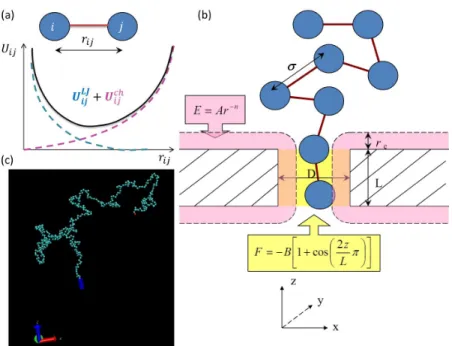
cylindrical void with lengthLand diameter w. The pore length wasL= 2σand pore width wasw= 1.6σ, in which σ was the size of the monomer. These dimensions were maintained throughout the simulations unless specified otherwise.
The polymer chain was represented as a string of beads connected by a spring using a coarse-grained bead-spring model. The membrane consists of fixed and regularly arranged atoms, which were considered a steric hindrance for the monomers. The monomers could not cross the membrane except through the pore. We used a bond potential connecting monomersi and j described by Uij =UijLJ +Uijch, in which the first
term is a trunked-shifted Lennard-Jones potential:
UijLJ =
4ij σ rij 12
− σ rij
6
+1 4
rij≤21/6σ,
0 rij≥21/6σ.
and the second term is a finite extensible nonlinear elastic bond potential:
Uijch=−1 2kR 2 0ln " 1− r ij R0 2# (2.44)
wherek= 30.0/σ2is the spring constant andR
0= 1.5σis the maximum chemical bond length at which
the elastic energy of the bond becomes infinite.
The motion of monomers is described by the Langevin Equation:
mir¨i=−∇Uijmiζr˙i+fi(t)
, whereUij is the interaction potential between the ith and jth monomers at the bound potential(eq.2.44),
and mi,ri and ζi are the mass, coordinate, and friction coefficient, respectively. All monomers were given
the same mass, size, and friction coefficient. Here, fi(t) is the random force of the ith monomer, which is
characterized by correlation functions
hfiα(t)i= 0
hfiα(t)fjβ(t0)i=δijδαβδ(t−t0)2kBT ζ
in whichαandβ denote Cartesian coordinates.
Simulations were performed in the NVT ensemble with kBT = 1.0 using an integral time step ∆t =
0.01τLJ, in whichτLJ =σ m 1/2
, which is the Lennard-Jones time. The simulation systems have periodic boundaries at in the directions other than x(i.e., the translocation direction). We used the reduced units and the friction coefficient wasζ= 4τLJ−1. A pulling force was put on monomers inside the pore only, with a strength ofF = 8.0kBT
σ cos πx
L
, wherex∈
−L 2,
L 2
mentioned in this manuscript were Brownian simulation of 3D ideal chain translocations. The length of chain was 800 monomers. The thermal statistics were done by running the same initial conformation 400 times and for a total of 600 different initial conformations.
Section 2.4: Results and discussion
The section will show the dependence of the ensemble average translocation time, tm , and fluctuations
of δt and ∆t on both the monomer index, m, and the pulling force, F. We compared both an analytical approach and a Lagenvin dynamics simulation to study this question.
In the simulation, an ensemble of fully relaxed polymer chains are anchored at the pore on the cis side with various initial conformations, Γ1,Γ2, . . .For each of those conformations, Γi, we make identical copies
in the simulations, Γi
1,Γi2, . . .. The translocation of each copy undergoes a different thermal history, and we
recorded the translocation time for each monomertm Γij
. The average translocation time was calculated by
tm=
Σi,jtm(Γij)
Σi,j
. Within the simulation, we analyzed the thermal fluctuation,δt, by taking the standard deviation of the distribution of the translocation time, i.e.,
δtm(Γi) =
s
Σj(tm(Γij)−tm(Γi))2
Σj
, wheretm(Γi) =
Σjtm(Γij)
Σj , and then average it over all conformations
δtm=
Σiδtm(Γi)
Σi
. The fluctuation of translocation time due to the variations of initial conformations is calculated by
∆tm=
s
Σj(tm(Γi)−tm)2
Σi
. Details of the simulation protocol are provided in Section.2.3.
results. The identification of conformation is referred to as fingerprinting, i.e., tm is a fingerprint of initial
conformation,
tm=
ζ·b F (
1 b
Z m
0
R(m01)dm1)
.
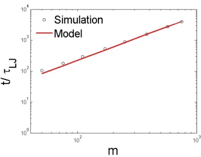
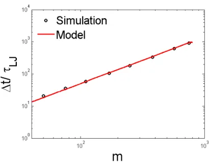
In simulations, initial conformations of polymer chains are randomly distributed, so the average translo-cation time corresponds to an average of all possible initial conformations. In Figure 2.4, we compare how the monomer index depends on this translocation time for the model and simulations. The model predicts the average translocation time using the formula,t(m)≈ ζ·lbond
F m
1+ν (see Section.2.2.2). We conclude that
predictions of average translocation time from the model agree with the simulations.
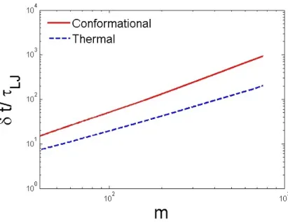
The magnitude of thermal fluctuation of the translocation time can be obtained only through Langevin Dynamics simulation and asymptotic analysis. First, we calculated the standard deviation of the transloca-tion time for polymer chains featuring the same initial conformatransloca-tion within the simulatransloca-tion. Then the devia-tions were averaged over different initial conformadevia-tions. We learned from the simulation that the dependence of the thermal fluctuation on the monomer index can be described asδtm∝mβ, where β(simulation)= 1.16.
In Section.2.2.2, we found the theoretical asymptotic prediction of the thermal fluctuation of the transloca-tion time wasδtm∼m0.5t0.5for the ideal polymer chain. If we assumed the average translocation time from
the asymptotic result wastm∝m1.50, then we obtained β(model)= 1.25, which is larger than the exponent
obtained through simulation. However, if we used the average translocation time of our simulation value tm ∝m1.36 instead of the asymptotic one, then the exponent of the thermal fluctuation becameβ = 1.18,
which is quite close to the simulation value ofβ.
The other component of fluctuation, conformational fluctuation, ∆tm, is calculated in the simulation
as the standard deviation of the thermally averaged translocation times for various initial conformations. We also calculated the translocation time as the numerical solution of translocation time under our model for each initial conformation in the absence of thermal perturbations. The scaling factor fitting from the simulation ∆tm∝mγ,γ(simulation)= 1.5, matched our numerical calculation based on our modelγ(model)=32
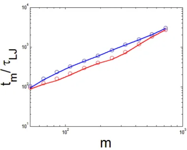
for the ideal polymer chain (Section.2.2.2). Our results also show that the conformational fluctuation of the translocation time surpasses the thermal fluctuation as the conformational fluctuation increases faster with m (Figure 2.5).
chains. Third, our model assumed that the moving section (includingm0−mmonomers) adopted a straight conformation. This assumption requires higher order corrections.
Section 2.5: Concluding remarks
We introduced a theoretical model to calculate the translocation time of each monomer for a given initial conformation of the polymer chain. We compared the theoretical predictions and simulation results for individual initial conformations and demonstrated that translocation time is sensitive to initial conformation of the chain, and thus can be used to fingerprint the chain conformation prior to translocation. The difference in the predicted translocation times between the model and the simulation for a single conformation was small compared to the difference between various initial conformations. Therefore, our theory can be used to characterize individual chain conformations.
The scaling dependence of the average translocation time of the mth monomer was derived using the long chain limit and characterized by the asymptotic value of the exponent 1 +υ= 1.5. Comparison of the model prediction to the simulation shows that analytical results of thermal/conformational broadening are in reasonable agreement. In addition, our model predicted the scaling law for thermal and conformational fluctuation and the correlation between initial conformation and translocation time. These predictions were also well supported by simulations.
In this work, we also investigated the ensemble average translocation time’s dependence on the monomer index using both numerical calculationtm ∝m1.42 and simulation tm∝m1.36, and compared these values
with the asymptotic prediction of tm ∝m1.5 for the ideal polymer chain with a scaling exponent of ν =
0.5. Using our model, we also studied the scaling properties of thermal fluctuation, δtm ∝ m0.5t0.5, and
conformational broadening, ∆tm∝m1.5, which matched the simulation results within uncertainty.
Section 2.6: Figures
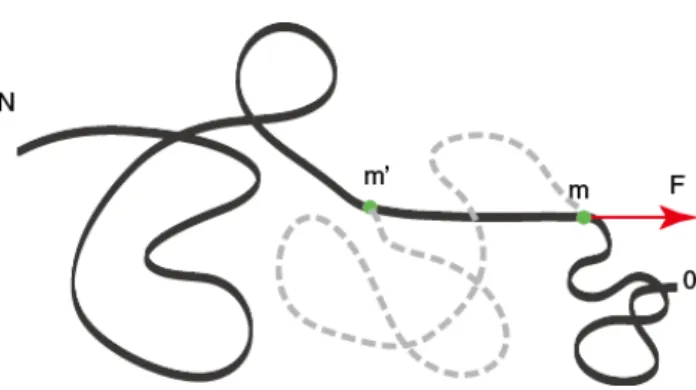
Figure 2.1: Forced translocation of the polymer through the nanopore resembles pulling a rope at a fixed location. Heremis the index of the translocating monomer (inside the pore), andm0is the furthest monomer affected by the applied force. Only the aligned strand is subject to the pulling force (i.e., the section between themth and m0th monomer). The dotted curve is the original conformation of the polymer chain prior to
Figure 2.2: The setup of 3D Langevin Dyanmics simulation of translocation. (a) The bond potential con-necting beads iandj isUij=UijLJ+Uijch, where the first term is a trunked-shifted Lenard-Jones potential
CHAPTER 3: Single ds-DNA molecules in nanochannels
Section 3.1: Introduction
Like nanopores[12, 19, 110, 91, 57], nanochannels also can be utilized for the determination of genome information on a per molecule basis.[98, 59, 57, 51, 97] However, the detection technology in those two platforms can be different. In the nanopore system, a digest of electric signals can reveal either the nucleotide sequence on a scale of base pair by the depth of the blockage current or the length of a DNA molecule by the dwell times of the current blockades.[12, 57, 79] The nanochannel platform employs the optical technology to map the genomic information of single DNA molecules, instead of the electric measurements in nanopore practice[97]. The difference is due to the high electrical resistance that a long nanochannel possesses (as nanochannels are generally longer than nanopores), which makes the axial ionic conductance of the nanochannel less sensitive to the presence of DNA molecules.
When a single DNA molecule is confined to a nanochannel, it can be stretched to about half of its full length.[97] Such a linearization of the DNA provides a map from the positions of the base pairs to the genomic order of them. The enzyme cuts the DNA molecule into fragments on the sites of specific motif. The fluorescent-stained fragments relax and diffuse apart and their lengths are measured through the optical imaging. Despite of the restriction enzyme cutting[98] in nanochannels, nick-labeling[122] DNA and denaturation mapping[95] of DNA also use the optical technology for determine the relative location of the target motifs. Similar to Sangers method[104], the optical mapping within a nanochannel provides the length measurement of the fragmented DNA molecules and therefore offers the frame for assembling the genome. However, the optical mapping has the advantage of preserving the ordering of the fragments, as the fragments within the nanochannel cannot interpenetrate each other due to the excluded-volume interaction. The assembly of genome from the digest of the lengths of the DNA fragments requires a thorough understanding of the statics of single DNA molecules confined to the nanochannel, such as the dependence of the length on the contour length and the nanochannel width. This problem will be addressed in the first part of this chapter. 1
The entry of DNA from the reservoir into a nanochannel is driven by the high field in the nanochan-nel and in the immediate vicinity of the nanochannanochan-nel entry.[82] The strength of the electric field decays 1This chapter is adapted from the theoretical part of a manuscript, which is contributed by Yanqian Wang, Sergey Panyukov
quadratically with the distance from the nano-entrance increases, only the portion of the electric field imme-diately surrounding the entrance contributes to the nanochannel entry. Experimental and theoretical studies have found that this electric field outside nanochannel has small additional contribution to facilitate the nanochannel entry.[126, 83] Driving a micron-sized DNA molecule such as T4-phage DNA into a nano-scale channel requires a strong electric field to overcome the entropic barrier. The strong electric field results in a fast migration speed that impedes the trapping of the DNA within the nanochannel. There have been a number of experimental efforts [25, 18, 65, 123, 62] to slow down the DNA molecule: Their methods included increasing the solution viscosity, decreasing its temperature, and introducing nanochannel arrays. The un-derstanding of the driving force on the DNA is crucial in developing strategies to slow down the molecule and many efforts were made on the related research.[63, 44, 126, 35, 116] The study of this electric-induced force, i.e. the electro-hydrodynamic force will be also presented in this chapter.
Section 3.2: Physical properties of ds-DNA molecule
We model double-stranded DNA (ds-DNA) stained with an intercalating dye, as a semiflexible chain with persistence lengthlp '50nm, backbone diameter a'2nm and contour lengthL ( 21µm for λ-DNA and
72µmfor T4 DNA).[81, 93, 33] The ds-DNA backbone is negatively charged and is surrounded by positively charged counterions dissolved in a polar aqueous solvent. The bare charge of the chain backbone is two elementary charge e per basepair (bp) with the bare linear charge density 2e/bp(5.9e/nm). The counterion condensation process reduces the net charge of the backbone to the Manning value of e/lB , where lB is
Bjerrum length, which is defined as the distance at which two elementary charges interact with electrostatic energy equal to the thermal energykBT , wherekB is Boltzmann constant andT is absolute temperature
lB =e2/(kBT) (3.1)
The Bjerrum length islB = 7 ˚A in water at room temperature with dielectric constant'80.
Correspond-ingly, the counterion (Onsager-Manning) condensation reduces the bare linear charge density by the factor of 4 from 2e/bp to 0.5e/bp= 0.14eA˚−1.
The remaining uncondensed mobile counterions are localized within double-layer ”coat” around backbone with thickness equal to the Debye length. The Debye screening length depends on the concentration cs of
monovalent ions in the electrolyte solution