ADVANCED ANALYSIS METHODS FOR LARGE-SCALE STRUCTURED DATA
Fan Zhou
A dissertation submitted to the faculty at the University of North Carolina at Chapel Hill in partial fulfillment of the requirements for the degree of Doctor of Philosophy in the
Department of Biostatistics in the Gillings School of Global Public Health.
Chapel Hill 2019
Approved by: Hongtu Zhu Haibo Zhou Lisa Lavange Fei Zou
c 2019 Fan Zhou
ABSTRACT
Fan Zhou: Advanced Analysis Methods For Large-Scale Structured Data
(Under the direction of Hongtu Zhu and Haibo Zhou)
In the era of ’big data’, advanced storage and computing technologies allow people to build and process large-scale datasets, which promote the development of many fields such as speech recognition, natural language processing and computer vision. Traditional approaches can not handle the heterogeneity and complexity of some novel data structures. The target of this dissertation is to develop new statistical models to solve all kinds of real-world problems based on structured data from different areas.
Three different data structures are discussed in this dissertation. In the first part of the dissertation, we introduce a novel data sampling scheme: muti-group association data, which is widely adopted by recent medical studies with multi-class disease outcomes. We develop a general regression framework for the secondary phenotype analysis using multi-group data to correct the estimation bias caused by the uneven sampling rates of different sub-groups.
The second data type being included is the graph-based data, i.e. the network data. In this dissertation, we discuss the graph-based semi-supervised learning problem with nonignorable missingness, which is ignored by most previous studies. We do both simulation and real analysis using citation networks to show the necessity of doing bias correction when there exists nonignorable nonresponses.
ACKNOWLEDGEMENTS
I would like to thank my advisors, Dr. Hongtu Zhu and Dr. Haibo Zhou, for your mentoring through my whole PhD career. Your guidance has helped nurture my independent thinking, academic sense, passion in exploring unknown fields, as well as self-learning and collaboration ability.
I would also like to thank Dr. Lisa Lavange, Dr. Fei Zou and Dr. Yen-Yu Ian Shih for serving as my committee members. Your valuable comments and suggestions really help.
TABLE OF CONTENTS
LIST OF TABLES . . . xi
LIST OF FIGURES . . . xii
CHAPTER 1: INTRODUCTION . . . 1
CHAPTER 2: LITERATURE REVIEW . . . 3
2.1 Structured Data . . . 3
2.1.1 Multi-Group Association Data . . . 3
2.1.2 Graph-Based Data . . . 5
2.1.3 OD flow data . . . 8
2.2 Secondary Phenotype Analysis . . . 10
2.2.1 Inverse Probability Weighting . . . 11
2.2.2 Likelihood-based Methods . . . 12
2.2.3 Semiparametric and Estimating Equation Methods . . . 14
2.3 Non-ignorbale Non-response . . . 16
2.3.1 Selection models . . . 20
2.3.2 Pattern-mixture models . . . 22
2.3.3 Pseudo-likelihood method . . . 23
2.4 Spatial-Temporal Predictions . . . 24
CHAPTER 3: ANALYSIS OF SECONDARY PHENOTYPES IN MULTI-GROUP ASSOCIATION STUDIES . . . 29
3.1 Introduction . . . 29
3.2.1 Data Structure and Notation . . . 32
3.2.2 Model Setup . . . 32
3.2.3 Estimation . . . 34
3.2.4 Extension to Binary Secondary Outcome . . . 37
3.2.5 Extension to Multi-phase Scenario . . . 38
3.3 Simulation Studies . . . 39
3.3.1 Two-SNP Setup . . . 40
3.3.2 Multiple-SNP Setup . . . 43
3.4 The Alzheimer’s Disease Neuroimaging Initiative Data . . . 44
3.4.1 GWAS analysis . . . 44
3.4.2 Results . . . 45
3.5 Discussion . . . 48
CHAPTER 4: GRAPH-BASED SEMI-SUPERVISED LEARNING WITH NONIGNORABLE NONRESPONSES . . . 51
4.1 Introduction . . . 51
4.2 Model Description . . . 52
4.3 Estimation . . . 54
4.3.1 Identifiability . . . 55
4.3.2 Estimation Approach . . . 57
4.3.3 Algorithm . . . 60
4.4 Experiments . . . 61
4.4.1 Simulations . . . 63
4.4.2 Real Data Analysis . . . 64
CHAPTER 5: STOD: SPATIAL-TEMPORAL ORIGIN -DESTINATION PREDICTION MODEL . . . 67
5.1 Introduction . . . 67
5.3 STOD Framework . . . 71
5.3.1 Spatial Adjacent Convolution Network . . . 72
5.3.2 Temporal Gated CNNs . . . 75
5.3.3 ST-Conv blocks . . . 77
5.3.4 Periodically Shifted Attention Mechanism . . . 79
5.3.5 Final prediction layer . . . 81
5.3.6 Optimization . . . 82
5.4 Experiment . . . 82
5.4.1 Dataset Description . . . 82
5.4.2 Evaluation Metric . . . 83
5.4.3 Compared Methods . . . 83
5.4.4 Experiment Setting . . . 84
5.4.5 Results . . . 85
5.5 Discussion . . . 87
APPENDIX A: APPENDIX FOR CHAPTER 2 . . . 89
A.1 Proofs and Explicit forms . . . 89
A.1.1 Proof of (3.2) . . . 89
A.1.2 Proof of (3.3) . . . 89
A.1.3 Proof of (3.14) . . . 90
A.2 D with more than three categories . . . 91
A.3 Simulations with multiple SNPs . . . 92
A.3.1 Setting One . . . 92
A.3.2 Setting Two . . . 93
A.4 The Alzheimer’s Disease Neuroimaging Initiative Data . . . 94
A.4.1 Sample . . . 94
A.4.2 MRI Acquisition and Image Preprocessing . . . 94
A.5 The Boxplots of the log volumes of the left and right hippocampi in ADNI1
and ADNI2, ADNI GO . . . 95
APPENDIX B: APPENDIX FOR CHAPTER 3 . . . 97
B.1 Theorem Proofs . . . 97
B.1.1 Lemma and proof . . . 97
B.1.2 Proof of Theorem 4.1 . . . 98
B.1.3 Proof of Theorem 4.2 . . . 100
LIST OF TABLES
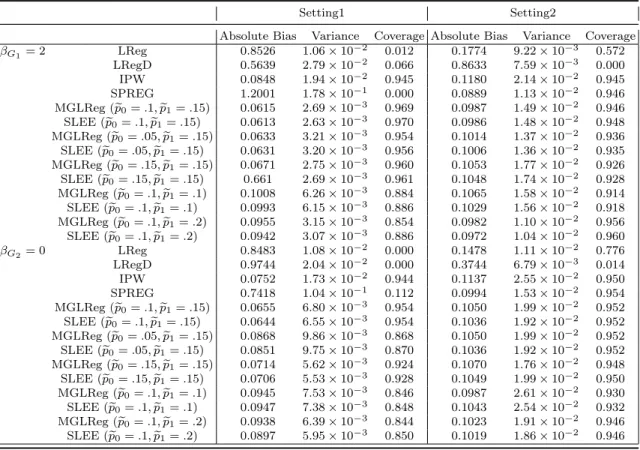
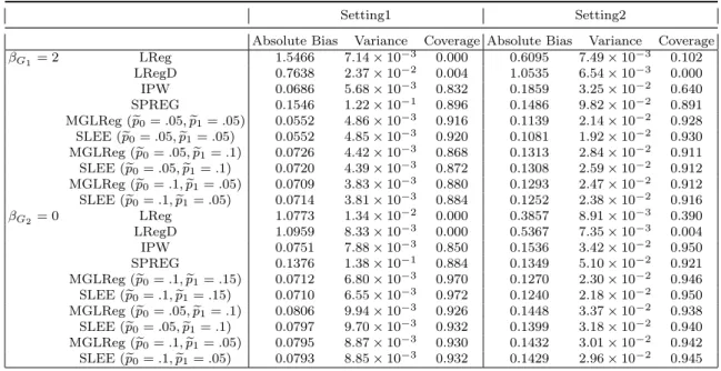
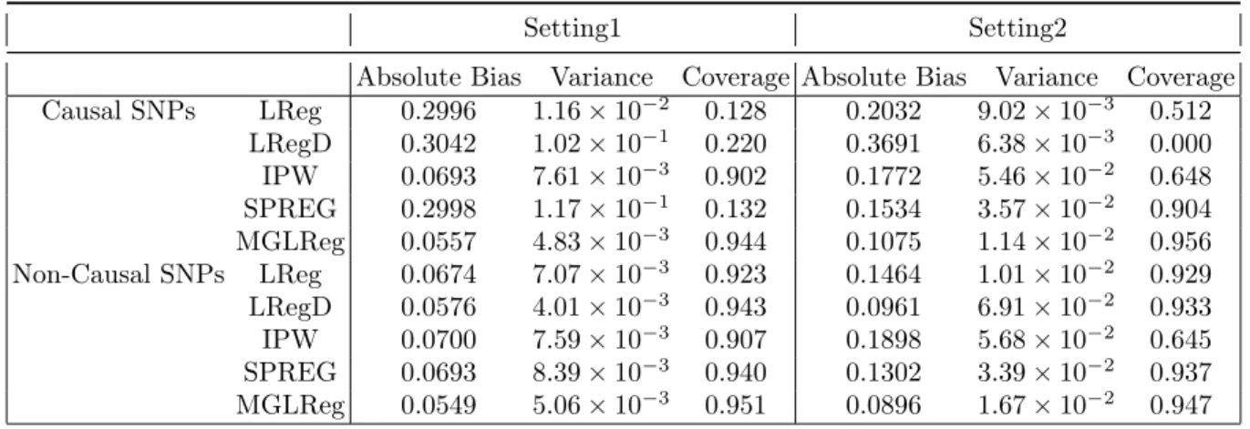
3.1 Estimation biases, variances, and 95%coverage rates of βbG for pA= 0.3 . . . 42 3.2 Estimation biases, variances, and 95% coverage rates of βbG for rare disease case 43 3.3 Mean estimation biases, variances, and 95% coverage rates of Causal and
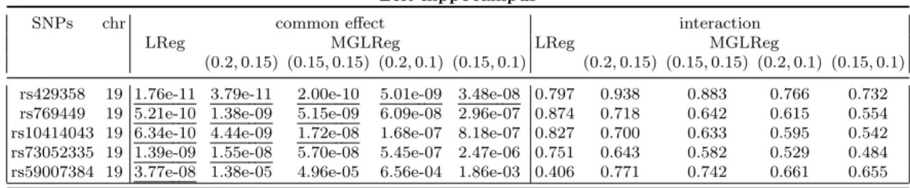
Non-causal SNPs . . . 44 3.4 Top SNPs andp−values for association tests with the left and right
hippocam-pus volumes . . . 46
LIST OF FIGURES
3.1 The heatmaps of−log10(p)-value for three selected SNPs by MGLReg with
different global AD and MCI prevalence rates in the whole population . . . . 47
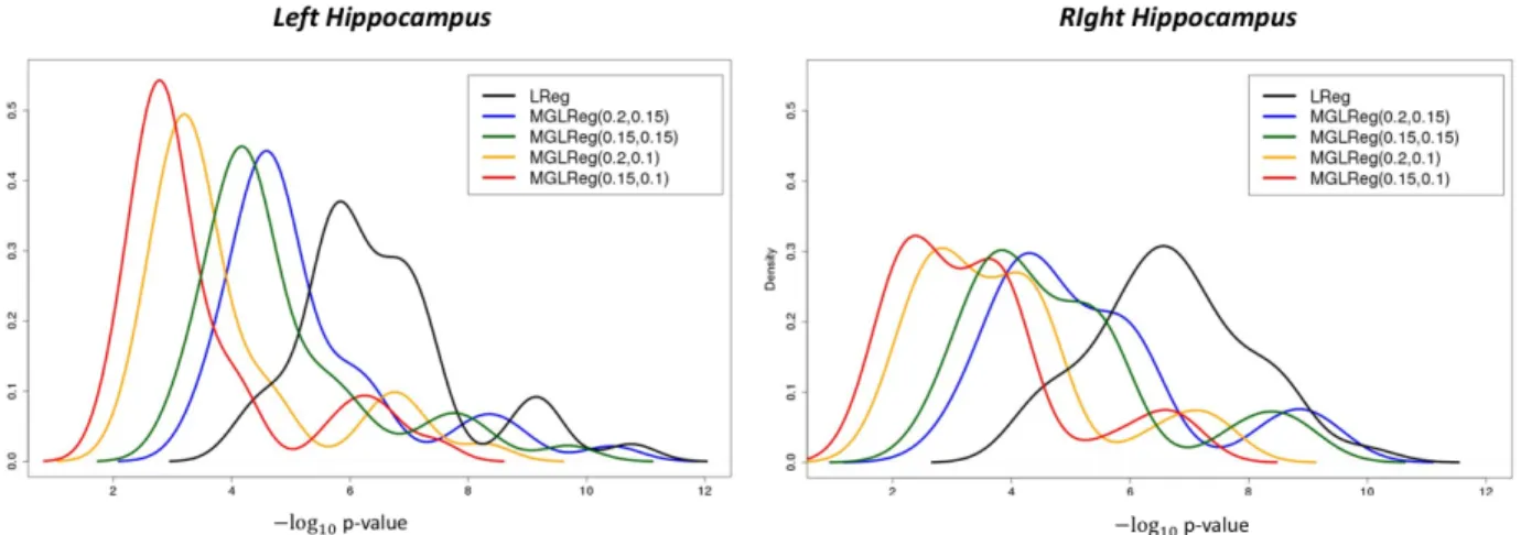
3.2 The density curves of−log10(p)-values of top 50 APOE-region SNPs by each method for the left and right hippocampus volumes . . . 48
3.3 The Manhattan plots of the−log(p)−values by LReg and MGLReg on all 22 chromosomes for the left and right hippocampus volumes . . . 49
3.4 The Manhattan plots of the−log(p)−values by LReg and MGLReg on all 22 chromosomes for the left and right hippocampus volumes . . . 49
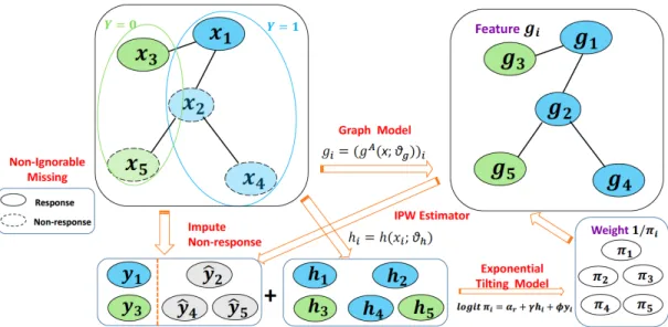
4.1 General Picture of the Joint Estimation Approach . . . 59
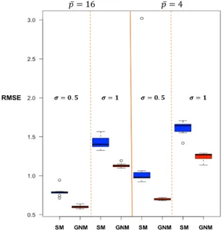
4.2 Boxplot of RMSEs in real data analysis . . . 64
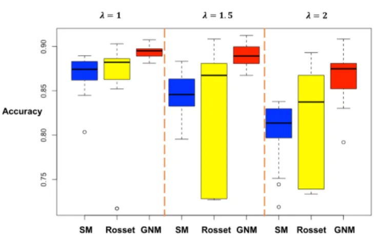
4.3 Boxplot Prediction Accuracy for the simple setup . . . 65
4.4 Boxplot of Prediction Accuracy for the complicated setup . . . 66
5.1 A real example of customer demands from ride-sharing platforms to explain OD flow data from the perspective of dynamic graph adjacency matrices . . 69
5.2 The Architecture of STOD model . . . 71
5.3 An empirical example of passenger requests to illustrate how standard CNN fails to capture the network structure of OD flow data . . . 73
5.4 Working mechanism of spatial adjacent convolution network (SACN) for a target OD flow fromvi tovj . . . 74
5.5 Illustration of temporal gated CNN with kernel size being1×1×2in capturing temporal dependency and reducing sequence length . . . 77
5.6 The architecture of Periodically Shifted Attention . . . 80
5.7 (a) RMSE on testing data with respect to ACN and standard CNN using different kernel sizes. (b) RMSE on testing data with respect to STOD with different p1 and p2 combinations. . . 87
CHAPTER 1: INTRODUCTION
By three different research topics, we explore how to combine useful tools, including both traditional approaches and deep learning architectures, to develop new methodologies in analyzing certain kinds of structured data. The first two topics try to correct the estimation bias that results from unusual sampling designs. The latter two deal with some real-world problems people are interested in generated by network data.
Multi-group design, such as the Alzheimer’s Disease Neuroimaging Initiative (ADNI), has been undertaken by recruiting subjects based on their multi-class primary disease status, while some extensive secondary outcomes are also collected. Analysis by standard approaches is usually distorted because of the unequal sampling rates of different classes. In the first part of the dissertation, we develop a general regression framework for the analysis of secondary phenotypes collected in multi-group association studies. Our regression framework is built on a conditional model for the secondary outcome given the multi-group status and covariates and its relationship with the population regression of interest of the secondary outcome given the covariates. Then, we develop generalized estimation equations to estimate the parameters of interest. We use simulations and a large-scale imaging genetic data analysis of the ADNI data to evaluate the effect of the multi-group sampling scheme on standard genomewide association analyses based on linear regression methods, while comparing it with our statistical methods that appropriately adjust for the multi-group sampling scheme.
approach. We further use graph neural networks (GNN) to model nonlinear link functions and then use a gradient descent (GD) algorithm to estimate all the parameters of GNM. We propose a novel identifiability for the GNM model with neural network structures, and validate its predictive performance in both simulations and real data analysis through comparing with models ignoring or misspecifying the missingness mechanism. Our method can achieve up to 7.5% improvement than the baseline model for the document classification task on the Cora dataset.
CHAPTER 2: LITERATURE REVIEW
In this chapter, we review some existing representative works related to the topics covered in this dissertation. In section 1.1, we introduce three unusual data types: muti-group association data, graph-based data and origin-destination flow data. We briefly discuss the research problems people are interested in and the accompanying statistical challenges when analyzing these three kinds of structured data. In section 1.2, we review a large set of literature on the development of statistical methods to eliminate the selection bias related to ascertainment in case-control studies for secondary trait analysis. In section 1.3, we review the main approaches to obtain unbiased parameter estimations in the presence of nonignorable missingness. In section 1.4, we go through the developing history of prediction models applied to dynamic spatial-temporal data.
2.1 Structured Data
2.1.1 Multi-Group Association Data
Case-control (Cornfield, 1951) is a special design of observational study, which recruits two groups of people with potentially different outcomes to certain diseases to explore their association with some exposure variables of interest. The case-control study follows a retrospective design since the primary outcome of each individual is known before it being enrolled and all the covariate information can be retrieved.
follow different sampling schemes, where the first stage is equivalent to a standard case-control sample and subjects in the second stage are subdivided into four groups: two case groups (diseased and exposed/unexposed) and two control groups (normal and exposed/unexposed). The two-stage design is more efficient and flexible because the sample sizes of the four subgroups can vary with the disease and exposure rates. Breslow and Cain (1988) propose an irregular logistic regression for the two-stage case-control design, the efficiency of which is maximized when the exposure rate is rare. Flanders and Greenland (1991) introduces a pseudo-likelihood approach to analyze the data acquired from two-stage case-control studies.
Although case-control design has been widely used in biological studies, they are insufficient for many complex diseases, such as Alzheimer’s disease and breast cancer. These diseases may have multiple subtypes with distinct morphologies and clinical implications. To recruit enough people for each disease subtype, multi-group design can be employed to sample subjects within different groups in different proportions from the whole population. One typical example following the multi-group design is the Alzheimer’s Disease Neuroimaging Initiative (ADNI), which has three main groups: Alzheimer’s disease (AD), mild cognitive impairment (MCI), and elderly controls (NC). The major goal of ADNI data set is to promote the development of longitudinal, multi-site, imaging-genetic methods in analyzing Alzheimer’s disease. Patients from the three groups are non-randomly sampled with different probabilities where a total of 800 subjects including 200 normal controls, 400 individuals with MCI, and 200 subjects with mild AD are recruited by ADNI1. More than 50% subjects in the sample are with MCI since researchers want to explore more about the transition mechanism from MCI to AD while no more than 15% of people older than 55 are in MCI status in the whole population. ADNI has gone though four phases from ADNI1, GO, 2 to ADNI3 from 2004 until 2016 and the whole sample size is extended to over 1700. A new cohort Significant Memory Concern (SMC) is added since ADNI2.
surgery for thyroid cancer at Mackay Memorial Hospital between January 2001 and May 2012 are recruited to build the sample. The TMA data is usually generated by the tissue sections cut from both normal and tumor samples. The proportion of subjects in the sample with more severe cancer stages are much higher than those in the whole population, which makes the TMA dataset a non-random sample.
Similar to the case-control design, estimations by standard models using the muti-group association data can be extremely misleading. In this dissertation, we build a general framework to properly correct the sampling bias when analyzing secondary phenotypes in multi-group association studies.
2.1.2 Graph-Based Data
Graphs can be used to represent either symmetric or asymmetric relations between a group of discrete objects. With technology development and population growth, large-scale graph-based datasets are generated to solve all kinds of real-world problems.
Graph-based semi-supervised learning problem has been increasingly studied, the goal of which is to predict the node responses of all the unlabelled vertexes (such as documents) in a graph (such as a citation network) based on only a small subset of observed ones. The labelling information is usually smoothed over the graph via some form of explicit graph-based regularization.
A popular method is to use the graph Laplacian regularization to learn node represen-tations, such as label propagation (Zhu et al., 2003), manifold regularization (Belkin et al., 2006) and deep semi-supervised embedding (Weston et al., 2012).
where the generation of random walks and the main semi-supervised classifier are built and optimized individually. Yang et al. (2016) proposes a novel graph-based semi-supervised learning framework. Different from the above two-step procedures, the network embedding and the final classification model are jointly trained by an end-to-end architecture. The graph embedding and hidden representation learned from the classifier are concatenated to feed into the final prediction layer.
In the past few years, more efforts have been devoted to developing deep learning models to capture the spatial information of network data (Bruna et al., 2013; Henaff et al., 2015; Duvenaud et al., 2015; Li et al., 2015). They either pay attention to problem-specific specialized architectures or utilize graph convolutions known as spectral graph theory. Defferrard et al. (2016) designs a localized convolution network for general graph structures. The lower layers of the network is convolutional in the sense that the same local filter is applied to each graph vertex and its neighboring nodes. Then a global pooling procedure combines the features captured by a multi-layer propagation from all the vertexes.
We consider a weighted graph structure consisting of an undirected (or directed) graph
G = (V, E) as well as an adjacency matrix A = (aij), where aijs’ are nonegative edge
weights, V = {v1, . . . , vN} is a set of |V|= N vertices, and E is a set of edges. Moreover,
(vi, vj) ∈ E ⊂ V ×V is an edge equipped with an nonegative weight aij. The adjacency
matrix A= (aij)∈RN×N encodes the node connections. x∈RN×c is the node-level signals
where cis the length of feature vectors.
aAn widely-used operator in spectral graph analysis is the graph Laplacian (Chung and Graham, 1997). Formally, the graph Laplacian given the adjacency matrix A is defined as L = IN −D−
1 2AD−
1
2 where D ∈ RN×N is a diagonal degree matrix with Dii = P
jaij. L=UTΛU is the eigenvalue decomposition of Lwith U being the matrix of eigenvectors and
Λ =diag([λ0, λ1, . . . , λN−1]) being the diagnal matrix containing eigenvalues. We consider
spectral convolutions on graphs defined as the multiplication of the input matrix x∈RN×c
function of the eigenvalues of L, i.e. gθ(Λ). Hammond et al. (2011) suggests that gθ(Λ) can
be well-approximated by a truncated expansion in terms of Chebyshev polynomials Tk(x) up
toK-th order:
gθ(Λ) = K−1
X
k=0
θkTk(Λ) (2.1)
The Chebyshev polynomials are recursively defined as Tk(z) = 2zTk−1(z)−Tk−2(z) with T0 = 1 and T1 =z.
The spectral graph convolutions at the l-th layer incorporated with input mlt ∈ RN×cl can be modified as:
gθ∗mlt≈ K−1
X
k=0
Tk( ˜L)mltWl (2.2)
where L˜ = 2
λmaxL−IN with λmax being the maximum eigenvalue of the Laplacian matrix.
Wl∈Rcl×d is the GCN projection matrix to learn. Assuming x˜k= Tk( ˜L)x, by the recurrence
relations we have x˜k= 2 ˜Lx˜k−1−x˜k−2 with x˜0 =x and x˜1 = ˜Lx.
Kipf and Welling (2016) simplify the graph convolution networks proposed by Defferrard et al. (2016) to highly increase the training efficiency and obtain a higher prediction accuracy. The layer-wise transformation is defined as:
f(H(l), A) = σ(AH(l)W(l)) (2.3)
where W(l) is a weight matrix for the l-th layer and σ(·) is a non-linear activation function such as the ReLU. H(0) = X serves as the input and H(L) =Z is the final output when there are in total Llayers. Despite the simple structure the proposed operation, the model is powerful in capturing the graph-based spatial information.
There are two main limitations of the operation above. One is the multiplication of A
Another limitation is that A is not normalized and multiplication with A will keep changing the scale of the output representations at each layer. Therefore, Kipf and Welling (2016) normalize A to make the row sums to be one, i.e. D−1A, where D is the diagonal
matrix summing up each row of A. Multiplying with D−1A is equivalent to take a weighted
sum over the neighboring grids and the center grid itself. A more advanced way is to use a symmettic normalization D−1/2AD−1/2 (as this no longer amounts to mere averaging of neighboring nodes). With the normalization of the the mutliplication, (2.3) is modified to
f(H(l), A) =σ( ˆD−12AˆDˆ− 1
2H(l)W(l)) (2.4)
where Aˆ=A+I, where I is the identity matrix and Dˆ is the diagonal node degree matrix of ˆ
A. The propagation rule could be seen as the first-order approximation of localized spectral filters on graphs (Defferrard et al., 2016).
2.1.3 OD flow data
dynamic OD flow maps as a sequence of graph snapshots G = {G1, . . . , GT}. With the
OD flow network at each time t∈ {1, . . . , T}, we can define a weighted graph Gt= (V, Ot)
with a fixed vertex set V ={v1, . . . , vN}representing |V|=N urban regions. The dynamic
adjacency matrixOt= (oijt )∈RN×N describes flow amounts within all N2 OD flows, where oijt represents the flow amount from node vi to node vj at timestamp t.
Many efforts have been devoted to developing traffic flow prediction models in the past few decades. Before the rise of deep learning, traditional statistical and machine learning approaches dominate this field. These methods are usually built on linear transformations, so they often ignore non-linear correlations among the OD flows. Some other methods further use additional external features obtained from feature engineering, but they fail to automatically extract the spatial representation of OD data. Moreover, they roughly combine the spatial and temporal features when fitting the prediction model instead of dynamically model their interactions.
The development of deep learning technologies brings a significant improvement of OD flow prediction by extracting non-linear latent structures that cannot be easily discovered by feature engineering. For instance, convolutional operations are often used to capture more complicated spatial patterns in the OD flow data, most of which treat each Ot as an
image. In this case, some nearby OD flows inOt covered by a single CNN kernel may not be
2.2 Secondary Phenotype Analysis
In this section, we review the existing methods for secondary phenotype analysis. We will focus on the case-control design since almost all the existing methods are designed for the two-group situation, where both the binary disease status and some secondary phenotypes are collected.
In case-control studies, subjects of disease and control groups are selected with different probabilities from the whole population. Therefore, fitting a standard regression model is statistically biased when analyzing the secondary phenotypes. There are several ways to correct the estimation bias caused by the uneven sampling rates of the two groups. Before moving to the details of these approaches, we introduce some important notations first. Let
D be the primary binary outcome (case-control status) and Y be the secondary outcome (which could be either continuous or categorical). X denotes the set of covariates to analyze. The simplest method is to fit a standard regression model using a subset of observations. All these naive approaches can fall into four broad categories depending on the groups of subjects being included:
1. Regress Y overX using control subjects only.
2. Regress Y overX using case subjects only.
3. Regress Y overX using the entire sample.
4. Include the case-control status D as an additional covariate in the regression models.
and only ifY ⊥D|X. (4) may yield flawed conclusions, since the associations between the secondary outcome and an exposure of interest in the case and control groups can be quite different from that in the underlying target population (Tchetgen Tchetgen, 2014).
Faced with the increasing demand in analyzing secondary traits on case-control sample, a number of well-designed modified statistical approaches are proposed. All these methods can be roughly divided into three main classes: (1) Inverse Probability Weighting (IPW) methods. (2) Likelihood-based methods. (3) Semiparametric efficient estimating methods. 2.2.1 Inverse Probability Weighting
Various weighted likelihood approaches, such as the inverse probability weighting (IPW), have been widely used (Richardson et al., 2007; Monsees et al., 2009; Schifano et al., 2013; Sofer et al., 2017) to correct sampling bias. The IPW-based approaches replace the normal log-likelihood function by a weighted sum using weights wi given by the reciprocal of the
selection probability for each subject in the case-control sample. We let the target of inference be fβ(Y|X) with β including all the parameters related to the the conditional mean model.
If the total sample size is N, the weighted log-likelihood function is defined as:
l(β) =
N
X
i=1
1
wi
logfβ(Yi|Xi) (2.5)
which is proved to provide unbiased estimation of β and appropriate type-one error rates. Schifano et al. (2013) extends the IPW approach to multiple-response situation, improving the statistical power by borrowing strength across outcomes with a one degree of freedom test and jointly estimating the outcome-specific exposure effects when the secondary phenotypes are positively correlated. Suppose yi = (yi1, . . . , yiM) denotes the M-dimension correlated continuous phenotypes andσ2
i being the phenotype-specific variance, the weighted estimating
equations is defined as:
N
X
i=1
wiXTi R
−1
(yi
σi
and
N
X
i=1 wi{
yij σj(
yij σj −x
T
i β)−1}= 0, j = 1, . . . , M (2.7)
where R is the working correlation matrix and
Xi =
xT
i 0T . . . 0T
0T xT
i . . . 0T
..
. . .. ... 0T 0T . . . xTi
The weight wi equals to the global prevalence divided by the sample-level group proportions.
Schifano et al. (2013) proves that the proposed estimating equation is unbiased.
Sofer et al. (2017) points out that IPW is inefficient because of ignoring the data generating mechanism. To address this issue, they propose a novel class of estimators which combine traditional IPW with specification of the disease outcome probability model via a mean zero control function. The control-function assisted IPW estimating equations is defined as follows:
U(β) =
N
X
i=1
1
π(Di)
(h1(Xi)[Yi−g−1{µ(Xi;β)}]−h2(Xi, Di)) = 0 (2.8)
where π(Di) = P r(Si = 1|Xi, D) and [Y|X] = g−1{µ(X;β)} are the population-level
conditional mean model. Si is a binary variable indicating whether a subject is selected into
the sample. h1(X, D), h2(X, D) are the control functions which depend on the disease model
and satisfies {h2(X, D)/π(D)|X, S = 1} = 0. In this case, the inverse probability weight
becomes h2(X, D)/π(D) with mean zero sum.
In practice, IPW-based methods are usually inefficient since some information related toD
is not fully utilized. Likelihood-based and semiparametric estimation approaches could solve this problem to some extent, the details of which are discussed in the following subsections. 2.2.2 Likelihood-based Methods
conditional distribution of D andY given X when the sampling rates for the two groups are known. Jiang et al. (2006) carries out an extensive investigation of efficiency and proves that the semi-parametric maximum likelihood methods are theoretically more efficient than the weighted likelihood methods.
Lin and Zeng (2009) introduces a retrospective likelihood function by explicitly condition-ing on the samplcondition-ing scheme. If Y is a continuous outcome, a linear regression model could be used when assuming Y givenX follows a normal distribution with mean β0 +β1X and varianceσ2. When Y is the binary outcome, we model Y|X by a logistic regression:
P(Y = 1|X) = e
β0+β1X
1 +eβ0+β1X (2.9)
Moreover, another logistic regression is used to describe the relationship between D and (Y, X)as:
P(D= 1|X, Y) = e
γ0+γ1X+γ2Y
1 +eγ0+γ1X+γ2Y (2.10)
Because the sampling is conditional on the case-control status, the likelihood function takes the retrospective form:
N
Y
i=1
P(Di = 1|Xi, Yi)P(Yi|Xi)P(Xi) P(Di = 1)
Di
P(Di = 0|Xi, Yi)P(Yi|Xi)P(Xi) P(Di = 0)
1−Di
(2.11)
where P(Di = 1) =PyPxP(Di = 1|x, y)P(y|x)P(x),P(Di = 1) = 1−P(Di = 0). Lin and
Zeng (2009) proposes a profile-likelihood approach to eliminate the nuisance parameters from the potential high-dimensional probability distribution of continuous environmental covariates. Specifically, they treat the distribution of x as discrete point masses pi = p(xi) based on
the N finite observations in the case-control sample. PN
i=1pi = 1 is the added additional
He et al. (2012) uses a gaussian copula approach, allowing more flexible distributions of the secondary outcomeY compared to Lin and Zeng (2009), which works for the multiple-outcome case.
2.2.3 Semiparametric and Estimating Equation Methods
Wei et al. (2013) proposes a robust estimation method for secondary analysis of case-control data by assuming that the secondary trait Y given X follows a homoscedastic regression model, which is defined as
Y =α+µ(X, β) + (2.12)
where α is the intercept andµ is a known function. is the zero-mean error term which is independent ofX.
The method by Wei et al. (2013) allows the model for Y given X to be incorrect, and makes the estimation approach robust. One main assumption of this method is that the disease rate is given or could be well estimated. They pursue a sequential approach to estimate the parameters related to the target regression model Y|X. The details of the algorithm are described in three steps as follows:
1. Estimate the logistic regression of D given (X, Y)and obtain the related parameters κ,
θ1. The logistic model is defined as:
P(D= 1|X, Y) = e
θ0+m(Y,X;θ1)
1 +eθ0+m(Y,X;θ1) (2.13)
On the other hand, κ = θ0 + log(n1/n0)−log(π1/π0) where n1, n0 are the number
of subjects in case and control group, and π1, π0 are global prevalences for the two
groups in the whole population. Prentice and Pyke (1979); Chatterjee and Carroll (2005) demonstrate thatθ1 andκcan be consistently estimated by the standard logistic
regression using the case-control sample. Moreover, it is assumed that a consistent estimation of θ0 could also be obtained by solving an estimating equation.
population. The simplest way to acquire the score function is to take the derivative of the ordinary least squares {Y −α−µ(X, β)}2, making the score funtion to be
L{R(β), X, α, β}=µβ(X, β){R(β)−α} (2.14)
where R(β) =Y −µ(X, β). The score (2.14) is then adjusted to have zero-mean under case-control design.
3. DenoteΩ = (κ, θ0, θ1)and replaceαin the score function byα(β,Ω). Solve the adjusted
score equation and get the estimation of β and hence α.
Song et al. (2016) introduces a set of counter-factual estimation functions under an alternative disease status, and combines the observed and counter-factual estimation functions into a set of weighted estimation equations (WEE). Simulations results demonstrates that WEE is more robust against biased sampling and less sensitive to model misspecification.
Assuming S(X, Y, β)is an estimating function with EY(X, Y, β∗)|X)at true value β∗, the
unbiased counterfactual estimating equation by conditional expectation is defined as:
Sn(β) = N
X
i=1
[S(xi, yi, β)p(di|xi) +Ey˜i[S(xi,y˜i, β)|xi]p(1−di|xi)] = 0 (2.15)
where yi is the observation in the sample and yi˜ is the counter-factual secondary outcome under the alternative disease status. Estimating equation (2.15) remains unbiased when
S(xi,y˜i, β) is non-linear. Another estimation approach is to fit the modelY|X for cases and
controls separately, and then generate pseudo counter-factual observations using the resulting stratified models.
of Y given X in the whole population is defined as:
Y =m(X, β) + (2.16)
where m(·)is a known function and is the zero-mean error term. To relax the assumptions of error distribution and disease rates, the concept of a superpopulation (Ma et al., 2010) is adopted. Under the superpopulation framework, the regression model can be rewritten as:
fYtrue|X(X, y) =η2{y−m(X, β), X} (2.17)
whereη2is an unknown probability density function that has mean0givenX. The case-control
sample could be considered as a random sample from an imaginary infinite superpopulation, where the ratio between disease and normal is N1/N0. N1 and N0 here are group sizes in the
case and control groups, respectively. The joint density of D, Y, X in the superpopulation is defined as:
fX,Y,D(x, y, d) = Nd
N
η1(x)η2(, x)H(d, x, y, α)
ptrue
D (d, α, β, η1, η2)
(2.18)
whereθ = (αT, βT)T is the parameter of interest;η1(·)andη2(·,·)are the nuisance parameters. An efficient estimator can be obtained by solving the semiparametric score equation
N
X
i=1
[S(Xi, Yi, Di)−g{Yi−m(Xi, β)Xi} −(1−Di)v0−Div1] = 0 (2.19)
where S() is the score function and g() is an arbitrary function. It is mentioned in the paper that the proposed estimator is not only efficient for the constructed superpopulation but also the real whole population.
2.3 Non-ignorbale Non-response
a response is labelled depends on not only the observed but also the missing observations (Little and Rubin, 2019). In this case, the non-response cannot be ignored.
With the presence of non-ignorable non-response, disregarding such a missing mechanism may destroy the representativeness of the remaining samples and subsequently lead to significant estimation bias (Baker and Laird, 1988; Diggle and Kenward, 1994; Ibrahim et al., 1999; Molenberghs and Kenward, 2007). We assume that the problem of interest is to unbiasedly learn an outcome model Y|x. Without loss of generality, when y is continuous, we consider a linear model given by
Y =α+xβ+, (2.20)
where = (1,· · · , N)T ∼ N(0, σ2I) and ⊥ x is the error term with zero unconditional mean, that is, E(i) = 0. We let ri ∈ {0,1} be the “labeling indicator”, whereyi is observed
if and only if ri = 1. With the non-ignorable missingness, dropping out missing data can
lead to strongly biased estimates when r depends on y. The parameter estimates will not be consistent since E{i|ri = 1} and E{ixi|ri = 1} are not zero. The missing values could not
be imputed even if we would have consistent estimates since
E{yi|ri = 0, xi;α, β}=
E{yi(1−ri)|xi;α, β}
1−P(ri = 1|xi;α, β)
=α+βTxi−
cov(yi, πi|xi;α, β)
1−E(πi|xi;α, β)
6=α+βTxi.
(2.21) Modeling non-ignorable missingness is challenging because the MNAR mechanism is usual-lyunknown and may require additional model identifiability assumptions (Chen, 2001; Qin et al., 2002; Tang et al., 2003; Ibrahim et al., 2005). Little and Rubin (2019) classifies the approaches dealing with missing data into four different categories:
inaccuracy because the complete cases are not randomly sampled from the whole population (Little and Rubin, 2019).
• Weighting procedures. These methods assign the inverse of estimated response probabilities as weights to the responding units (Robins et al., 1995; Carpenter et al., 2006) when building the likelihood function, but most of these procedures are designed for the missing at random (MAR) mechanism instead of NMAR. Very few methods, such as the one proposed by Deville (2000) and Chang and Kott (2008) can work for the non-ignorable non-response situation. The weighting approaches are usually based on the auxiliary information available for all the subjects, and the conditional probability to respond is always considered as propensity score (Rosenbaum and Rubin, 1983). • Imputation Procedure Another class of methods is to impute missing data by using
observed data (Rubin, 1976; Schafer and Schenker, 2000; Little and Rubin, 2019). These methods are based on the derived fully likelihood function including all the subjects, with non-respondents valued by estimations using information of respondents. The imputation procedures fall into two broad groups: single imputation and multiple imputation. Single imputation assigns a single value to each missing unit. The missing outcomes can be imputed by simply using the sample means or a random draw from the estimated conditional distribution (stochastic regression imputation). The disadvantage of single imputation is that it does not facilitate estimation of the variances due to non-response. To address this issue, multiple imputation can be employed by generating a set of plausible values for each missing unit based on several independent random draws from the posterior predictive distribution. The original multiple imputation method is proposed by Rubin (1976), and elaborated by Rubin (2004). The existing publications discussing imputation-based approaches include Glynn et al. (1993); Rubin (1996); Schafer (1997); Schafer and Schenker (2000).
likelihood function based on the fully observed units. The advantage of model-based methods is that they are flexible enough to handle both MAR and NMAR non-response. To account for the missingness of NMAR, model-based approaches are usually employed in two different ways: selection models or pattern-mixture models, which can be solved from the perspective of either Bayesian or frequentist.
Recently, two advanced methods have been proposed to facilitate model identification when dealing with non-ignorable missingness under the exponential tilting model (Kim and Yu, 2011). (Zhao et al., 2013; Tang et al., 2014) estimate the tilting model using external data, but such data is often unavailable in many applications, making these methods infeasible. The other method is to introduce an instrumental variable, which is associated with the response of interest but conditionally independent of the data missingness (Wang et al., 2014; Zhao and Shao, 2015; Yang et al., 2014; Shao and Wang, 2016).
In the rest of this section, we summarize the model-based approaches for non-ignorable non-response according to Sikov (2018). We assume that the covariate setx is observed for all the units and the response y is partially observed. We let Y = (y1, . . . , yr, yr+1, . . . , yn) =
(Yobs;Ymis), x= (x1, . . . , xn)and J = (R1, . . . , Rn). Specifically, Yobs and Ymis here represent
the subsets of respondents and non-respondents, respectively. We can derive the pdf of the observed data as:
f(yobs, J|x;ξ) = f(y1, . . . , yr, R1, . . . , Rn|x1, . . . , xn,(1, . . . , n)∈S;ξ) (2.22)
= Z
· · ·
Z
f(y1, . . . , yn, R1, . . . , Rn|x1, . . . , xn,(1, . . . , n)∈S;ξ)dyr+1, . . . dyn
=
r
Y
i=1
f(yi, Ri|xi, i∈S;ξ) n
Y
i=r+1
Z
f(yi, Ri|xi, i∈S;ξ)dyi
2.3.1 Selection models
Under the framework of selection models, we have
f(yi, Ri|xi, i∈S;ξ = (θ, γ)) =P r(Ri|yi, xi, i∈S;γ)fS(yi|xi;θ) (2.23)
where fS(yi|xi;θ) andP r(Ri|yi, xi, i∈S;γ) model the sample pdf and missing mechanism,
respectively. θ and γ are the parameters to estimate. In this case, the fully observed units can be seen as a sub-group, sampled in probabilities P r(Ri = 1|yi, xi, i∈ S;γ). Based on
the model specification, selection models works better when the main target of inference is the marginal distribution of the complete data. By assuming the sample outcomes are independent given the covariates, the fully likelihood can be written in the form:
L =
Z
. . .
Z n Y
i=1
P r(Ri = 1|yi, xi, i∈S;γ)fS(yi|xi;θ)dyr+1. . . dyn (2.24)
=
r
Y
i=1
P r(Ri = 1|yi, xi, i∈S;γ)fS(yi|xi;θ) n
Y
i=r+1
P r(Ri = 0|xi, i∈S;θ, γ)
where
P r(Ri = 0|xi, i∈S;θ, γ) = 1−
Z
P r(Ri = 1|yi, xi, i∈S;γ)fS(yi|xi;θ)dyi (2.25)
The missing mechanism can be modelled as
with some function g valued in the range (0,1). In this case, the missing values can be imputed by the expectationsERc(yi|xi) =E(yi|xi, Ri = 0) based on the Bayes theorem:
ERc(yi|xi) = Z
yif(yi|xi, i∈S, Ri = 0)dyi (2.27)
= R
yiP(Ri = 0|yi, xi, i∈S)fS(yi|xi)dyi
R
P(Ri = 0|yi, xi, i∈S)fS(yi|xI)dyi
In practice, the probabilities and densities in (2.27) are replaced by the maximum likelihood estimations. The imputed values can also be obtained by drawing random samples from
fRc(yi|xi) = f(yi|xi, i ∈ S, Ri = 0). The frameworks of selection model are discussed in (Greenlees et al., 1982; Heckman, 1976; Ibrahim and Lipsitz, 1996; Peress, 2010). Selection model is able to estimate all the unknown parameters, but the use of the likelihood is inevitable based on strong distribution assumptions as noted by (Little, 1994).
Beaumont (2000) improves the model robustness by relaxing the normality assumption of the residuals. The parameterγ can be estimated by maximizing the response likelihood:
L=
r
Y
i=1
P r(Ri = 1|yi, xi, i∈S;γ) n
Y
i=r+1
P r(Ri = 0|xi, i∈S;θ, γ)
with respect to γ, assuming that θ is known. Similarly, estimation of θ can be obtained by solving a weighted least square equations, given γ. The estimation procedure is updated iteratively until convergence. Specifically, they expand P r(Ri = 1|yi, xi;i ∈ S;γ) around
the mean ES(yi|xi) = βtxi. The imputed missing outcomes obtained by the expectations
with respect to the sample distribution EˆS(yi|xi) = ES(yi|xi; ˆθ,ˆγ) is biased since the the
missing outcomes must be imputed either by EˆRc(yi|xi) or by random sample drawn from the distribution fRc(yi|xi; ˆθ,ˆγ).
2.3.2 Pattern-mixture models
Different from selection models, pattern-mixture models formulate distinct models for response and non-response units:
f(yi, Ri|xi, i∈S;ξ= (ψ(l), ψr)) = f(yi|xi;ψm(l))P r(Ri|xi, i∈S;ψr) (2.28)
where f(yi|xi;ψ (l)
m, l= 0,1) andP r(Ri|xi, i∈S;ψr)model the pdf of Y under the different
patterns of the missing data and the response probability given sample selection, respectively.
l = 1 corresponds to the respondents and l = 0 for the non-respondents. In this case, the likelihood function can be defined as:
L =
Z
. . .
Z n Y
i=1
f(yi|xi;ψm(l))P r(Ri|xi, i∈S;ψr)dyr+1. . . dyn (2.29)
=
r
Y
i=1
fS(yi|xi, i∈S;ψ(l)m)P r(Ri = 1|xi, i∈S;ψr) n
Y
i=r+1
P r(Ri = 0|xi, i∈S;ψr)
Similar to the selection models, the unverifiable assumptions is necessary to obtain the identification. Specifically, the factorization (2.28) partitions the parameters of full-data model into the identified and non-identified sets. The parameters related to the respondents’ model f(yi|xi;ψ
(1)
m )and the probability to respond P r(Ri|yi, xi, i∈S;ψr) can be identified.
The parameters corresponding to the non-respondent model f(yi|xi;ψ (0)
m ) are not identifiable
from the data. Identification of the pattern-mixture models is based on the postulating unverifiable links among the distributions of the outcomes conditional on the patterns of non-response. Little (1994) explores the potential relationships between the parameters governing the models holding for different missingness patterns, and compare pattern-mixture and selection models by some real examples. Chambers et al. (2012) studies the applications of pattern-mixture models in the situation when some non-respondents are available through a more intensive follow-up survey.
set into the identified and un-identified parts, and build a framework for sensitivity analysis (Thijs et al., 2002; Daniels and Hogan, 2008). The weakness of pattern-mixture models is
that the model for non-responding units f(yi|xi;ψ (0)
m ) can not be obtained from the fitted
models f(yi|xi;ψ (1)
m ) andP r(Ri|yi, xi, i∈S;ψr). Moreover, the parameters associated with
the distribution for the complete respondents can not be easily estimated, which requires marginalization of the distribution of outcomes over non-response patterns.
2.3.3 Pseudo-likelihood method
Tang et al. (2003) proposes a ’pseudo-likelihood’ method using the conditional pdffS(xi|yi) for the responding units, where the specification of this sample pdf and the marginal pdf
gS(xi) is required. The method assumes that the probability to respond only depends on y, i.e. gR(xi|yi) = gS(xi|yi), where gR(xi|yi) is the conditional pdf for a respondent. The
likelihood is defined as
L=
r
Y
i=1
gS(xi|yi;θ, η) =
r
Y
i=1
fS(yi|xi;θ)gS(xi;η)
R
fS(yi|xi;θ)gS(xi;η)dxi
(2.30)
Although the product only covers the responding units, estimations of gS(xi) requires the
covariates to be known for all the observations. The method combines the estimation of
gS(xi;η)based on the complete units with the conditional distribution fS(xi|yi;θ) using the
fully observed units. They propose a two-step procedure to estimate θ and η:
1. Estimateηasηˆ=argmaxη
Qn
i=1gS(xi;η)or asηˆ=Gn(x), whereGn(x)is the empirical
sample distribution of X
2. Estimate θ by maximizing the likelihood (2.30) withη replaced by ηˆ.
Although they demonstrates that this method is robust to the mis-specification of the missing mechanism, it is less efficient than selection models when the responding probability is correctly specified. They discuss the case when the responding probability depends on
2.4 Spatial-Temporal Predictions
Data-driven prediction for spatial-temporal traffic systems has drawn wide attention for decades. The main target of these problems is to predict the expected value at each spatial location within an incoming time window based on the system dynamics learned from historical data. In this section, we discuss some state-of-the-art methods for spatial-temporal traffic predictions and their limitations when applied to origin-destination flow data.
A large number of approaches have been proposed for spatial-temporal prediction problems, most of which fall into two main groups: traditional statistical methods and more advanced deep learning methods. Some early statistical methods including Auto-regressive integrated moving average (ARIMA), Kalman filtering, and their variants, model the spatial-temporal data as multi-dimensional time-series, which cannot capture enough spatial information (Li et al., 2012; Lippi et al., 2013; Moreira-Matias et al., 2013; Shekhar and Williams, 2008). Idé and Sugiyama (2011); Zheng and Ni (2013) smooth the spatial similarities among nearby locations based on the road networks and time sequences according to given regularizations. Kwon and Murphy (2000); Yang et al. (2013) capture the spatial-temporal correlations by using Hidden Markov Model, which can only work for small-scale traffic data. However, all these approaches use some pre-calculated spatial features instead of capturing the correlations among different OD flows by the model itself when predicting future OD flow values. Deng et al. (2016) learns the time-dependent latent attributes by finding the optimal decomposition of the
dynamic traffic flow matrices. Their method assumes that the latent attribute representations constantly evolve with time. However, some recurring incidents or emergency situations can result in non-stationarity.
sources to improve the prediction performance. All theses methods model the spatial and temporal representations, respectively, without building a dynamic connection.
To address this issue of dynamic connection, some recent studies use convolutional LSTM to jointly capture the spatial-temporal dependency. Zhang et al. (2016, 2017) model the city as an image by dividing the whole area into small grids and employed residual neural network to capture the temporal closeness, period, and trend properties of traffic flows. Ma et al. (2017) applies CNN to the image built on the whole city area. Another set of studies utilize
recurrent-neural-network to model the temporal sequential correlations. Yu et al. (2017) proposes an end-to-end deep Long-short-term memory (LSTM) model to forecast peak-hour and post-accident traffic situation. Cui et al. (2016) introduces an unidirectional LSTM (SBU-LSTM) neural network, which considers both forward and backward dependencies of time sequences for traffic speed prediction. All the methods discussed above explicitly model spatial and temporal dependencies respectively, but still can not build the connections between the both sides. To address this issue, some recent studies try convolutional LSTM to model the spatial-temporal dependency (Xingjian et al., 2015; Ke et al., 2017; Zhou et al., 2018).
Yao et al. (2018) introduces a mult-view spatial-temporal prediction model, consisting of both spatial and temporal views to jointly obtain the spatial-temporal relations. The goal of the paper is to predict taxi demand at each local region within the incoming predicting time window give the historical information.
At each time interval t, Yao et al. (2018) treats one spot i with its surrounding neighbor-hood as an S×S image with one channel including the grid-level demand amount, denoted byYi
t ∈RS
×S×1. For the spatial-view, a zero-padding local CNN operation takes Yi
t as the
input Yti,0 and feeds it intoK layers, where the transformation at k-th layer is defines as:
where ∗ denotes the convolutional operation and f(x) is the ReLu function max(x,0). The output representations Yti,k ∈RS×S×λ after K convolution layers is flattened into a feature
vectorsi t ∈RS
2λ
. Then a fully connected layer reduce the dimension of si
t fromS2λ to d by
ˆ
sti =f(Wtf csit+bf ct ) (2.32)
The spatial features obtained by local CNN at timet is then concatenated with some external context features et
i to get
git=sti⊕eti (2.33)
gt
i is then fed into a LSTM model to learn the sequential correlations in temporal dimension:
hti =LSTM(hti−1, git) (2.34)
to make the output of LSTM ht
i contains both temporal and spatial information. hti is
concatenated with the global-view features mt
i obtained through network embedding to get
the input qti for the final prediction layer, which is defined as:
ˆ
yit+1 =σ(Wfqti +bf) (2.35)
where Wf and bf are learnable parameters. σ(x) is a Sigmoid function to gurantee the
value range of predictions within[0,1]as the real demand values are normalized for better prediction performance. Cheng et al. (2018) also combines CNN and RNN together to obtain spatial-temporal correlations, while the difference is that it applies CNN to the whole image instead of using local CNN as Yao et al. (2018) did. Yao et al. (2018) improves Yao et al. (2018)’s method by designing a periodically shifted attention mechanism to capture the
OD predictions, most of these CNN-based methods treat each snapshotOt∈RN×N including
all the N2 OD flows as an image. In this case, some nearby OD flows in O
t covered by a
single CNN kernel may not be semantically correlated. On the other hand, two neighboring OD flows with shared vertexes in the graph can be far from each other in terms of images.
As we mentioned above, many real-world datasets have graph structures, including social networks, knowledge graphs or some large-scale spatial-temporal traffic systems. The traditional Convolution Neural Network (CNN) can not be directly applied since CNN can only capture the spatial information from the perspective of images. However, some graph vertexes far away from each in the image space may be topologically close and semantically correlated.
Seo et al. (2018) combines the graph convolutional networks (denoted by CN NG) to
identify spatial structures with recurrent neural network (RNN) to find dynamic patterns. Two different appraoches have been discussed. The first is to use GCN to extract spatial representations at each time t as the input for the LSTM model:
xCN Nt = CN NG(xt)
it = σ(WxixCN Nt +Whiht−1+wcict−1+bi), ft = σ(WxfxCN Nt +Whfht−1+wcf ct−1+bf), ct = ftct−1+ittanh(WxcxCN Nt +Whcht−1+bc), ot = σ(WxoxCN Nt +Whoht−1+wcoct+bo),
ht = ottanh(ct). (2.36)
convolution in convLSTM model proposed by Xingjian et al. (2015):
i = σ(Wxi∗Gxt+Whi∗Ght−1+wcict−1+bi), f = σ(Wxf ∗Gxt+Whf ∗Ght−1+wcf ct−1+bf), ct = ftct−1+ittanh(Wxc∗Gxt+Whc∗Ght−1+bc), ot = σ(Wxo∗Gxt+Who∗Ght−1+wcoct+bo),
ht = ottanh(ct). (2.37)
where Wxi∗Gxt represents the graph convolution of xt with dhdx filters which are functions
of the graph Laplacian L parametrized by K Chebyshev coefficients.
CHAPTER 3: ANALYSIS OF SECONDARY PHENOTYPES IN MULTI-GROUP ASSOCIATION STUDIES
3.1 Introduction
In many genetic association studies, some variables of interest are the marker genotype(s),
G, secondary (or intermediate) traits Y, the primary phenotype (multi-group status) D, clinical variables C, and the ascertainment (sampling) indicator S. For instance, various imaging measures (e.g., subcortical volumes) have been widely used as secondary traits that may be directly associated with a specific disease outcome for most brain-related diseases. A statistical challenge arises from the fact that the main target of interest is the population model of Y givenG, whereas both secondary traits Y and marker genotype(s) Gare collected conditional on the grouping phenotype D. In genetic epidemiology, standard statistical methods that either ignore ascertainment or naively adjust for ascertainment by conditioning on the disease status (e.g., meta-analysis of subjects in different subgroups) can lead to estimation bias, an inflated false-positive rate, and decreased statistical power. Therefore, it may be critical to adjust for D when one models Y givenG in these genetic association studies.
and Jiang et al. (2006) develop a maximum likelihood estimate of the regression coefficients assuming that the sampling rates for cases and controls are known. Lin and Zeng (2009) introduces a retrospective likelihood function by explicitly conditioning on the sampling scheme. He et al. (2012) uses a Gaussian copula approach, allowing more flexible distributions of the secondary outcome Y compared to Lin and Zeng (2009). Wei et al. (2013) proposes a robust estimation method for secondary analysis of case-control data by assuming that the secondary trait Y follows a homoscedastic regression model given X. Breslow et al. (2000) applies the semiparametric inference method through building an augmented estimation equation to improve the efficiency of IPW. Song et al. (2016) introduces a set of counterfactual estimation functions under an alternative disease status and combines the observed and counterfactual estimation functions into a set of weighted estimation equations. However, all these approaches focus on the case-control design.
Our aim is to develop a general regression framework for the analysis of secondary phenotypes collected in multi-group association studies, called MGLREG. There are two major contributions.
(I) To the best of our knowledge, we are the first that systematically discusses the secondary trait analysis in multi-group studies such as ADNI, while allowing the multiple-phase design.
(II) We have developed companion software, called MGLREG, along with its documenta-tion and released it to the public through https://github.com/BIG-S2/MGLREG.
3.2 Methods
In Section 3.2.1, we introduce the data structure and some notations. In Sections 3.2.2 and 3.2.3, we build the conditional model for Y given D and X and derive its associated estimation equations for the three-group study, that is, J = 3. Our approach can be easily extended from the basic J = 3 case to the more general setting of J >3 (details for general
3.2.1 Data Structure and Notation
Suppose that we consider N independent subjects from a multi-group study. For each subject, given the group status Di ∈ {0,1, . . . , J −1}, we denote Si as the ascertainment
(sampling) indicator and observe the secondary phenotype Yi of interest, the clinical factors Ci, as well as the genotype score Gi for i = 1, . . . , N, where J is a positive integer. For
instance, J = 2 corresponds to the case-control design, whereas J >2 corresponds to the multi-group design. Without loss of generality, we focus on continuous secondary traits, while the group 0 corresponds to the control group. Suppose there are nj subjects in the
j−th group for j = 0, . . . , J −1such that N is equal ton0+n1+. . .+nJ−1. An important
assumption is that the prevalence of each subgroup j is known to be pej =P(D=j) in the
target population and πej = P(D= j|S = 1) =nj/N in the sample for j = 0,1, . . . , J −1.
Although the true value of pej is required, our method still works for an approximated value
of pej. To demonstrate this point, we allow misspecification of p˜j in the simulation studies
and find that our method performs acceptably stable with varied p˜j’s combinations.
3.2.2 Model Setup
The main target of inference is the population mean model for Y given X, denoted as
µ(X) = E(Y|X). We focus on the three-group case with J = 3 from now on, but all derivations given below are valid when we replace 2byJ−1. By using the law of conditional expectations, we have
µ(X) =
2
X
j=0
e
µ(X, D =j)×P(D=j|X), (3.1)
where µe(X, D) = E(Y|X, D). A sufficient condition for estimating µ(X) is to estimate both eµ(X, D) and P(D|X). Since we observe Y and X conditional on D and S = 1, we can consistently estimate E(Y|X, D, S = 1) and P(D|X, S = 1) instead of µe(X, D) and
P(D|X).
randomly sampled within each group D. Accordingly, we could characterize a relationship between E(Y|X, D, S = 1) and µe(X, D)as:
e
µ(X, D) =E(Y|X, D) = E(Y|X, D, S = 1). (3.2)
It then follows from (3.2) that µe(X, D)can be consistently estimated.
Second, we characterize a relationship between P(D|X, S = 1) and P(D|X). Let Πj(X) = P(D = j|X, S = 1) denote the risk function of D = j at X in the multi-group
sample and Pj(X) =P(D= j|X) be the probability of D given X in the whole population.
For each j = 0,1,2 ,Πj(X) and Pj(X) satisfy the following relationship:
Πj(X)
Π0(X)
·πe0 e
πj
= Pj(X)
P0(X)
· pe0 e
pj
. (3.3)
We assume that Πj(X) follows a multinomial logistic regression model as follows:
log
Πj(X)
Π0(X)
= log
Pj(X) P0(X)
+ηj =XTϕj (3.4)
for j = 0,1,and 2, where ηj = log(pe0πej)−log(pejeπ0). If theηjs are known and the ratio of Πj(X) over Π0(X) can be consistently estimated, then the ratio ofPj(X)over P0(X)can
be consistently estimated.
We derive a conditional model of µe(X, D)based on (3.2). Specifically, it follows from the equality P2
j=0P(D=j|X) = 1 and (3.2) that eµ(X, j)is given by
e
µ(X, j) =µ(X) +X
k6=j
P(D=k|X){µe(X, j)−µe(X, k)}. (3.5)
some algebraic calculations, we can rewrite (3.5) as follows:
e
µ(X, j) =µ(X) +
2
X
k=1
{1(j =k)−P(D=k|X)}γk(X) (3.6)
for j = 0,1, and 2. The term besides µ(X) on the right-hand side of (3.6) encodes the selection bias by modeling the group difference of Y given differentD statuses with fixed X
(Tchetgen Tchetgen, 2014).
Equation (3.6) has several important implications. If the selection bias is absent, then we have γ1(X) =γ2(X) = 0 andµe(X, i) reduces to µ(X) regardless of the status ofD. If the disease is rare, then both P(D= 1|X) and P(D= 2|X) are close to zero in the whole population and (3.6) reduces to
e
µ(X, j) = µ(X) +
2
X
k=1
1(j =k)×γk(X). (3.7)
Furthermore, if we set γ1(X) =XTΓ1, γ2(X) = XTΓ2, and µ(X) =XTβ, where Γ1, Γ2,
and β are three vectors of regression coefficients, then model (3.7) reduces to
e
µ(X, j) =XTβ+
2
X
k=1
1(j =k)XTΓk, (3.8)
in which β represents the main effects of X on Y andΓ1 and Γ2 represent the interaction
effects of D and X onY. However, if the disease is not rare, then the selection bias can be substantial when µe(X, D) varies dramatically across D.
3.2.3 Estimation
Our conditional model consists of three key components including (3.2), (3.4), and (3.6). We can develop a two-stage estimation procedure to estimate the parameters of interest in
µ(X),{γj(X) :j = 1,2} and {Pj(X) :j = 1,2} as follows.
• Stage II: We can substitutePbj(X)in (3.6) and then construct the other set of estimation
equations to estimate the parameters in µ(X), γ1(X), and γ2(X)based on (3.6).
In Stage I, we assume that log{Pj(X)} −log{P0(X)}=f1(X;ϕj, ηj)holds for j = 1,2,
where fj(·;·,·)is a known parametric function. For instance, in (3.4), we set f1(X;ϕj, ηj) = XTϕ
j−ηj for eachj. Sinceηj = log(pe0eπj)−log(pejeπ0)is known, we can construct a log pseudo-likelihood function, denoted as L(ϕ), to estimate unknown parameters ϕ = (ϕT1,ϕT2)T in {Πj(X)}based onN observations in the sample{(Xi, Di, Si = 1) : i= 1, . . . , N}. Specifically,
the log pseudo-likelihood function L(ϕ) is given by
N
X
i=1
" 2 X
j=1
{1(Di =j)XiTϕj} −log{1 + 2
X
j=1
exp(XiTϕj)}
#
. (3.9)
We can calculate the maximum pseudo-likelihood estimate, ϕb= (ϕbT
1,ϕb
T
2)T =argmaxϕ L(ϕ) or equivalently,∂L(ϕb)/∂ϕT =0. Then, we compute
b
Pj(X) = exp{fj(X;ϕbj, ηj)}/[1 + exp{f1(X;ϕb1, η1)}+ exp{f2(X;ϕb2, η2)}]
as a consistent estimate of Pj(X) for j = 1 and 2.
In Stage II, we need to assume an explicit form of µ(X), γ1(X), and γ2(X) as follows:
µ(X) =µ(X;β), γ1(X) = g1(X;Γ1), and γ1(X) = g2(X;Γ2), (3.10)
whereµ(·,·),g1(·,·), andg2(·,·)are known functions andβ,Γ1, andΓ2are unknown parameter
vectors. Suppose that θ= (βT,ΓT
1,ΓT2)T andµ(·,·), g1(·,·), and g2(·,·) are all in the linear
form as described in last section. In this case, (3.6) can be rewritten as
e
µ(X, D;θ,ϕb) = µ(X;β) +
2
X
j=1
{1(D=j)−Pbj(X;ϕb)}gj(X;Γj). (3.11)
i= 1, . . . , N}as follows:
U(θ;ϕb) =
N
X
i=1
∂µe(Xi, Di;θ,ϕb)
∂θT i(θ,ϕb) = 0, (3.12)
where i(θ,ϕb) =yi−µe(Xi, Di;θ,ϕb)for i= 1, . . . , N. Let θbbe the solution to U(θ;ϕb) =0 such that U(θb;ϕb) = 0.
The algorithm which jointly solves U(θb;ϕb) = 0 and ∂L(ϕb)/∂ϕT = 0 is denoted as “MGLReg" throughout the chapter. We can show that
√ n b
θ−θ∗
b
ϕ−ϕ∗ →
LN(0,Σ), (3.13)
where →L denotes the convergence in distribution andθ
∗ and ϕ∗ are the true value of θ and
ϕ, respectively. Moreover, Σas a covariance matrix can be approximated by Σb, which is given by
1
N∂θU(θ,b ϕb)
1
N∂ϕU(θ,b ϕb)
0 N1∂ϕ2L(
b ϕ) −1 d Cov
U(θb,ϕb) √
N ∂ϕL(√ ϕb)
N 1
N∂θU(θ,b ϕb)
1
N∂ϕU(θ,b ϕb)
0 N1∂2
ϕL(ϕb) −T , (3.14) where ∂θ =∂/∂θ and ∂ϕ =∂/∂ϕ.
We discuss an extension of the Semiparametric Locally Efficient Estimation (“SLEE") method of Tchetgen Tchetgen (2014). Specifically, the joint density of the observed data in the multi-group case can be written as
f(Y|X, D)f(X|D)
2
Y
j=0
e
where f∗(X)∝f(X)f(D= 0|X)/f∗(D= 0|X) and
logit(f∗(D=j|X)) =logit(Πj(X)) =logit(Pj(X))−log
e
pj(1−eπj) e
πj(1−pej)
for j = 1,2. We can derive the efficient score of (θ,ϕ)as
R(θ,ϕ) = Rθ(θ,ϕ)T, Rϕ(θ,ϕ)T
, (3.16)
where Rθ =∂θµe(X, D;θ,ϕ){var((θ, ϕ|X, D))}
−1(θ,ϕ) and
Rϕ =∂ϕL(ϕ) +∂ϕµe(X, D;θ,ϕ){var((θ,ϕ|X, D))}
−1(θ,ϕ).
The SLEE method by solving (3.16) is theoretically more efficient than MRLReg, but it is computationally much more difficult. However, simulations in the next section demonstrates that “MRLReg" is competitive in comparison of estimation efficiency compared with “SLEE". 3.2.4 Extension to Binary Secondary Outcome
Our framework can be easily extended to the case when Y is binary. Assume that e
µ(X, D) =E(Y|X, D) =P(Y = 1|X, D) andµ(X) =P(Y = 1|X) on the logit scale. Let Odds(X, D) =P(Y = 1|X, D)/P(Y = 0|X, D)and Odds(X) =P(Y = 1|X)/P(Y = 0|X). Following the derivation of (3.1) in Tchetgen Tchetgen (2014), we can get
Odds(X, D) = exp [log{Odds(X)}+ν(X, D)−ν(X)], (3.17)
where ν(X, D) =log(Odds(X, D)/Odds(X, D = 0)) and
ν(X) =
2
X
j=1
If (3.3) holds, we have
log Π∗
j(X)
Π∗
0(X)
= log
P∗
j(X) P∗
j(X)
=m(X;ϕj), (3.18)
where Π∗j(X) and Pj∗(X) here correspond to P(D = j|X, Y = 0, S = 1) and P(D =
j|X, Y = 0), respectively. By setting log{Odds(X)} = µ(X;β) and ν(X, D = j) = P
j1(D=j)gj(X;γj), we have
logit{P(Y = 1|D,X;θ,ϕ)}=µ(X;β) +X
j
1(D=j)gj(X;γj)−ν(X;γ1,γ2,ϕ) (3.19)
with θT = (βT,γ1T,γ2T). Similar toL(ϕ), we solve the log-likelihood function given by
N
X
i=1
(1−Yi) " 2
X
j=1
{1(Di =j)XiTϕj} −log{1 +
2
X
j=1
exp(XiTϕj)} #
. (3.20)
Finally, estimating θ can be done by solving estimation equations based on (3.19). 3.2.5 Extension to Multi-phase Scenario
In this subsection, we extend our regression framework to large-scale multi-group studies with multiple phases. In practice, some studies (e.g., ADNI) collect data across multiple phases, while different phases may follow different sampling schemes. We only consider the case that each subject participates in a single phase, which agrees with the study design of ADNI. For notational simplicity, we consider a three-group study with two phases.
It is assumed that all subjects from different phases follow the same population-level models in terms of µ(X) = E(Y|X), eµ(X, D) = E(Y|X, D), and P(D =j|X), and (3.2) holds for both phases. Similar to (3.5), we have
e
µ(X, j) = µ(X) +X
k6=j
P(D=k|X){µe(X, j)−eµ(X, k)} (3.21)
µ(X) =XTβ to characterize the group difference and target the model at the population
level. However, it is assumed that different sampling schemes are used for phases 1 and 2. Let A be the phase from now on, and denote Π(m)j (X) = P(D = j|X, A =m, S = 1) for phase m= 1,2 and group j = 0,1,2. Thus, (3.3) is given by
Π(m)j (X) Π(m)0 (X)·
e
π0
e
πj
= Pj(X)
P0(X)
·pe
(m) 0
e
p(m)j for m = 1,2 and j = 0,1,2, (3.22)
where pe(m)j = P(D= j|S = 1, A=m) corresponds to the proportion of groupj in the sample at phase m. Subsequently, by assuming a multinomial logistic regression model for Pj(X),
we have
log (
Π(m)j (X) Π(m)0 (X)
)
= log
Pj(X) P0(X)
+η(m)j =XTϕj+η (m)
j , (3.23)
where η(m)j = log(pe0(m)eπj)−log(pe
(m)
j eπ0)for m= 1,2.
We use a slightly different two-stage estimation procedure to estimate all the parameters of interest. Specifically, in Stage I, we estimate Pj(X) for the two phases by combining the
observations from both phases. Afterwards, we use the same estimation method in Stage II to estimate additional parameters inµ(X), γ1(X), and γ2(X). The log pseudo-likelihood function L(ϕ) in Stage I is given by
N X i=1 2 X m=1 " 2 X j=1
{1(Di =j)(XiTϕj +η (m)
j )} −log{1 + 2
X
j=1
exp(XiTϕj+η (m) j )}
#
1(Ai =m).
Under some mild conditions, it can be shown that √n(bθ−θ∗,ϕb−ϕ∗)→L N(0,Σ∗),where the covariance matrix Σ∗ can be approximated byΣb∗, which is given in the supplements. 3.3 Simulation Studies
linear regression method adjusted for the group status Xs = (1(D = 1),1(D = 2))T; (III)
IPW: inverse probability weighting approach (Richardson et al., 2007); (IV) SPREG: the retrospective likelihood method in (Lin and Zeng, 2009); (V) MGLReg; and (VI) SLEE: the semiparametric locally efficient estimation method.
3.3.1 Two-SNP Setup
We consider two parts of the simulation. The first part assumes that group difference exists in the genetic effects on the secondary trait. The second part assumes an incorrect specification of the conditional model and a misspecification of the γ1(X), γ2(X) (Lin and Zeng, 2009; Zhu et al., 2017; Song et al., 2016). In this setup, one SNP has significant effect on the secondary trait, whereas the other is unrelated.
Setting One The details of the first part are described as follows.
(i) Generate a non-genetic covariateC ∼N(0,1)for each subject.
(ii) Generate two SNP-level genetic variablesG1, G2 with minor allele frequency (MAF) =
0.3 following a multinomial distribution with frequencies(p2A,2pA(1−pA),(1−pA)2)
for (AA, Aa, aa) respectively, with the Hardy-Weinberg equilibrium assumption under the additive mode of inheritance.
(iii) Generate the primary trait D according to the following multinomial logistic model:
log
P(D=j|X)
P(D= 0|X)
=XTϕj for j = 1,2,
where XT = (1, C, G
1, G2). Subsequently, we can calculate the two dummy variables
1(D= 1) and 1(D= 2). Moreover, we choose ϕ1 =ϕ2 so that the global prevalence