LOAD BALANCING QUEUE BASED ALGORITHM FOR
DISTRIBUTED SYSTEMS
5.1: INTRODUCTION
Server farms achieve high scalability and high availability through server load balancing, a technique that makes the server farm appear to clients as a single server [109]. The barrier to entry for many Internet companies is low. Anyone with a good idea can develop a small application, purchase a domain name, and set up a few PC-based servers to handle incoming traffic. The initial investment is small, so the start-up risk is minimal. But a successful low-cost infrastructure can become a serious problem quickly. A single server that handles all the incoming requests may not have the capacity to handle high traffic volumes once the business becomes popular. In such a situation companies often start to scale up: they upgrade the existing infrastructure by buying a larger box with more processors or add more memory to run the applications.
Scaling up, though, is only a short-term solution and it's a limited approach because the cost of upgrading is disproportionately high relative to the gains in server capability. For these reasons most successful Internet companies follow a scale out approach. Application components are processed as multiple instances on server farms, which are based on low-cost hardware and operating systems. As traffic increases, servers are added.
The server-farm approach has its own unique demands. On the software side, you must design applications so that they can run as multiple instances on different servers. You do
this by splitting the application into smaller components that can be deployed independently. This is trivial if the application components are stateless. Because the components don't retain any transactional state, any of them can handle the same requests equally. If more processing power is required, you just add more servers and install the application components.
A more challenging problem arises when the application components are stateful. For instance, if the application component holds shopping-cart data, an incoming request must be routed to an application component instance that holds that requester's shopping-cart data. Later in this article, I'll discuss how to handle such application-session data in a distributed environment. However, to reduce complexity, most successful Internet-based application systems try to avoid stateful application components whenever possible.
On the infrastructure side, the processing load must be distributed among the group of servers. This is known as server load balancing. Load balancing technologies also pertain to other domains, for instance spreading work among components such as network links, CPUs, or hard drives. One of the most common applications of load balancing is to provide a single Internet service from multiple servers, sometimes known as a server farm. Commonly, load-balanced systems include popular web sites, large Internet Relay Chat networks, high-bandwidth File Transfer Protocol sites, NNTP servers and DNS servers.
For Internet services, the load balancer is usually a software program that is listening on the port where external clients connect to access services. The load balancer forwards requests to one of the "backend" servers, which usually replies to the load balancer. This
allows the load balancer to reply to the client without the client ever knowing about the internal separation of functions. It also prevents clients from contacting backend servers directly, which may have security benefits by hiding the structure of the internal network and preventing attacks on the kernel's network stack or unrelated services running on other ports.
Some load balancers provide a mechanism for doing something special in the event that all backend servers are unavailable. This might include forwarding to a backup load balancer, or displaying a message regarding the outage.
An alternate method of load balancing, which does not necessarily require a dedicated software or hardware node, is called round robin DNS. In this technique, multiple IP addresses are associated with a single domain name (i.e. www.example.org); clients themselves are expected to choose which server to connect to. A variety of scheduling algorithms are used by load balancers to determine which backend server to send a request to. Simple algorithms include random choice or round robin. More sophisticated load balancers may take into account additional factors, such as a server's reported load, recent response times, up/down status (determined by a monitoring poll of some kind), number of active connections, geographic location, capabilities, or how much traffic it has recently been assigned. High-performance systems may use multiple layers of load balancing.
5.2: DESCRIPTION OF ALGORITHM
A new algorithm for network load balancing has been proposed in this chapter. This algorithm is based on how to distribute the traffic among the servers in fair way
regardless of the network traffic, and how much the servers can serve in unit time. The proposed algorithm is concerned with checking the traffic, aggregating it and distributing the requested jobs between the servers by the network load balancer. The proposed algorithm is divided into three parts.
A. Traffic Arrival
The processes are the job or services which the server has to serve. The frequency at which the traffic arrives as well as the size of the traffic (i.e. number of requests) is not fixed. The incoming traffic is attached with the processes. It has been assumed that all the traffic has the same attribute and so all the processes also have the same attribute.
B. Distribution of Traffic
All the jobs (i.e. traffic) are passed to network load balancer for distribution to different servers, but not all the jobs will be immediately assigned to the servers. In some situation there are some jobs that are stored in the network load balancer and will be distributed to the servers later. In this algorithm there are two parameters that play important role in distribution of jobs. These parameters are:
LBQ (Load Balancing Queue)
The LBQ is the parameter that is used to decide how many jobs will be stored in the network load balancer to be distributed in the next stage. The value of LBQ is calculated through the formula:
LBD (Load Distributed)
The LBD is the parameter that is used to decide how many jobs will be distributed among the servers at every stage. The value of LBD is calculated through the formula:
LBD = (LBQ+NUMBER OF JOBS) /NUMBER OF SERVERS.
C. Traffic Served
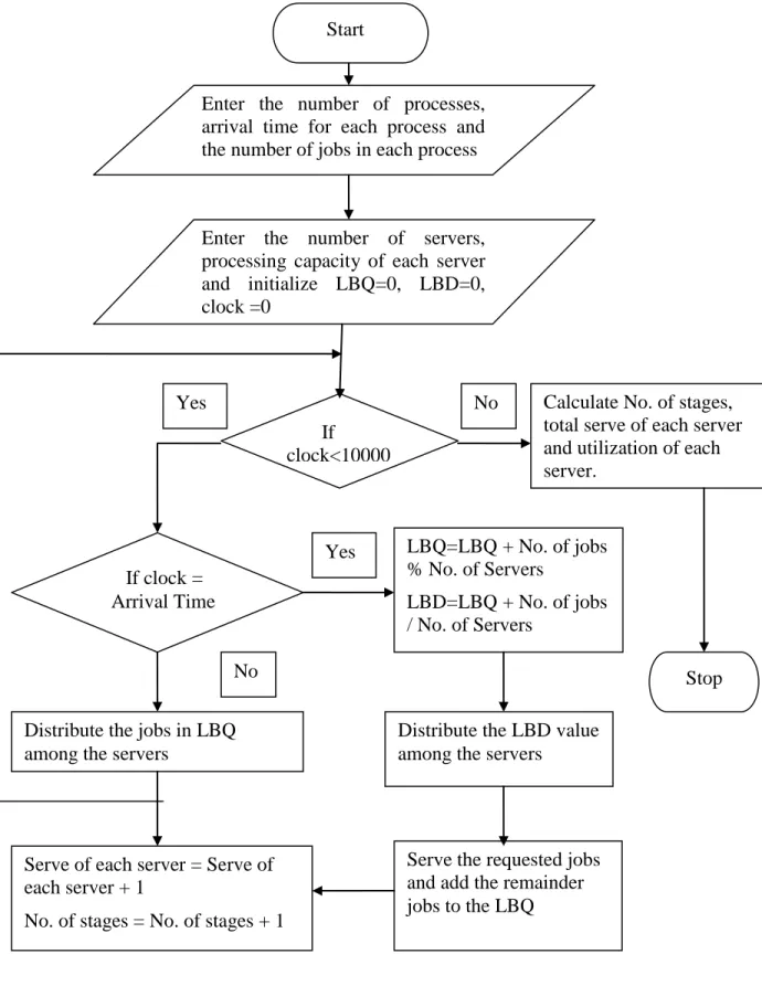
After the calculation of LBD and LBQ the traffic amount that is calculated from LBD is distributed among the servers. Each server will serve the requested traffic according to the number of jobs it can serve per unit of time. After this time the remainder jobs will be sent back to the network load balancer and will be added to the LBQ. By the end of the serve the number of stages is incremented by 1 and the number of serve for each server is incremented by 1. The block diagram of the proposed algorithm is shown in figure 5.1 below
Figure 5.1: Block diagram of the proposed algorithm 5.3: STEPS OF THE ALGORITHM
Step 1: Enter the number of processes, arrival time of each process and the number of jobs for each process.
Step 2: Specify the number of servers and the number of jobs they can serve per unit time. Initialize LBQ = 0, LBD = 0 and clock = 0.
Step 3: Repeat steps 4 to 6 till clock is less than 1000.
Step 4: If clock = arrival time
(i) LBQ = (LBQ + Number of Jobs) %Number of Servers.
(ii) LBD = (LBQ + Number of Jobs) /Number of Servers.
(iii) Distribute the LBD values among the servers. After one unit of time the remaining jobs at the servers are sent back to the LBQ. Else go to step 5.
Step 5: Check LBQ and distribute the available jobs to the servers.
Step 6: Serve for each server = Serve for each server + 1.
No. of stages = No. of stages + 1.
Step 7: Utilization of server= number of serves /number of stages.
5.4: FLOWCHART OF PROPOSED ALGORITHM
Figure 5.2 Flow chart of the proposed algorithm
Enter the number of processes, arrival time for each process and the number of jobs in each process
Distribute the jobs in LBQ among the servers
Enter the number of servers, processing capacity of each server and initialize LBQ=0, LBD=0, clock =0 If clock<10000 If clock = Arrival Time LBQ=LBQ + No. of jobs % No. of Servers LBD=LBQ + No. of jobs / No. of Servers
Distribute the LBD value among the servers
Serve the requested jobs and add the remainder jobs to the LBQ Serve of each server = Serve of
each server + 1
No. of stages = No. of stages + 1
Calculate No. of stages, total serve of each server and utilization of each server. Stop No Yes No Yes Start
5.5 PSEUDOCODE
READ nojob, tot, stage, no_job, res
INITIALIZE lbq=0, lbd=0, clock=0, rem=0 WHILE (clock<1000) IF (clock==1) IF(nojob[clock]<3) co=0 REPEAT tot[co]=tot[co] + 1 stage[co] = stage[co] + 1 UNTILL co>=2 lbq=0 ELSE lbd = (lbq+nojob[clock])/3 lbq = (lbq+nojob[clock])%3 co=0 REPEAT IF (lbd<=no_job[co] tot[co]=tot[co] + 1 stage[co] = stage[co] + 1 ELSE tot[co]=tot[co] + (no_job[co]) stage[co] = stage[co] + 1 rem=lbd- no_job[co] lbq=lbq+rem rem=0 ENDIF UNTILL co>=2 ENDIF ELSE IF(lbq>0) IF(lbq>3) lbd=lbq/3 lbq=lbq%3 co=0 REPEAT IF(lbd<=no_job[co]) tot[co]=tot[co] + lbd stage[co] = stage[co] + 1 ELSE tot[co]=tot[co] + (no_job[co]) stage[co] = stage[co] + 1 rem=lbd- no_job[co] lbq=lbq+rem rem=0
ENDIF UNTILL co>=2 ELSE IF(lbq= = 3) lbd=lbq/3 lbq=0 REPEAT IF(lbd<=no_job[co]) tot[co]=tot[co] + lbd stage[co] = stage[co] + 1 ELSE tot[co]=tot[co] + (no_job[co]) stage[co] = stage[co] + 1 rem=lbd- no_job[co] lbq=lbq+rem rem=0 ENDIF UNTILL co>=2 ENDIF ELSE IF(lbq<3) ilbq=0 WHILE(ilbq<3) IF(lbq= =1) tot[test] = tot[test] + 1 stage[test]=stage[test]+1 lbq=0 ELSEIF(lbq>1) tot[test] = tot[test] + 1 stage[test]=stage[test]+1 lbq=lbq-1 ENDIF test=(test+1)%3 ilbq=ilbq+1 ENDWHILE ENDIF clock =clock+1 ENDIF ELSE clock =clock+1 ENDIF ENDIF ENDWHILE
5.6: EXPERIMENTAL EVALUATION
In this work C#.net 2005 has been used for implementing the proposed algorithm. The algorithm has been checked for a number of inputs and results of five of them are shown here. Different values of the parameters have been taken to see the effect of each parameter on the algorithm
Experiment 1
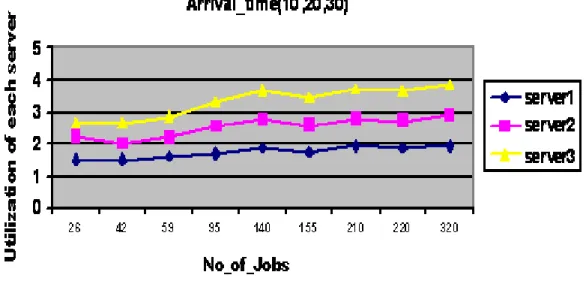
In this experiment the utilization of each server has been investigated by fixing the number of the jobs that each server can serve per unit time and changing the number of jobs of each process. The arrival time of each process was considered as given in table 5.1 with a time difference of 10 units
Process Number Arrival Time 1 10 2 20 3 30
Table 5.1: Arrival time of processes
Server Number No. of Jobs Served/Unit Time
1 2
2 3
3 4
Table 5.2: Number of jobs served by each server
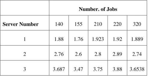
Table 5.3 shows the results of the experiment as utilization of different servers with changing load. The same result is also shown in the graphical form in figure 5.3
Number. of Jobs
Server Number 140 155 210 220 320 1 1.88 1.76 1.923 1.92 1.889 2 2.76 2.6 2.8 2.89 2.74 3 3.687 3.47 3.75 3.88 3.6538
Table 5.3: Utilization of different servers as the number of jobs varies
It has been noted that as the number of jobs increases the utilization of each server also increases proportionally. Because Server 3 can serve maximum number of the jobs per unit time so server 3 has best utilization. This is pictorially depicted in figure 5.3.
Figure 5.3:.The relation between utilization of each server and number of jobs Experiment 2
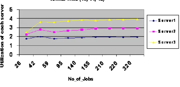
In this experiment the utilization of each server has been investigated when the processes are arriving at a constant time difference of one unit as shown in table 5.4
Process Number Arrival Time
1 10
2 11
3 12
Table 5.4: Arrival time of processes
Server Number No. of Jobs Served/Unit Time
1 2
2 3
3 4
Table 5.5: Number of jobs served by each server
It has again been noted that the utilization increases in proportion to the number of jobs served. Because Server 3 can serve maximum number of the jobs per unit time so server 3 has best utilization. This result has been shown graphically in figure 5.4.
Experiment 3
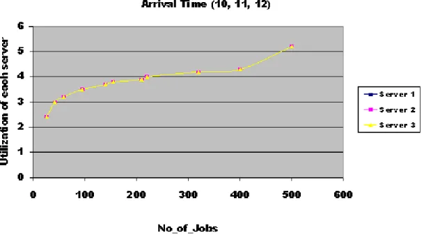
In this experiment it has been considered that all the servers are at par and hence can serve equal number of jobs per unit of time. This value has been taken to be equal to 2 jobs per unit time and arrival times of different processes are taken as 10, 11 and 12 respectively. Again it has been noted that the utilization increases with the increase in the number of jobs. In this experiment, as all the servers can serve same number of jobs per unit time so they all have same utilization. This result can be seen in figure 5.5.
Figure 5.5: The relation between utilization of each server and number of jobs Experiment 4
In this experiment the utilization of each server has been investigated by fixing the number of jobs for each process and changing the number of the jobs that each serve can
serve per unit time. The arrival time for each process and the number of jobs in each process has been considered as follows
Arrival time for process 1 =10 Arrival time for process 2=11 Arrival time for process 3=12 Number of jobs in process 1=52 Number of jobs in process 2=209 Number of jobs in process 3=159
Figure 5.6: The relation between utilization of each server and no. of jobs each server can serve.
As can be seen from figure 5.6 above the utilization is increasing proportionally with the increase in the number of jobs. This result has also been shown in tabular form in table 5.6 below.
S. No. No. of jobs that each server can serve
Utilization of each server 1 2 2 2 3 2.987 3 4 4 4 5 5 5 6 5.833 6 7 7 7 8 7.77 8 9 8.75 9 10 10 10 11 10.769
Table 5.6: Relationship between the number of jobs that a server can serve per unit time and the utilization.
Experiment 5
In this experiment the number of stages in which the load balancer is able to complete the total distribution and execution of processes is investigated. Here the number of jobs for each process is fixed and the serving capacity of each server changes. The arrival time of the processes were considered as follows
Arrival time for process 1 =10 Arrival time for process 2=11 Arrival time for process 3=12 Number of jobs in process 1=52 Number of jobs in process 2=209 Number of jobs in process 3=159
Figure 5.7: The relation between number of jobs each server can serve per unit time and number of stages
It was noted that the number of jobs that each server can serve per unit time is inversely proportional to the number of stages. This result can be seen in figure 5.7 above. The same results are also shown in table 5.7.
S. No. No of jobs that each server can serve per
unit of time Stages 1 2 70 2 3 47 3 4 35 4 5 28 5 6 24 6 7 20 7 8 18 8 9 16 9 10 14 10 11 13
Table 5.7: The relation between number of jobs each server can serve per unit time and number of stages
5.7 SUMMARY
In this chapter a new algorithm for load balancing has been discussed. Preliminary results show that this algorithm has the potential to significantly improve fairness of load balancing between the servers when ever the traffic is coming. The capacity of the server is of major importance in the serving of traffic request. The fairness is very important to increase the performance of the system as well as it gives out all the clients request in shortest time and help the system to be scalable.