DIFFRACTION FROM A SLIT IN AN IMPEDANCE PLANE PLACED AT THE INTERFACE OF TWO
SEMI-INFINITE HALF SPACES OF DIFFERENT MEDIA
A. Imran and Q. A. Naqvi
Department of Electronics Quaid-i-Azam University Islamabad 45320, Pakistan
K. Hongo
3-34-24, Nakashizu, Sakura City, Chiba, Japan
Abstract—Diffraction of an electromagnetic plane wave from a slit in an impedance plane placed at the interface of two different media, has been formulated rigorously. Both the principal polarizations are considered. The method of analysis is Kobayashi Potential (KP). To determine the unknown weighting functions, boundary conditions are imposed which resulted into dual integral equations (DIEs). These DIEs are solved by using the discontinuous properties of Weber-Schafheitlin’s integrals. The resulting expressions are then expanded in terms of Jacobi’s polynomials. The problems are then, reduced to matrix equations with infinite number of unknowns whose elements are expressed in terms of infinite integrals. These integrals are hard to solve analytically. The integrals contain poles for particular values of surface impedance and are solved numerically. Illustrative computations are given for far diffracted fields and other physical quantities of interest. To check the validity of our work, we compared the far field patterns with those of obtained through Physical Optics (PO). The agreement is good.
1. INTRODUCTION
properties of non perfectly electrically conducting (non-PEC) materials on diffraction phenomenon is an important and interesting. In the present study, we investigate the diffraction from a slit in an impedance plane placed at the interface of two semi-infinite half spaces of two different media and study how the surface impedance effects the diffracting properties of the slit. We have also included the effects of the media surrounding the slit in our study. Some interesting works on the topic are [3–5].
The method of analysis adopted here is the Kobayashi Potential (KP) method. This method uses the discontinuous properties of Weber-Schafheitlin integral. This integral is an infinite integral and its integrand consists of the product of two Bessel’s functions multiplied by the powered algebraic single term [15]. This integral shows a discontinuous property when a particular relation holds among the power of the algebraic term and orders of the Bessel’s functions. This method has been successfully applied to potential [6, 7] as well as scattering problems for different geometries [8–13]. Imposition of the boundary conditions result in dual integral equations (DIEs). These DIEs can be solved using the above properties of Weber-Schafheitlin integrals and projection method like the method of moment (MoM), in which Jacobi’s polynomials are used as the basis functions. One peculiarity of this method is that it provides the option to incorporate the edge conditions. Finally, the problem reduces to matrix equations whose matrix elements are the infinite integrals. These equations can be solved for the determination of unknown expansion coefficients. Numerical computations are conducted for the physical quantities of interest. We compared our results with those obtained through Physical Optics (PO) and found that these are in good agreement.
2. FORMULATION AND SOLUTION OF THE PROBLEM
2.1. E-polarization
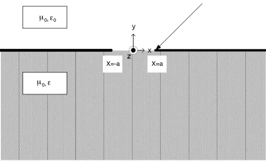
The configuration of the problem is shown in Fig. 1. Let the surface impedances of the upper and lower surfaces of the plane are Z+ and
Z−. We take0,µ0 as the constitutive parameters of the upper space
y >0and,µ0as the constitutive parameters of the lower spacey <0. The width of the slit is 2a. If φ0 is the angle of incidence, then Ezi,
µ 0,ε0
X=a X=-a
µ 0,ε
Figure 1. Geometry of the problem.
can be written as
Ezi = exp [jk0(xcosφ0+ysinφ0)] (1a)
Ezr = −Z0−Z+sinφ0
Z0+Z+sinφ0
exp [jk0(xcosφ0−ysinφ0)] (1b)
We assume the scattered fieldsEd+
z in the upper spacey >0andEd − z
in the lower space y <0in the form
Edz+ =
∞
0
{g1(ξ) cos (xaξ)
+g2(ξ) sin (xaξ)}exp
−ξ2−κ2
0ya
dξ y >0(1c)
Ezd− =
∞
0
{h1(ξ) cos (xaξ)
+h2(ξ) sin (xaξ)}exp
ξ2−κ2y
a
dξ y <0(1d)
where κ0 = k0a, κ = ka, xa = xa, ya = ya and k0, k are the propagation constant of the upper and lower space respectively. The
g1,2(ξ) andh1,2(ξ) are the weighting functions to be determined from the boundary conditions.
The required boundary conditions are given by
Ezt
y=0+
= −Z+Hxt y=0+
, Ezt
y=0− =Z−H
t x
y=0−; |xa| ≥1 (2a)
Ezt
y=0+
= Ezt
y=0−, H
t x
y=0+
=Hxt
where superscript tmeans total. From the condition (2a) we have
∞
0
1−j
ξ2−κ2 0
κ0
ζ+
[g1(ξ) cos(xaξ) +g2(ξ) sin(xaξ)]dξ= 0 ;
|xa| ≥1 (3a)
∞
0
1−j
ξ2−κ2
κ ζ−
[h1(ξ) cos(xaξ) +h2(ξ) sin(xaξ)]dξ= 0 ;
|xa| ≥1 (3b)
whereζ+ and ζ− are the normalized surface impedances of the plane. And from the boundary conditions (2b), we have
∞
0
{[h1(ξ)−g1(ξ)] cos(xaξ) + [h2(ξ)−g2(ξ)] sin(xaξ)}dξ
= 2ζ+sinφ0 1 +ζ+sinφ0
exp[jκ0xacosφ0] (3c)
∞
0
ξ2−κ2h 1(ξ) +
ξ2−κ2 0g1(ξ)
cos(xaξ)
+ξ2−κ2h 2(ξ) +
ξ2−κ2 0g2(ξ)
sin(xaξ)
dξ
= j2κ0sinφ0 1 +ζ+sinφ0
exp[jκ0xacosφ0] |xa| ≥1 (3d)
The above expressions are the dual integral equations. Making using of the discontinuous properties of Weber-Schafheitlin’s integrals and the edge conditions of E-field, we can decide the nature of weighting functionsg1,2(ξ) and h1,2(ξ) as follow
g1(ξ) =
1
jκ0η++
ξ2−κ2 0
∞
m=0
AmJ2m+3 2(ξ)ξ
−3 2,
g2(ξ) =
1
jκ0η++
ξ2−κ2 0
∞
m=0
BmJ2m+5 2(ξ)ξ
−3 2
(4a)
h1(ξ) =
1
jκη−+ξ2−κ2
∞
m=0
CmJ2m+3 2(ξ)ξ
−3 2,
h2(ξ) =
1
jκη−+ξ2−κ2
∞
m=0
DmJ2m+5 2(ξ)ξ
−3 2
where η± = ζ±−1 and Jm(.) be the Bessel’s function of order m. The
above solutions for the functions g1,2(ξ) and h1,2(ξ) signify that the tangential components of electromagnetic field are finite at the edge. Separating even and odd functions of the expressions (3c) and (3d) and then projecting the resulting equations into the functional space
with elements p±
1 2
n (x2a) [14], we obtain the matrix equations for the
expansion coefficients
∞
m=0
−AmGSE
2m+3
2,2n+ 1 2;κ
+ 0
+CmGSE
2m+3
2,2n+ 1 2;κ
−
= 2ζ+sinφ0 1 +ζ+sinφ0
J2n+1
2(κ0cosφ0)
(κ0cosφ0)
1 2 (5a) ∞ m=0
−BmGSE
2m+5
2,2n+ 3 2;κ
+ 0
+DmGSE
2m+5
2,2n+ 3 2;κ
−
= j2ζ+sinφ0 1 +ζ+sinφ0
J2n+3
2(κ0cosφ0)
(κ0cosφ0)
1 2 (5b) ∞ m=0
AmKSE
2m+3
2,2n+ 1 2;κ
+ 0
+CmKSE
2m+3
2,2n+ 1 2;κ
−
= j2κ0sinφ0 1 +ζ+sinφ0
J2n+1
2(κ0cosφ0)
(κ0cosφ0)
1 2 (5c) ∞ m=0
BmKSE
2m+5
2,2n+ 3 2;κ
+ 0
+DmKSE
2m+5
2,2n+ 3 2;κ
−
=− 2κ0sinφ0 1 +ζ+sinφ0
J2n+3
2(κ0cosφ0)
(κ0cosφ0)
1 2
n= 0,1,2, . . . (5d)
where GSE µ, ν;κ±= ∞ 0 1
jκη±+ξ2−κ2
Jµ(ξ)Jν(ξ)
ξ dξ (6a)
KSE µ, ν;κ±= ∞ 0
ξ2−κ2
jκη±+ξ2−κ2
Jν(ξ)Jν(ξ)
In writing the Equation (5), we have used the following relations
cosx=
πx
2 J−12(x) (7a)
sinx=
πx
2 J12(x) (7b)
x−m/2Jm
ξ√x =
∞
n=0
2(2n+m+1)Γ(n+m+1) Γ(n+ 1)Γ(m+ 1)
J2n+m+1(ξ)
ξ p
m n(x)(7c)
pmn(x) = Γ(n+ 1)Γ(m+ 1) Γ (n+m+ 1) x
−m/2
∞
0
Jm( √
xξ)J2n+m+1(ξ)dξ (7d)
wherepmn(x) be the Jacobi’s polynomials [14].
The Equation (5) are the matrix equations and we write them in matrix notation as under
−G+SE,E
[Am] +
G−SE,E
[Cm] =ζ+[JE],
KSE,E+
[Am] +
KSE,E−
[Cm] =jκ0[JE]
(8a)
−G+SE,O
[Bm] +
G−SE,O
[Dm] =jζ+[JO],
KSE,O+
[Bm] +
KSE,O−
[Dm] =−κ0[JO]
(8b)
where the correspondence between the matrices and their elements are given by
G±SE,E
⇐⇒GSE
2n+1
2,2m+ 3 2;ζ±
,
G±SE,O
⇐⇒GSE
2n+3
2,2m+ 5 2;ζ±
KSE,E±
⇐⇒KSE
2n+1
2,2m+ 3 2;ζ±
,
KSE,O±
⇐⇒KSE
2n+3
2,2m+ 5 2;ζ±
[JE]⇐⇒
2 sinφ0 1 +ζ+sinφ0
J2n+1
2(κcosφ0)
(κcosφ0)
1 2
,
[JO] ⇐⇒
2 sinφ0 1 +ζ+sinφ0
J2n+3
2(κcosφ0)
(κcosφ0)
1 2
Equation (8) can be solved for the expansion coefficientsAm,Bm,Cm,
Dm as follow
G+SE,E
−1
G−SE,E
+
KSE,E+
−1
KSE,E−
[Cm]
=
ζ+
G+SE,E
−1 +jκ0
KSE,E+
−1
[JE] (10a)
[Am] =
G+SE,E
−1
G−SE,E
[Cm]−ζ+
G+SE,E
−1
[JE] (10b)
G+SE,O
−1
G−SE,O
+
KSE,O+
−1
KSE,O−
[Dm]
=
jζ+
G+SE,O
−1
−κ0
KSE,O+
−1
[JO] (10c)
[Bm] =
G+SE,O
−1
G−SE,O
[Dm]−jζ+
G+SE,O
−1
[JO] (10d)
The geometry supports the surface wave. When the observation point is far from the surface, these waves can be neglected and diffracted waves dominates. A far diffracted fields in the upper region can be evaluated by applying the saddle point method of integration. The result is given by
Ezd =
∞ m=0 ∞ 0 jκ0
jκ0+
ξ2−κ2 0ζ+
Am
J2m+3 2(ξ)
ξ32
cos(xaξ)
+Bm
J2m+5 2(ξ)
ξ32
sin(xaξ)
exp
−ξ2−κ2
0ya dξ = π 2 tanφ
1 +ζ+sinφ 1
√
k0ρ exp
−jk0ρ+j
π 4 ∞ m=0 Am
J2m+3
2(κ0cosφ) √
κ0cosφ
+jBm
J2m+5
2(κ0cosφ) √
κ0cosφ
(11)
2.2. H-polarization
The field expressions corresponding to expressions (1) for H -polarization may be written as
Hzi = exp [jk0(xcosφ0+ysinφ0)] (12a)
Hzr = −Z++Z0sinφ0
Z++Z0sinφ0
exp [jk0(xcosφ0−ysinφ0)] (12b)
Hzd+ =
∞
0
{g1(ξ) cos (xaξ) +g2(ξ) sin (xaξ)}
exp
−ξ2−κ2
0ya
dξ y >0(12c)
Hzd− =
∞
0 {
h1(ξ) cos (xaξ) +h2(ξ) sin (xaξ)}
expξ2−κ2y
a
dξ y <0(12d)
All the notations used in the above expressions have the same meaning as described in last section.
The boundary conditions are
Ext
y=0+
= Z+Hzt y=0+
, Ext
y=0− =−Z−H
t z
y=0−; |xa| ≥1 (13a)
Ext
y=0+
= Ext
y=0−, H
t z
y=0+
=Hzt
y=0−; |xa| ≤1 (13b)
Using (13a), we get
∞
0
[u+jκ0ζ+] [g1(ξ) cos(xaξ) +g2(ξ) sin(xaξ)]dξ= 0 ; |xa| ≥1(14a)
∞
0
[v+jκζ−] [h1(ξ) cos(xaξ) +h2(ξ) sin(xaξ)]dξ= 0 ; |xa| ≥1(14b)
where u = ξ2−κ2 0, v =
ξ2−κ2 and ζ
+, ζ− are the normalized impedances of upper and lower surface of the impedance plane respectively.
Using the discontinuous properties of Weber-Schafheitlin’s integrals and incorporating the edge conditions forH-field, we get
g1(ξ) = 1
jκ0ζ++u
∞
m=0
AmJ2m+1 2(ξ)ξ
−1 2,
g2(ξ) = 1
jκ0ζ++u
∞
m=0
BmJ2m+3 2(ξ)ξ
−1 2
h1(ξ) = 1
jκζ−+v ∞
m=0
CmJ2m+1 2(ξ)ξ
−1 2,
h2(ξ) = 1
jκζ−+v ∞
m=0
DmJ2m+3 2(ξ)ξ
−1 2 (15b) From (13b) ∞ 0 {
[g1(ξ)−h1(ξ)] cos(xaξ) + [g2(ξ)−h2(ξ)] sin(xaξ)}dξ
= 2 sinφ0
ζ++ sinφ0
exp[jκ0xacosφ0] (16a)
∞
0
{[vh1(ξ) +rug1(ξ)] cos(xaξ)+[vh2(ξ)+rug2(ξ)] sin(xaξ)}dξ
= j2κ0ζ+sinφ0
ζ++ sinφ0
exp[jκ0xacosφ0] |xa| ≥1 (16b)
Proceeding in a similar manner as in last section, we get the matrix equations
∞
m=0
AmGSH
2m+1
2,2n+ 1 2;κ
+ 0
−CmGSH
2m+1
2,2n+ 1 2;κ
−
= 2 sinφ0
ζ++ sinφ0
J2n+1
2(κ0cosφ0)
(κ0cosφ0)
1 2 (17a) ∞ m=0
BmGSH
2m+3
2,2n+ 3 2;κ
+ 0
−DmGSH
2m+3
2,2n+ 3 2;κ
−
= j2 sinφ0
ζ++ sinφ0
J2n+3
2(κ0cosφ0)
(κ0cosφ0)
1 2 (17b) ∞ m=0
AmKSH
2m+1
2,2n+ 1 2;κ
+ 0
+CmKSH
2m+1
2,2n+ 1 2;κ
−
= j2κ0ζ+sinφ0
ζ++ sinφ0
J2n+1
2(κ0cosφ0)
(κ0cosφ0)
1 2 (17c) ∞ m=0
BmKSH
2m+3
2,2n+ 3 2;κ
+ 0
+DmKSH
2m+3
2,2n+ 3 2;κ
−
= −2κ0ζ+sinφ0
ζ++ sinφ0
J2n+3
2(κ0cosφ0)
(κ0cosφ0)
1 2
where
GSH
µ, ν;κ± =
∞
0
1
jκζ±+ξ2−κ2
Jµ(ξ)Jν(ξ)
ξ dξ (18a)
KSH
µ, ν;κ± =
∞
0
r
ξ2−κ2
jκζ±+ξ2−κ2
Jµ(ξ)Jν(ξ)
ξ dξ (18b)
The above expressions are the matrix equations and can be solved for the expansion coefficientsAm,Bm,Cm,Dm by any standard method.
The geometry supports the surface waves but if we use the asymptotic analysis, we can ignore the contribution of these waves. So applying the saddle point method, far diffracted fields in the upper space may be written as
Hzd+ =
π
2
sinφ ζ++ sinφ
1
√
k0ρ exp
−jk0ρ+j
π
4
∞
m=0
Am
J2m+1
2(κ0cosφ) √
κ0cosφ
+jBm
J2m+3
2(κ0cosφ) √
κ0cosφ
(19)
where (ρ = x2
a+ya2, φ) are the coordinates of observation point in
cylindrical coordinates.
-20 0 20 40 60 80 100 120 140 160 180 200 -1
0 1 2 3 4 5 6 7 8 9 10
DIFFRACTED FIELD
OBSERVATION ANGLE φ0=60
φ0=90 κ0=6.0 κ=8.0 ζ± =0.2−0.5
-20 0 20 40 60 80 100 120 140 160 180 200 0
2 4 6 8
DIFFRACTED FIELD
OBSERVATION ANGLE KP
PO φ0=90 κ=4.0 κ0=4.0 ζ±=0.2−0.5i
E-POLARIZATION
Figure 3. Comparison of the patterns obtained through KP and PO.
-20 0 20 40 60 80 100 120 140 160 180 200 -2
0 2 4 6 8 10 12 14
DIFFRACTED FIELD
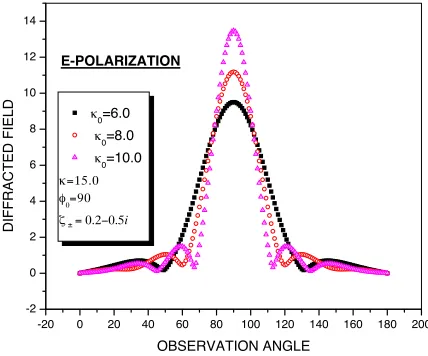
OBSERVATION ANGLE κ0=6.0
κ0=8.0 κ0=10.0 κ=15.0 φ0=90 ζ = 0.2−0.5± i
E-POLARIZATION
Figure 4. Effect of slit width on the field patterns.
3. RESULTS AND DISCUSSIONS
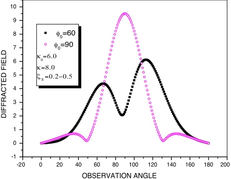
The field patterns are computed from Equation (11) forE-polarization and Equation (19) for H-polarization. But these equations contain the unknowns expansion coefficients Am,Bm,Cm,Dm. The values of
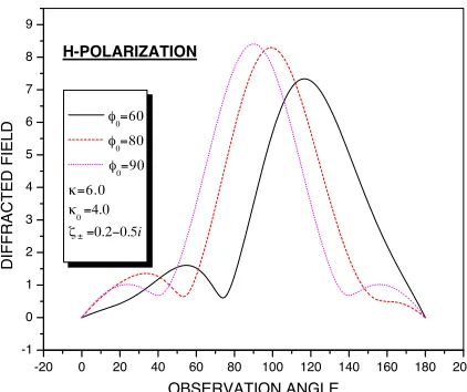
taken the matrix size (2κ0 + 3) × (2κ0 + 3) in our computations. The far field patterns are shown in Fig. 2 and Fig. 6 for E- and H -polarizations respectively for different angle of incidence. We notice that the peak of the main lobe corresponding to an angle of incidence occurs approximately at π−φ0 and as we increaseφ0, the main lobe shifts towards the lower value of φ. To verify the validity of our
-20 0 20 40 60 80 100 120 140 160 180 200 -2
0 2 4 6 8 10 12 14 16
DIFFRACTED FIELD
OBSERVATION ANGLE κ0=6.0
κ=8.0 φ0=90
E-POLARIZATION
ζ = 0.2−0.5± i ζ = 0.2−0.7± i ζ = 0.2−0.9± i
Figure 5. Diffracted patterns for different values of impedance of plane.
-20 0 20 40 60 80 100 120 140 160 180 200 -1
0 1 2 3 4 5 6 7 8 9
DIFFRACTED FIELD
OBSERVATION ANGLE φ0=60
φ0=80 φ0=90 κ=6.0 κ =4.00
H-POLARIZATION
ζ =0.2−0.5± i
computations, we have compared our results with those of obtained through Physical Optics (PO). The comparison for E-polarization is given in Fig. 3. The angle of incidence φ0 is π2 and the surface impedances are chosen as ζ± = 0.2−0.5i. Similarly Fig. 7 shows the comparison for H-polarization. All the parameters are same except
φ0, which is π3 in this case. The comparison is fairly good for both the cases. Fig. 4 and Fig. 8 give the variations in the field patterns
-20 0 20 40 60 80 100 120 140 160 180 200 0
1 2 3 4 5
DIFFRACTED FIELD
OBSERVATION ANGLE KP
PO φ0=60 κ=4.0 κ0=4.0
H-POLARIZATION
ζ =0.2−0.5± i
Figure 7. Comparison of the two methods for H-polarization.
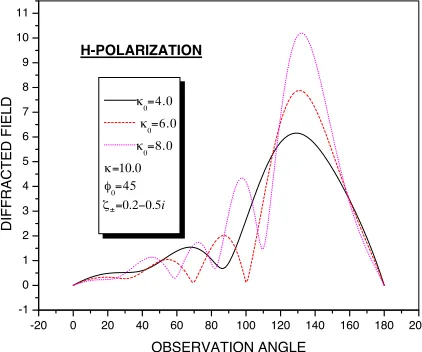
-20 0 20 40 60 80 100 120 140 160 180 200 -1
0 1 2 3 4 5 6 7 8 9 10 11
DIFFRACTED FIELD
OBSERVATION ANGLE κ0=4.0
κ0=6.0 κ0=8.0 κ=10.0 φ0=45
H-POLARIZATION
ζ =0.2−0.5± i
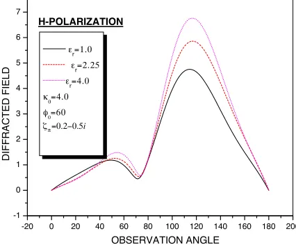
as we increase the slit width. Fig. 5 is intended to show the effects of material properties of the plane on the diffracted fields. It gives, as we decrease the impedances of the plane, the strength of the field patterns intensifies. We also computed the far field patterns to see the effects of medium properties of lower space. Fig. 9 presents the same. The field patterns are given forr= 1.0, r= 2.25, and r = 4.0 . We
choose the other parameters asφ0= π3,ζ±= 0.2−0.5i. It shows that as we increase the value of r, the strength of the diffracted fields in
the upper space (y >0) also increase.
-20 0 20 40 60 80 100 120 140 160 180 200 -1
0 1 2 3 4 5 6 7
DIFFRACTED FIELD
OBSERVATION ANGLE εr=1.0
εr=2.25 εr=4.0 κ0=4.0 φ0=60
H-POLARIZATION
ζ =0.2−0.5± i
Figure 9. Effects of medium materials on the scattered fields.
APPENDIX A. HOW TO COMPUTE THE INTEGRALS GSE(µ, ν, κ±),KSE(µ, ν, κ±), GSH(µ, ν, κ±) and KSH(µ, ν, κ±)
First we take the integral
GSE(µ, ν;κ±) =
∞
0
1
jκη±+ξ2−κ2
Jµ(ξ)Jν(ξ)
ξ dξ
= x
0
1
jκη±+ξ2−κ2
Jµ(ξ)Jν(ξ)
ξ dξ
+
∞
x
1
jκη±+ξ2−κ2
Jµ(ξ)Jν(ξ)
ξ dξ
where x is a fairly large constant and we chose x = 300 in our computation. The integral GxSE(µ, ν;κ±) may be evaluated easily
by using the definition of Spherical Bessel Function [17] since µ, ν are the half order numbers. And these functions are convergent [17] and so is the integral GxSE(µ, ν;κ±). The second integralG∞SE(µ, ν;κ±)
can be computed as follow
G∞SE(µ, ν;κ±) =
∞
x
1
jκη±+ξ2−κ2
Jµ(ξ)Jν(ξ)
ξ dξ
∞
x
Jµ(ξ)Jν(ξ)
ξ2 −jκη±
∞
x
Jµ(ξ)Jν(ξ)
ξ3 dξ
+κ 2
2
∞
x
Jµ(ξ)Jν(ξ)
ξ4 dξ (A1b)
To perform the above numerical integrations, we need to have the Hankel approximation of the Bessel function. That is given by
Jn(ξ)=
2
πξ
1−(4n
2−1)(4n2−9)
128ξ2
+(4n
2−1)(4n2−9)(4n2−25)(4n2−49)
98304ξ4
cos
ξ− 2n+ 1
4 π
−
(4n2−1) 8ξ −
(4n2−1)(4n2−9)(4n2−25) 3072ξ3
sin
ξ−2n+ 1
4 π
(A2)
Using this formula we may write
Jm(ξ)Js(ξ) =
1
π
1
ξ −
a2+b2−a1b1
ξ3
+a4+b4+a2b2−a1b3−b1a3
ξ5
cos(m−s)π 2
+1
π
a1−b1
ξ2 −
a1b2+a3−(a2b1+b3)
ξ4
sin(m−s)π 2
+1
π
1
ξ −
a2+b2+a1b1
ξ3
cos
2ξ−m+s+ 1
2 π
−1
π
a1+b1
ξ2 −
a1b2+a3+(a2b1+b3)
ξ4
sin
2ξ−m+s+1
2 π
a1 =
4m2−1
8 , a2 =
(4m2−1)(4m2−9)
128 ,
a3 =
a4 =
(4m2−1)(4m2−9)(4m2−25)(4m2−49) 98304
b1 =
4s2−1
8 , b2 =
(4s2−1)(4s2−9)
128 ,
b3 =
(4s2−1)(4s2−9)(4s2−25) 3072
b4 =
(4s2−1)(4s2−9)(4s2−25)(4s2−49)
98304 (A3)
Integrating by parts and If we retain the terms up to ξ−5 with constant coefficients and ξ−4 multiplied by trigonometric functions. Then we can write
∞
x
Jµ(ξ)Jν(ξ)
ξ dξ =
1 π −1 x + A1 3x3
cosµ−ν 2 π
+
−A3
2x2 +
A5 4x4
sinµ−ν 2 π
+
1 2x2 −
A2 2x4 +
3A4 4x4 −
3 4x4
sin(2x−β)
+
− 1
2x3 + 3 2x5 +
A2
x5 +
A4 2x3 −
3A4 2x5
×cos(2x−β)]1
π (A4a)
∞
x
Jµ(ξ)Jν(ξ)
ξ2 dξ = 1
π
− 1
2x2 +
A1 4x4
cosµ−ν 2 π
+
1 2x3 −
3 2x5 +
A4
x5 −
A2 2x5
sin(2x−β)
+
− 3
4x4 +
A4 2x4
cos(2x−β)
+
−A3
3x3 +
A5 5x5
sin µ−ν 2 π (A4b) ∞ x
Jµ(ξ)Jν(ξ)
ξ3 dξ = 1
π
− 1
3x3 +
A1 5x5
cosµ−ν 2 π
+ 1
2x4 sin(2x−β) +
1
x5 +
A4 2x5
cos(2x−β)
−A3
4x4sin
µ−ν
2 π
∞
x
Jµ(ξ)Jν(ξ)
ξ4 dξ = 1
π
− 1
4x4cos
µ−ν
2 π
+ 1
2x5sin(2x−β)
−A3
5x5sin
µ−ν
2 π
(A4d)
where
A1 =
a2+b2−a1b1
ξ3 , A2=
a2+b2+a1b1
ξ3 , A3 =
a1−b1
ξ2
A4 =
a1+b1
ξ2 , A5 =
a1b2+a3−(a2b1+b3)
ξ4
Using the expressions (A4a)–(A4d), we can compute the integral
GSE(µ, ν;κ±) from (A1a). Similarly we can compute the remaining
integrals from the expressions
KSE
µ, ν;κ±=
∞
0
ξ2−κ2
jκη±+ξ2−κ2
Jµ(ξ)Jν(ξ)
ξ dξ
=−jκη±GSE
µ, ν;κ±+
∞
0
Jµ(ξ)Jν(ξ)
ξ dξ (A5)
GSH
µ, ν;κ± =
∞
0
1
jκζ±+ξ2−κ2
Jµ(ξ)Jν(ξ)
ξ dξ
= x
0
1
jκζ±+ξ2−κ2
Jµ(ξ)Jν(ξ)
ξ dξ
+
∞
x
Jµ(ξ)Jν(ξ)
ξ2 dξ+P1 x
0
Jµ(ξ)Jν(ξ)
ξ3 dξ
+P2
∞
x
Jµ(ξ)Jν(ξ)
ξ4 dξ (A6)
whereP1=−jκζ±,P2= (12 −ζ±2)κ2.
KSH
µ, ν;κ± =
∞
0
ξ2−κ2
jκζ±+ξ2−κ2
Jµ(ξ)Jν(ξ)
ξ dξ
= −jκζ±GSH
µ, ν;κ±+ 1
m+nδµ,ν (A7)
The same comments on the convergence for the case GxSE(µ, ν;κ±)
REFERENCES
1. Ziolkowski, R. W. and N. Engheta, Special Issue on “Metatama-terials,”IEEE Trans. Antennas and Propagation, Vol. 51, No. 10, Oct. 2003.
2. Munk, B. A., Frequency Selective Surfaces: Theory and Design, John Wiley, 2000.
3. Hongo, K., “Diffraction of electromagnetic plane wave by a slit,”
Trans. Inst. Electronics and Comm. Engrg. in Japan, Vol. 55-B,
No. 6, 328–330, 1972.
4. Hurd, R. A. and Y. Hayashi, “Low frequency scattering by a slit in a conducting plane,” Radio Sci., Vol. 15, 1171–1178, 1980. 5. Illahi, A., Q. A. Naqvi, and K. Hongo, “Scattering of dipole
field by a finite and a finite impedance cylinder,” Progress In
Electromagnetics Research M, Vol. 1, 139–184, 2008.
6. Kobayashi, I., “Darstellung eines potentials in zylindrischen koordinaten, das sich auf einer ebene innerhalb und ausserhalb einer gewissen kreisbegrenzung verschiedener grenzbedingung unterwirft,”Sci. Rep. Tohoku Univ., Ser. 1/20, 197–212, 1931. 7. Sneddon, I. N., Mixed Boundary Value Problems in Potential
Theory, North-Holland, Amsterdam, 1966.
8. Hongo, K. and H. Serizawa, “Diffraction of electromagnetic plane wave by a rectangular plate and a rectangular hole in the conducting plate,” IEEE Trans. on Antennas and Propagation, Vol. 47, No. 6, 1029–1041, June 1999.
9. Imran, A., Q. A. Naqvi, and K. Hongo, “Diffraction of plane wave by two parallel slits in an infinitely long impedance plane using the method of kobayashi potential,”Progress In Electromagnetics
Research, PIER 63, 107–123, 2006.
10. Hongo, K. and Q. A. Naqvi, “Diffraction of electromagnetic wave by disk and circular hole in a perfectly conducting plane,”Progress
In Electromagnetics Research, PIER 68, 113–150, 2007.
11. Serizawa, H. and K. Hongo, “Radiations from a flanged rectan-gular waveguidee,” IEEE Tran. on Antennas and Propagation, Vol. 53, No. 12, 3953–3962, Dec. 2005.
12. Imran, A., Q. A. Naqvi, and K. Hongo, “Diffraction of electro-magnetic plane wave by an strip,” Progress In Electromagnetics
Research, PIER 75, 303–318, 2007.
14. Magnus, W., F. Oberhettinger, and R. P. Soni, Formulas and
Theorems for the Special Functions of Mathematical Physics,
Spinger-Verlag, New York, 1966.