Vol. 11, No. 2, pp 173-190
Integer Valued AR(1) with Geometric
Innovations
Mansour Aghababaei Jazi1, Geoff Jones2, Chin-Diew Lai2
1Faculty of Mathematics, University of Sistan and Baluchestan, Zahedan, Iran. 2Institute of Fundamental Sciences, Massey University, Palmerston North, New Zealand.
Abstract. The classical integer valued first-order autoregressive (INA-R(1)) model has been defined on the basis of Poisson innovations. This model has Poisson marginal distribution and is suitable for modeling equidispersed count data. In this paper, we introduce an modification of the INAR(1) model with geometric innovations (INARG(1)) for model-ing overdispersed count data. We discuss some structural mathematical properties of the process comparing with classical INAR(1). Also, the superiority of the model in contrast with the INAR(1) is shown by some real time series.
Keywords. Binomial thinning operator, conditional maximum likeli-hood estimation, infinitely divisible distributions, mixture distributions. MSC: 62M10.
1
Introduction
Recently there has been growing interest in modeling discrete-time de-pendent integer valued time series. In developing such models the integer valued first-order autoregressive (INAR(1)) process, introduced indepen-dently by McKenzie (1985) and Al-Osh and Alzaid (1987), has received Mansour Aghababaei Jazi( )([email protected]), Geoff Jones (G.Jones @massey.ac.nz), Chin Diew Lai ([email protected])
Received: January 1, 2012; Accepted: May 14, 2012
considerable attention. This model has been defined on the basis of binomial thinning operator ◦of Steutel and van Harn (1979).
Definition 1.1. LetX be a nonnegative integer valued random vari-able (r.v.). Then for any α∈[0,1] the operator ◦is defined by
α◦X=
X ∑ i=1
Bi(α), (1)
where counting series Bi(α) is a sequence of independent identically
distributed (iid) binary r.v.’s with P(Bi(α) = 1) = 1−P(Bi(α) = 0) =
α.
Definition 1.2. A discrete-time dependent integer valued time series {Xt} is said to follow an INAR(1) model, if
Xt=α◦Xt−1+Wt, t= 0,1,2, ..., (2)
where{Wt} are iid nonnegative integer valued r.v.’s with some discrete
distribution and independent of all the counting seriesBi(α)’s in (1) and
Xt−1.
Note that α ∈ (0,1) implies a stationary dependent integer val-ued time series, whereas α = 0 and α = 1 imply independence and non-stationarity for Xt, respectively. The process Xt satisfying (2) is
second-order stationary if 0 ≤ α < 1, with autocovariance function Cov(Xt, Xt−k) =σ2αk (Al-Osh and Alzaid, 1987; Du and Li, 1991).
The coefficientαcan be interpreted as the proportion of observations counted at time t−1 that still remains at time t. Wt is known as the
innovations (or repositions) produced at time t and α ◦Xt−1 can be interpreted as the number of survivors at timetfrom the previous period. The INAR(1) process as defined by (2) can be viewed as both a Markov process and a GaltonWatson branching process with immigration.
Al-Osh and Alzaid (1987) provide the following representation for the marginal distribution of the INAR(1) model expressed in terms of the innovation sequenceWt,
Xt=
∞ ∑ i=0
αi◦Wt−i . (3)
The above representation implies that the marginal distribution of a stationary INAR(1) process is discrete self-decomposable, i.e., the prob-ability generating function (pgf) ofXt, denoted by ϕX(s), satisfies
ϕX(s) =ϕX(1−α+αs)ϕw(s) (4)
where ϕw is the pgf of innovations Wt. In fact, assuming that the
INAR(1) process is stationary, the pgf of Xt satisfies (4). Thus, one
can choose any member of the class of discrete self-decomposable dis-tributions as the marginal distribution of a stationary INAR(1) model. It is known that discrete self-decomposability implies infinite divisibility and unimodality (see Steutel and Van Harn, 2004). Subsequently, the stationary marginal distribution of a stationary INAR(1) is infinitely divisible and unimodal. Further, a stationary INAR(1) process has a Poisson marginal distribution (with mean θ) if and only if the inno-vations also follow a Poisson distribution (with mean (1−α)θ). So, INAR(1) with Poisson innovations is a suitable model for equidispersed count data wherein the mean and variance are the same. For more structural and asymptotic properties in INAR(1) process with Poisson marginal, we refer the reader to Silva and Oliveira (2004), Pavlopoulos and Karlis (2006) and Park and Oh(1997).
Autoregressive moving-average processes with Poisson marginal dis-tribution are appropriate for equidispersed time series of counts (where the mean is the same as the variance). In practice, however, some discrete time dependence count data may be overdispersed, i.e., the variance is greater than the mean. McKenzie (1986) developed autore-gressive moving-average processes with negative binomial and geomet-ric marginal distributions as analogues of well-known continuous vari-ates models for gamma and negative exponential varivari-ates. Also, Alzaid and Al-Osh (1988) considered INAR(1) processes (2) with geometric marginal distribution for time series of overdispersed counts. They de-noted the model by GINAR(1) and showed that the innovations are distributed as a mixture of a degenerated distribution at zero with mass α and a geometric distribution with mass 1−α.
Time series of overdispersed counts can also be modeled through overdispersed innovations. Let µw and σ2w be the mean and variance of
the innovations, then the mean and variance of the stationary solution of INAR(1) model (2) are
µ=E(Xt) =
µw
1−α and σ
2 =V ar(X
t) =
αµw+σw2
1−α2 ,
respectively. Thus, the index of dispersion of the solution, ID(X) = σ2/µ, is related to that of the innovations, ID(W) =σ2w/µw, according
to the formula
ID(X) = [1 +ID(W)/α]/[1 + 1/α].
showing that the marginal distribution of the solution {Xt} is
overdis-persed (i.e.,σ2> µ) if and only if the distribution of the innovations{Wt}
is overdispersed too (i.e., σ2w > µw). Also, for any fixed value of α,
ID(X) increases whenID(W) does, which in turn implies that in order for INAR(1) to be a suitable model for a series of counts with arbitrary large (sample) ID(X), the distribution of innovations must necessarily be such as to allow for quite large values ofID(W) too, in a rather flex-ible way. In light of this reasoning, e.g., Pavlopoulos and Karlis (2008) considered INAR(1) process (2) with innovations from finite mixtures of Poisson distributions.
In this paper, we study the INAR(1) process (2) with geometric innovations, denoted by INARG(1). The motivation for such a process arises from its potential in the modeling of some overdispersed integer-valued time series.
We also suppose here that a geometric r.v. (innovation) W, denoted by W ∼Ge(π), has probability mass function (pmf)
P(W =k) =π(1−π)kI{0,1,...}(k), (5)
where π ∈(0,1) and the indicator function IA(x) equals to 1, if x ∈A
else equals to zero. Also, the pgf of W is given by ϕw(s) =
π 1−(1−π)s
It is easy to show that the mean and the variance of W with the pmf (5) are µw = (1−π)/π and σw2 = (1−π)/π2, respectively, with
ID(W) = 1/π >1.
The contents of this paper are organized as follows. Some mathe-matical and structural properties of the INARG(1) process are derived in Section 2. In Section 3, we discuss parameter estimation and fore-casting for our models. In Section 4, we use simulation to study the marginal distribution of INARG(1) process and comparing two maxi-mum likelihood based estimation approaches. Finally, in Section 5, we fit both Poisson INAR(1) and INARG(1) models on some real time se-ries to show the superiority of the INARG(1) model over the traditional INAR(1) with Poisson innovations.
2
INAR(1) With Geometric Innovations
In this section we introduce an INAR(1) process with geometric inno-vations and derive some mathematical and structural properties of the
corresponding marginal distribution of the process, e.g., the mean, vari-ance, autocovariance and (conditional) likelihood functions. Also, we compare the average run length of zeros and proportions of zeros in the INARG(1) process and classic INAR(1) process with Poisson innova-tions to derive a simple check on the distribution of innovainnova-tions in the INAR(1) processes.
We modify classic INAR(1) model of McKenzie (1985) and Al-Osh and Alzaid (1987) and Alzaid and Al-Osh(1988) as follow.
Definition 2.1. {Xt} is said to follow a INAR(1) process with
geo-metric innovation, denoted by INARG(1), if
Xt=α◦Xt−1+Wt, t= 0,1,2, ..., (6)
where {Wt}are iid Ge(π) r.v.’s independent of Xt−1 and operator◦ as defined in (1).
2.1 Some Mathematical Properties
In the following theorems, suppose that{Xt} follow an INARG(1)
pro-cess (6) with Ge(π) innovations.
Theorem 2.1. The mean and variance of Xt are
µ= 1−π
π(1−α) (7)
and
σ2 = 1−π
π2(1−α), (8)
respectively.
Proof. We have
E[Xt|Xt−1] = E[α◦Xt−1+Wt|Xt−1]
= E[α◦Xt−1|Xt−1] +E[Wt|Xt−1]
= αXt−1+ (1−π)/π (9)
and
Var[Xt|Xt−1] = V ar[α◦Xt−1+Wt|Xt−1]
= Var[α◦Xt−1|Xt−1] + Var[Wt|Xt−1]
= α(1−α)Xt−1+ (1−π)/π2 (10)
Hence, by (9), we get
µ=EE[Xt|Xt−1] =αµ+ (1−π)/π
which implies that the mean of the INARG(1) process is as (7). Also, by (9) and (10), we have
σ2 = Var(E[Xt|Xt−1]) +E(Var[Xt|Xt−1])
= Var[αXt−1+ (1−π)/π] +E[α(1−α)Xt−1+ (1−π)/π2] = α2σ2+α(1−α)µ+ (1−π)/π2
which implies that the variance of the INARG(1) process is as (8).
Remark 2.1. By a similar argument used for INAR(1) (see Al-Osh and Alzaid, 1987) we can show that the INARG(1) is second-order stationary for all 0 ≤α < 1, with Cov(Xt, Xt−k) = σ2αk which depends only on
the lag k. Also, the variance-to-mean ratio (index of dispersion) of Xt
is ID(Xt)≡σ2/µ= 1/πso the INARG(1) is a model for overdispersed
integer-valued time series.
The following theorem implies that Xtis a unimodal infinitely
divis-ible r.v.
Theorem 2.2. Xt is a discrete self-decomposable r.v.
Proof. Clearly, by a recursive substitution, Xt can be written as (3)
wherein the innovations Wt’s are iid Ge(π) r.v.’s with the pgf ϕw(s) =
π/[1−(1−π)s]. Thus, the pgf of Xt is
ϕX(s) =
∞ ∏ i=0
ϕw(1−αi+αis)
=
∞ ∏ i=0
πi
1−(1−πi)s
(11)
where
πi =
π
π+ (1−π)αi, i= 0,1, ... . (12)
Clearly, the pgf of ϕX(s) satisfies (4), i.e,Xt is self-decomposable.
Remark 2.2. By (11), Xtcan be written as
Xt =
∞ ∑
i=0
Zi (13)
= Z0+
∞ ∑ i=1
Zi
where Zi’s ∼ Ge(πi) are independent r.v.’s and Z0 ∼ Ge(π0) has the same distribution as the innovationsWt and, consequently, we have
α◦Xt−1 =d
∞ ∑
i=1
Zi (14)
with the pgf
ϕX(1−α+αs) =
∞ ∏ i=1
πi
1−(1−πi)s
.
Therefore, by (13) and (14), the stationary INARG(1) time series Xt
and α◦Xt can be represented as an infinite sum of Ge(πi) r.v.’s with
growing parameterπigiven by (12). It follows that for smallαand large
π the marginal distribution will itself approximate a geometric.
2.2 Marginal and Joint Distribution
The INARG(1) model with innovations Wt ∼Ge(π) r.v.’s forms a
sta-tionary discrete time Markov chain with transition probabilities
pij ≡ P(Xt=j|Xt−1=i)
= P(α◦Xt−1+Wt=j|Xt−1=i) =
min (∑i,j)
k=0
P(α◦Xt−1 =k|Xt−1=i)P(Wt=j−k)
=
min (∑i,j)
k=0
(
i k
)
αk(1−α)i−kπ(1−π)j−kI{0,1,...}(j−k),
i, j= 0,1, ....
giving the probability of going from state ito statej in a single step.
Then, the marginal probability function of Xt is given by
pj ≡ P(Xt=j) (15)
=
∞ ∑ i=0
pijP(Xt−1 =i)
=
∞ ∑ i=0
min (∑i,j)
k=0
(
i k
)
αk(1−α)i−k[π(1−π)j−kI{0,1,...}(j−k)]pi,
j= 0,1, .... which is a mixture distribution.
In order to find the joint probability function, we use the first order dependence of the process. It leads to the following simplified expression: f(i1, i2, ..., in)≡P(X1 =i1, X2=i2, ..., Xn=in) (16)
= P(X1 =i1)P(X2 =i2|X1=i1)P(X3 =i3|X2 =i2)· · · · · · P(Xn=in|Xn−1 =in−1)
= pi1
n∏−1
s=1
min (∑is,is+1)
k=0
(
is
k
)
αk(1−α)is−k[π(1−π)is+1−k
× I{0,1,...}(is+1−k)]
2.3 Distribution of Zeros
The introduction of the INARG(1) model is motivated by the presence of overdispersion in a nonnegative integer valued series. Since excess zeros are a common feature of overdispersed count data, we therefore consider the distribution of zero values in such a series. For the INARG(1) process the transition probabilities from a zero to zero and nonzero values are equal to π and 1 −π , respectively. The run length of zeros in the process is defined as the number of zeros between two nonzero values and follows a geometric distribution with termination probability 1−π. Thus, the average run length of zeros in the INARG(1) time series is independent of α and is given by η= 1/(1−π) that is longer than the average run length of zeros for the INAR(1) with Po(λ) innovations, for λ >−log(π).
Also, by the proof of Theorem 2.2, we have the following theorem. Theorem 2.3. The proportion of zeros in the INARG(1) process is
given by
P(Xt= 0) =
∞ ∏ i=0
π π+ (1−π)αi
whereas the proportion of zeros in the INAR(1) process (with Poisson innovations) is P(Xt= 0) =e−λ/(1−α).
Remark 2.3. The proportion of zeros in the INAR(1) process (with Po(λ) innovations) is exponentially related to the marginal meanλ/(1− α), i.e., P(Xt= 0) =e−E(Xt). But there is no such a relation between
the marginal meanE(Xt) = (1−π)/[π(1−α)] and the proportion of zeros
P(Xt= 0) for the marginal of the INARG(1) process given by Theorem
2.3. In fact a simulation study on the INARG(1) process indicates that in this case P(Xt = 0) > e−E(Xt). This suggests a simple check on
the distribution of innovations in the INAR(1) processes regarding the proportions of zeros. Consider a time series x1, x2, ..., xn with sample
mean ¯x and proportion of zeros f0 = #0/n. Then, f0 ∼= e−x¯ favors Poisson innovations whilef0 ≫e−x¯ favors geometric innovations.
3
Parameter Estimation and Forecasting
Let x = (x1, x2, ..., xn) be an observed time series following INAR(1)
model (2) with Ge(π) innovations and with mean and variance µ and σ2 given by (7) and (8), respectively. We shall present two maximum likelihood approaches for estimation of the parameters of the model.
3.1 Maximum Likelihood Estimation
From the joint probability function (16), we can write the likelihood function as
L(π, α|x) = f(x1, x2, ..., xn)
= px1
n∏−1
i=1
min (∑xi,xi+1)
k=0
(
xi
k
)
αk(1−α)xi−k[π(1−π)xi+1−k
× I{0,1,...}(xi+1−k)],
wherepx1 is the pmf forx1. Since the marginal distribution is intractable
in general, a simple approach is to condition on the observedX1, essen-tially ignoring its contribution and estimating the parameters by condi-tional maximum likelihood (CML).
Alternatively, as noted in Remark 2.2, for large π and small α the marginal distribution will itself approximate a Ge(π∗). Equating first moment we find
π∗= 1 µ+ 1
so an approximate full maximum likelihood (AFML) estimation is found by maximizing
L(λ, ρ, α|x) = π∗(1−π∗)x1
n∏−1
i=1
min (∑xi,xi+1)
k=0
(
xi
k
)
αk(1−α)xi−k
× [π(1−π)xi+1−kI
{0,1,...}(xi+1−k)]
In the next section, we use simulation to study the limiting marginal distribution and comparative performance of AFML and CML estima-tion.
3.2 Forecasting
One of the most common procedures for forecasting the mean value is to use conditional expectation. Applying the properties of the binomial thinning operator◦ leads to the following predictor of the mean:
ˆ
Xt+h|Xt−1 =E[Xt+h|Xt−1], h= 0,1, ....
By conditioning arguments as in the proof of Theorem 2.1, and recursive substitution, we have
E[Xt+h|Xt−1] = αh+1Xt−1+µw h ∑ k=0
αk
= αh+1Xt−1+µw
1−αh+1 1−α
whereµwis the mean ofWt’s. Clearly, limh→∞E[Xt+h|Xt−1] =µw/(1−
α), which is the unconditional (marginal) mean of the process.
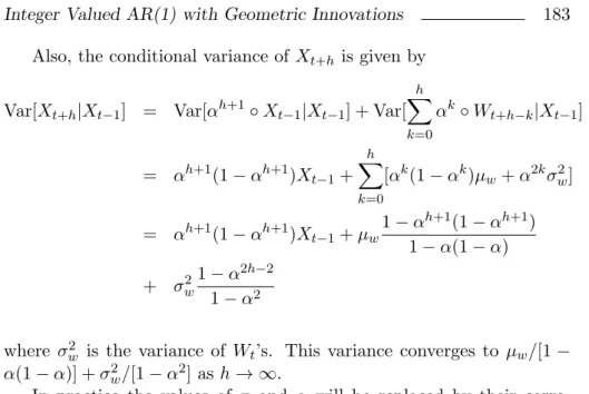
Also, the conditional variance of Xt+h is given by
Var[Xt+h|Xt−1] = Var[αh+1◦Xt−1|Xt−1] + Var[
h ∑ k=0
αk◦Wt+h−k|Xt−1]
= αh+1(1−αh+1)Xt−1+
h ∑ k=0
[αk(1−αk)µw+α2kσw2]
= αh+1(1−αh+1)Xt−1+µw
1−αh+1(1−αh+1) 1−α(1−α) + σw21−α
2h−2 1−α2 where σ2
w is the variance of Wt’s. This variance converges to µw/[1−
α(1−α)] +σ2w/[1−α2] ash→ ∞.
In practice the values of π and α will be replaced by their corre-sponding maximum likelihood estimates.
4
Simulation
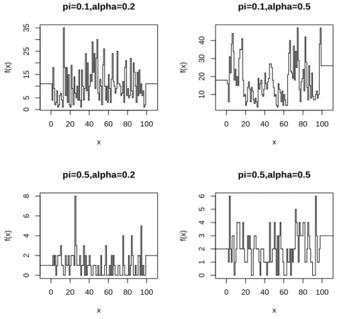
Figure 1 shows the sample paths of simulated INAR(1) processes with Ge(π) innovations for π = 0.1,0.5 andα = 0.2,0.5. As we can see from (7) and (8), for largerαand lessπ we have larger mean and variance so a tendency to yield larger values, but for smaller values ofα and larger π sample paths tend to smaller values and frequently returns to zero with less mean and variance.
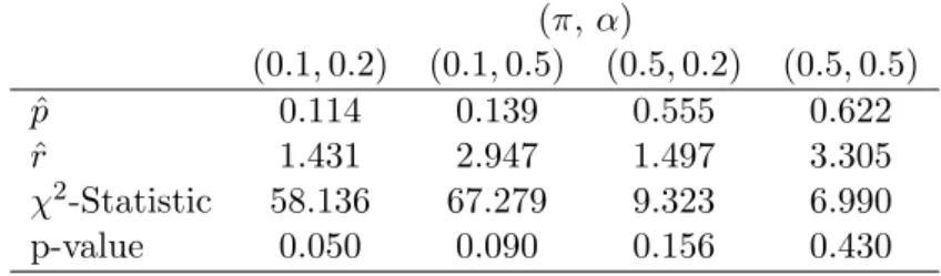
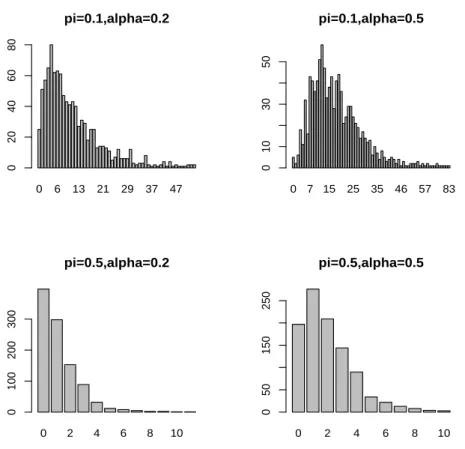
Figure 2 and the corresponding Table 1 illustrate the marginal distri-butions of the simulated series as described above. The bar plots show that for large π and smallα, the empirical marginal distribution decays geometrically, whereas for smaller π, and particularly for larger α, the marginal distribution begins to resemble a more complex mixture, as we expected by Remark 2.2 and the pmf (15). We propose negative binomial for the limiting marginal distribution of the INARG(1), be-cause negative binomial distribution, nb(r, p), can arise as a mixture of Poisson distributions with mean distributed as a Gamma(r,(1−p)/p) distribution. In this model, the mean and variance are r(1−p)/p and r(1−p)/p2, respectively, wherein p and r can be easily estimated via moment method. The goodness-of-fit tests confirm that in this case the negative binomial gives a reasonable fit to the marginal distribution.
Table 1: Goodness of fit of negative binomial model for marginal distri-bution of INARG(1)
(π, α)
(0.1, 0.2) (0.1, 0.5) (0.5, 0.2) (0.5, 0.5) ˆ
p 0.114 0.139 0.555 0.622
ˆ
r 1.431 2.947 1.497 3.305
χ2-Statistic 58.136 67.279 9.323 6.990
p-value 0.050 0.090 0.156 0.430
Table 2 contains the mean and mean squared error (MSE) of es-timates by the conditional maximum likelihood (CML) estimation and approximate full maximum likelihood (AFML) estimation methods. The estimates were computed by simulating 100 series (of length 100) from the INARG(1) processes for some chosen π and α. The AFML, which uses a (geometric) approximation to the marginal pmf (for larger π) for the first observation, performed very slightly better than the CML which ignores (conditions on) the first observation. However for smaller π, when we know that the approximation to the marginal is not as good, the AFML performs slightly worse. Given these results, there seems to be no advantage in using AFML for series of length 80 or more (typical of the real datasets we examine in the next section).
Table 2: Mean (MSE) of estimates from fitting INARG(1) by CML and AFML
( π, α) πˆ αˆ
(0.1,0.2) AFML 0.09806 (0.00050) 0.20645 (0.00136) CML 0.10297 (0.00012) 0.20378 (0.00123) (0.1,0.5) AFML 0.09782 (0.00061) 0.51485 (0.00202) CML 0.10436 (0.00016) 0.50751 (0.00072) (0.5,0.2) AFML 0.50398 (0.00183) 0.19586 (0.00689) CML 0.50348 (0.00185) 0.19603 (0.00690) (0.5,0.5) AFML 0.50718 (0.00175) 0.50712 (0.00352) CML 0.50713 (0.00176) 0.50713 (0.00352)
0 20 40 60 80 100
0
5
15
25
35
pi=0.1,alpha=0.2
x
f(x)
0 20 40 60 80 100
10
20
30
40
pi=0.1,alpha=0.5
x
f(x)
0 20 40 60 80 100
0
2
4
6
8
pi=0.5,alpha=0.2
x
f(x)
0 20 40 60 80 100
0
1
2
3
4
5
6
pi=0.5,alpha=0.5
x
f(x)
Figure 1: Sample path of INARG(1) process for π = 0.1,0.5 and α = 0.2,0.5 .
0 6 13 21 29 37 47
pi=0.1,alpha=0.2
0
20
40
60
80
0 7 15 25 35 46 57 83
pi=0.1,alpha=0.5
0
10
30
50
0 2 4 6 8 10
pi=0.5,alpha=0.2
0
100
200
300
0 2 4 6 8 10
pi=0.5,alpha=0.5
0
50
150
250
Figure 2: Bar-plots of limiting marginal distribution of INARG(1) for π= 0.1,0.5 andα= 0.2,0.5
5
Data analysis
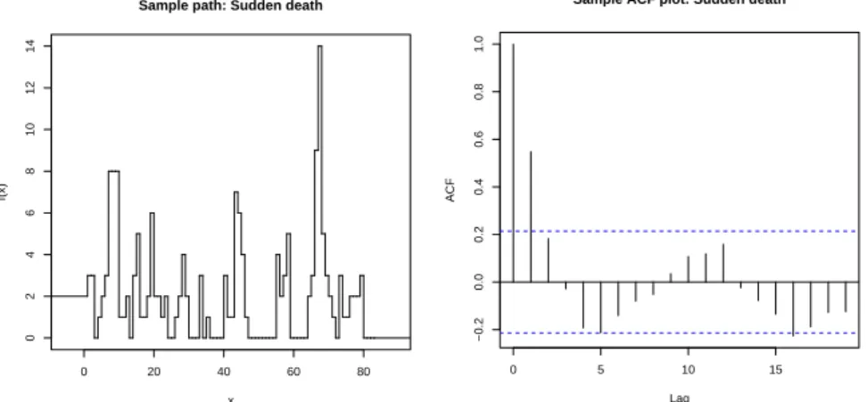
We now illustrate with some real time series data the ability of the INARG(1) to improve on the fit of the traditional INAR(1) with Pois-son innovations. Our data give numbers of submissions to animal health laboratories, monthly 2003-2009, from a region in New Zealand. The submissions can be categorized in various ways. Here we consider one series giving the total number of bovine cases, and several others catego-rized by presenting symptoms. One such is the number of submissions with sudden death, given in Table 3. The sample path and autocorrela-tion funcautocorrela-tion (ACF) of this series are shown in Figure 3. The series has a large proportion of zero values, and some long runs of zeros. The ACF
suggests first-order dependence. We would expect some positive correla-tion in such series because the underlying processes causing disease will change smoothly in time.
Table 3: Time series: Sudden death (¯x= 2.024, s2 = 6.529, f0 = 0.357, e−¯x= 0.132)
Jan Feb Mar Apr May Jun Jul Aug Sep Oct Nov Dec
2003 2 3 3 0 1 2 3 8 8 8 1 1
2004 2 0 3 5 1 1 2 6 2 2 1 2
2005 0 0 1 2 4 2 0 0 0 3 0 1
2006 0 0 0 0 3 1 1 7 6 4 1 0
2007 0 0 0 0 0 0 0 4 2 3 5 0
2008 0 0 0 0 2 3 9 14 5 3 2 1
2009 0 3 1 1 2 2 2 3 0 0 0 0
0 20 40 60 80
0
2
4
6
8
10
12
14
Sample path: Sudden death
x
f(x)
0 5 10 15
−0.2
0.0
0.2
0.4
0.6
0.8
1.0
Lag
ACF
Sample ACF plot: Sudden death
Figure 3: Sample path and ACF plot of Sudden death submissions We fitted both INAR(1) (with Poisson innovations) and INARG(1) models to Sudden death series by conditional maximum likelihood. By comparing their Akaike’s information criterion (AIC) under each model, we conclude that the INARG(1) model with Wt ∼ Ge(0.421)
innova-tions,
Xt = 0.317◦Xt−1+Wt, (17)
yields a much better fit (with AIC=305.999) than the traditional INAR(1) model (with AIC=346.4521).
By selected model (17), the predicted values of Sudden death series are
ˆ
X1 = (1−πˆ)/[ˆπ(1−αˆ)] = 2.014 and
ˆ
Xi = αXˆ i−1+ (1−ˆπ)/πˆ = 0.317Xi−1+ 1.375,
fori= 2,3, ...,84. Figure 4 shows the closeness of these predicted values to the sample paths of Sudden death series.
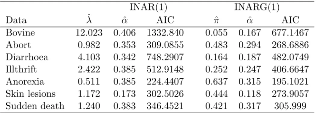
This can be repeated with the other laboratory submission series, giving the results shown in Table 4. We can see that in all cases the im-provement from the INARG(1) model is highly significant. We also com-pare the proportion of zeros f0 with e−¯x (Table 5), suggesting for each series that the proportion of zeros in the data is greater than expected from INAR(1) with Poisson innovations. It is interesting that even for the series of total bovine cases, which has few zeros, the INARG(1) fits better because the mean is large and so zeros would not be expected under the INAR(1) model.
Table 4: Fitting INAR(1) and INARG(1) models by CML estimation method
INAR(1) INARG(1)
Data λˆ αˆ AIC πˆ αˆ AIC
Bovine 12.023 0.406 1332.840 0.055 0.167 677.1467 Abort 0.982 0.353 309.0855 0.483 0.294 268.6886 Diarrhoea 4.103 0.342 748.2907 0.164 0.187 482.0749 Illthrift 2.422 0.385 512.9148 0.252 0.247 406.6647 Anorexia 0.511 0.385 224.4407 0.637 0.315 195.1021 Skin lesions 1.172 0.173 302.5026 0.444 0.118 273.9057 Sudden death 1.240 0.383 346.4521 0.421 0.317 305.999
0 20 40 60 80
0
2
4
6
8
10
12
14
Predicted values: Sudden death
x
sfun1 (x)
Figure 4: Predicted values of Sudden death series
Table 5: Observed (INAR(1)) proportion of zeros of the laboratory sub-mission series
Data f0 e−¯x
Bovine 0.071 1.21E-09
Abort 0.440 0.223
Diarrhoea 0.214 0.002 Illthrift 0.238 0.020
Anorexia 0.667 0.440
Skin lesions 0.405 0.240 Sudden death 0.357 0.132
Acknowledgements
We thank Lachlan McIntyre of the Ministry of Agriculture and Forestry, New Zealand for providing the data on animal health laboratory sub-missions. We also thank an Associate Editor for his/her careful reading of the manuscript and helpful comments.
References
Al-Osh, M. A. and Alzaid, A. A. (1987), First-order integer-valued autoregressive (INAR(1)) process. Journal of Time Series Analysis Econometrics, 8, 261-275.
Alzaid, A. A. and Al-Osh, M. A. (1988), First-order integer-valued autoregressive (INAR(1)) process: distributional and regression properties. Statistica Neerlandica,42(1), 53-61.
Du, J. G. and Li, Y. (1991), The integer-valued autoregressive (INAR(p)) model. Journal of Time Series Analysis,12, 129-142.
McKenzie, E. (1985), Some simple models for discrete variate time series. Water Resources Bulletin,21, 645-650.
McKenzie, E. (1986), Autoregressive moving-average processes with negative binomial and geometric marginal distributions, Advanced Applied Probability,18, 679-705.
Park, Y. and Oh, C. W. (1997), Some asymptotic properties in INAR(1) processes with Poisson marginals. Statistical Papers,38, 287-302. Pavlopoulos, H. and Karlis, D. (2006), On time series of overdispersed count: Modelling, inference, simulation and prediction. Technical Report, Department of Statistics Athens University of Economics and Business, 221, 1-38.
Pavlopoulos, H. and Karlis, D. (2008), INAR(1) modeling of overdis-persed count series with an enviromental application, Environ-metrics, 19, 369-393.
Silva, M. E. and Oliveira, V. L. (2004), Difference equations for the higher-order moments and cumulants of the INAR(1) model. Jour-nal of Time Series AJour-nalysis,25, 317-333.
Steutel, F. W. and van Harn, K. (1979), Discrete analogues of self-decomposability and stability. The Annals of Probability, 7(5), 893-899.
Steutel, F. W. and van Harn, K. (2004), Infinite divisibility of proba-bility of distributions on the real line, New York: Marcel Dekker.