Jonathan B. Moore. Evaluating the spectral clustering segmentation algorithm for describing diverse music collections. A Master’s Paper for the M.S. in L.S degree. May, 2016. 104 pages. Advisor: Stephanie Haas
This paper presents an evaluation of the spectral clustering segmentation algorithm used for automating the description of musical structure within a song. This study differs from the standard evaluation in that it accounts for variability in genre, class, tempo, song duration, and time signature on the results of evaluation metrics. The study uses standard metrics for segment boundary placement accuracy and labeling accuracy against these song metadata. It reveals that song duration, tempo, class, and genre have a significant effect on evaluation scores. This study demonstrates how the algorithm may be evaluated to predict its performance for a given collection where these variables are known. The possible causes and implications of these effects on evaluation scores are explored based on the construction of the spectral clustering algorithm and its potential for use in
describing diverse music collections.
Headings:
Music libraries
Sound recordings
Information storage & retrieval systems – Audiovisual materials
Library Automation
EVALUATING THE SPECTRAL CLUSTERING SEGMENTATION ALGORITHM FOR DESCRIBING DIVERSE MUSIC COLLECTIONS
by
Jonathan B. Moore
A Master’s paper submitted to the faculty of the School of Information and Library Science of the University of North Carolina at Chapel Hill
in partial fulfillment of the requirements for the degree of Master of Science in Library Science
Chapel Hill, North Carolina May 2016
Approved by
Table of Contents
I. Introduction ... 2
II. Review of the Literature ... 5
Bag-of-Features ... 8
Sequence-Based Analysis ... 12
Structural Sequence ... 13
Spectral Clustering ... 20
Evaluation ... 22
III. Methodology ... 31
Overview ... 31
Tools and resources... 33
Procedure ... 36
Research Questions ... 37
IV. Results ... 40
Summary ... 40
Genre ... 41
Class ... 42
Tempo ... 42
Song Duration ... 43
Discussion ... 44
Results tables ... 52
Results figures ... 55
V. Conclusion ... 65
References ... 66
APPENDIX 1. Song metadata by Song ID ... 69
APPENDIX 2. Evaluation results by Song ID ... 78
APPENDIX 3. Abbreviations and acronyms ... 87
APPENDIX 4. Time and Frequency Representations (TFRs) ... 89
The Spectrogram ... 89
Mel Frequency Cepstral Coefficients ... 92
The Constant-Q Transform ... 94
I.
Introduction
As new technologies have opened up new ways to study music, they likewise have
created new applications for this research. Among these is Music Information Retrieval
(MIR), an interdisciplinary field of study that examines methods of providing access to
musical data. Modern research in MIR seeks innovative ways of indexing a digital
collection of music that can be applied in search engines, recommendation services, and
scholarly databases. These strategies are built upon our ability to describe musical
similarity and which songs are similar in certain ways to other songs. There are multiple
things one can take into account for this task, including but not limited to the following
factors. 1) The bibliographic information that accompanies a piece of music: its title,
composer, lyricist, date of composition, etc. 2) The social component: what are the
listeners of this piece of music like and how can we use that to predict who else might be
interested in the piece of music? 3) The subjective qualia of the music: how might one
describe the experience of listening to this piece of music and does that make it more
suitable for certain moods or activities? 4) The aural qualities of the music itself: the
relationships between notes, harmonies, rhythms, and other qualities that are revealed in
the content of the music. The subject of this particular study is musical structure, which
fits within that fourth factor and comprises that quality of a piece of music which allows
us to identify themes and sections which repeat within the piece. The study of musical
melody, rhythm, and timbre. Structure has historically been a primary component in
determining how to classify a piece of music; terms like rondo, fugue, and sonata double
as both structural and genre descriptors in the Western Classical tradition, and even more
modern genre classifications like blues and pop often imply a defined structure. This
study of musical structure is certainly central to any debate about musical description.
Naturally, we cannot expect every digital collection of music to be structurally
analyzed by a music theorist, but there are nascent methods of automating the task. These
processes, known as structural segmentation algorithms, are able to parse a digital audio
file and discern its repeating sectional components. Usually, these algorithms are
evaluated in an adversarial way, i.e. competing algorithms are tested against one
collection and ranked according to the which algorithms maximize or minimize the
values returned by standardized evaluation metrics that measure, for instance, the
accuracy of the placement of sectional boundaries or the agreement between sections that
an algorithm determines are alike and those determined by a human expert to be alike..
This study proposes another kind of evaluation using just one subject algorithm against
the same standardized evaluation metrics. This method of evaluation is not to determine
which algorithm among many receives the highest average evaluation score, but instead
to determine what variables within a collection have a significant effect on the evaluation
scores that a single algorithm receives.. In this case, I will examine the performance of
the spectral clustering algorithm proposed by McFee & Ellis [1] against ground truth
segmentations in a collection in which broad genre classification (referred to as class),
narrow genre classification (referred to as genre), the division of beats within a bar
duration for each song are known. . It could be used to identify the weaknesses of an
algorithm or to determine particular types of collections to which an algorithm is or is not
suited. The basic research questions may then be stated as follows:
1) Do either broad class or narrow genre of a song have a significant effect on the
accuracy of the spectral clustering algorithm for the structural segmentation of
that song?
2) Is there a significant correlation between the duration, tempo, or time signature of
a song and the accuracy of the spectral clustering algorithm for the structural
II.
Review of the Literature
As a field of study, MIR rests within the larger field of Information Retrieval (IR).
Therefore, its beginnings lie in research first pioneered for text-based documents in
traditional search contexts. The earliest music search systems developed under this
standard relied on textual metadata for retrieval. Fields that you might find as part of a
traditional card catalog formed the basis for access: searching for music by a known
composer, or with a known title, or from a known album, or published in a particular
year. This model is sufficient for the kinds of basic searches done by reasonably informed
users on collections that are well described. Even modern applications largely rely on the
prototypical formula. As an example, the music used in this study was purchased from
the iTunes store using keyword searches that returned those pieces of music in which the
title, artist, or some other field matched the given keywords. From an academic context,
where searches might require more rigorous methods of retrieval, consider the description
of the catalog of Naxos Music Online1, which maintains a vast and comprehensive
controlled vocabulary across dozens of metadata fields to provide effective access to its
users. The methods of description vary in complexity and efficiency, but have in common
a dependency on a well-trained cadre of catalogers accurately describing large
collections. Not only is this a time- and resource-intensive process, it is also one with
on the largely subjective terminology of genre and style, and explicitly musical qualities
(including tempo, key, or chord progressions) require exhaustive analysis to evaluate
even in the few cases where they are unambiguous. As the number of pieces of music
continues to grow, and services seek to provide access to ever-larger numbers of them,
searching based on some measure of musical similarity using traditional means of
musical analysis by experts is just impractical.
One popular workaround is to crowd-source description tasks. Organizations like
MusicBrainz2 draw on the efforts of a community of enthusiasts where many amateur
users may each submit their own metadata as tags. In this system, the agreement of many
of these users on a set of metadata substitutes for the pronouncement of one or a few
expert catalogers. Referred to as social-tagging, this metadata arrives unrestricted and
unstructured; the process democratizes the descriptive task on the predicate that
popularity is a predictor of accuracy. Given their lack of editorial influence, these tags
can potentially cut across any and all potential categories of description. Genre, key, time
signature, lyrical subjects, the appropriate mood for listening, even the internal memes of
the tagging community may coexist as relevant labels. [2] shows us that this approach has
real advantages over bibliographic search, but disadvantages as well. The social interest
across all pieces of music is not evenly distributed, with a small minority of music
receiving the lion’s share of attention and tags, and the long tail of music that remains
being so meagerly described as to make meaningful tags hard to distinguish from
meaningless noise. In cases where one is primarily concerned with only the most
well-known music this might be sufficient, but the effectiveness of social-tagging for a piece
access, penalizing obscurity can be counterproductive. To consider all pieces of music
within a collection uniformly, researchers have considered ways to incentivize a user
base to consider tracks they might not have otherwise considered. For instance, [3]
discusses how the process of tagging might be gamified to encourage users to tag more
evenly and comprehensively. Yet attempting to control the behavior of large crowds is
never a simple or reliable process.
A similar hurdle once faced text-based IR. That field has since benefitted from
volumes of research focused on discerning the semantic qualities of documents without
relying on human description. The potential of this research for internet applications,
where personal examination of the vast quantities of documents on the web would be
inconceivable, injected a new urgency into the field in the 80s and 90s that ultimately
gave us the modern search engine and with it the ubiquity of Google (whose
searches-per-year surpassed 1 Trillion in 20113). The web-search renaissance was built on the
basic ability to parse and estimate the semantic relevance of textual documents digitally,
but such a task is not so easily replicable with musical content. Text is divisible into
letters: well-defined elements that can be represented as a standard string of binary data,
the collection of which can represent a word. Words exist as independent entities with
relationships that we can categorize in dictionaries and thesauri. Without needing to
understand the meaning of words, larger semantic concepts like topic can be
algorithmically estimated based on relatively straightforward functions like word
occurrences across an index. Music must work with a different kind of data that cannot be
understood in the same semantic way that text is. This is not to say that automated
methods to achieve similar results. [4] identifies two techniques that persist in popularity
in the MIR community. The first is based on the foundational work previously discussed
in tagging music, with the distinction that the tagging is not done socially but rather
algorithmically based on the feature analysis of the signal. The second focuses on
creating relevance judgements using patterns in the time and frequency representation
(TFR) of the music itself without the mediation of a semantically meaningful tag. [4]
labels these as the “Bag-of-Features” approach and the “Sequence-based” approach. The
following section will detail the ways digital music data is used for content description
and the strengths and weaknesses of major approaches that have informed the creation of
the structural segmentation algorithm. The final section will discuss approaches to
evaluating structural segmentation algorithms and how this study differs from those
approaches.
Bag-of-Features
The bag-of-features (BoF) approach is so called because it bears some similarity to the
words conceptualization of a document used in text-based IR. Like the
bag-of-words approach does with bag-of-words, the bag-of-features approach to content analysis
separates some kind of identifiable element from within the piece of music and considers
it as a solitary unit outside of the particular context in which it appears. Which kind of
feature being considered usually gives the particular implementation of this approach its
name; researchers call it alternatively by the names of-features, of-frames,
bag-of-audio-words, bag-of-systems, and so on to distinguish the particular qualities being
bagged in their approach [5]—[10]. Common to all approaches is a set of tags tied to a
collection commonly associated with those tags. A machine-learning process of some
variety is typically employed to improve the accuracy of the probabilistic tagging feature
[9][10]. Tags are often pre-defined according to some controlled vocabulary, although
this approach can be combined with social tagging to develop an unbound dictionary of
tags tied probabilistically with identifiable features as in [2]. Accordingly, these
automatically generated tags may theoretically take any form: genre, instrumentation,
mood, etc. and are therefore well-suited to search systems in which an end-user is
searching for music based on a keyword query-by-text. While the variety of approaches
that fall within the BoF framework are too numerous to go into in fine detail, one can
nonetheless outline the common process of generating a BoF representation as [8] did in
fig. 1.
The first few steps, from audio signal to feature extraction, are just as previously
outlined. Preprocessing refers to any step that must be taken to prepare a digital audio file
for signal analysis, including changing the file format or other such tasks. To
disambiguate, in fig. 1 the term “segmentation” refers to the process of segmenting an
audio signal into frames by a window function. Once a TFR for an audio signal is
created, the BoF approach must quantize the vectors of the TFR. In other words, they
must identify some number n of relevant values per some subdivision in the TFR and
map them to a vector of n dimensions. This vector is then predicted to belong to some
defined feature vis-à-vis a probability model in that vector space, where probability is
determined based on an initial sample set of data for which both vectors and feature tags
are known.
A common approach is to
employ a nearest-neighbor calculation
between the given vector and the
nearest known sample vector. While
difficult to visualize in vector space of
more than 3-dimensions, the idea is
that one can predict which feature is
represented by a new vector simply by
determining which feature is
represented by the nearest known
vector (by Euclidian distance). This is
the basic approach used in [8][11]. This approach has drawbacks, notably that one must
compute each new vector against all known vectors as they are generated. An alternative
proposed in [9] is to define some parametric function in the vector space for which the
output is the probability that the vector belongs to a certain feature. Using a parametric
probability function requires less computational effort, making it more suited to large
collections. These probability functions are most often defined using a Gaussian Mixture
Model (GMM), in which multiple Gaussian distributions of probability simulate a
continuous probability function[9][10][12], although alternative or modified
constructions are not uncommon[6]. The audio signal is thus reduced to a collection (or
bag if you will) of these feature vectors for which each is said to belong to a probable
feature. That feature for each vector is taken from the vocabulary of tags that is
determined by the sample data. The data can then be represented by a histogram of all
tags in the vocabulary and their cumulative probability of occurrence in the song as in fig
2.
While research continues to make progress in improving BoF approaches to
music content-analysis, [5] identifies persistent problems that limit its general application
at least to polyphonic music (music with many voices or sources of sound that do not
always produce sound in unison). One, BoF methods usually cannot improve beyond a
maximum precision (about 70%) that is not affected by extenuating factors, which [5]
calls the glass ceiling. Two, means of modeling dynamic changes in the audio signal in
BoF approaches offer no improvement over static models despite their significance in the
perception of a listener. Three, intriguingly there seems to exist a class of polyphonic
songs which are found to be consistently returned as false positives in BoF MIR tasks
regardless of the circumstances of the search; these songs are called hubs. Additionally,
[4] identifies the more general weakness that, while BoF approaches may succeed in
identifying features accurately, they ignore the context in which the features exist and the
behavioral relationships between them within the song. For instance, in principle one
could use tags to identify the number major and minor chords are present in a song, but
not the movement between major in minor chords across a song. Likewise, one could use
tags to identify a saxophone in a song, but not where in the song it plays a solo. These
descriptions and those like them, while they may not be useful for the lay searcher, are
imperative in a musician’s conceptualization of a piece of music. For these tasks, we
must look beyond the paradigm of traditional metadata description using text established
by the practices of card catalogues. One must be able to describe temporal and structural
Sequence-Based Analysis
When describing temporal and structural patterns, one is not looking merely for the
presence of some values, but the relationship of those values to the values around it. This
requires knowledge of the order of values; in other words, we must examine not just the
values but the sequence of values. For example, consider these three sequences of
integers: “1,2,3,4,5”, “1,2,3,5,4”, and “2,5,3,4,1”. Approaching this with a BoF
framework would allow us to identify the equal occurrence of the same values in each
sequence, and therefore equal similarity among all sequences. However, given
“1,2,3,4,5” as a query, one nonetheless would likely want to identify ”1,2,3,5,4” as being
more similar or relevant than “2,5,3,4,1”. The body of sequence-based approaches to
retrieval depends therefore on the ability to quantify the degree of similarity between two
comparable sequences of values [4]. This is called sequence alignment. In general,
sequence alignment seeks to generate an alignment score between sequences, such that
the highest scoring sequence can be said to be the most similar to the query sequence.
The specific process, however, depends on the class of values that make up the sequence
being examined. Certain important features in music can be understood only as a
sequence. For instance, a melody is a sequence of pitches; a chord progression is a
sequence of harmonies; even a piece of music itself can be considered a sequence of
repeating sections. The accuracy of sequence alignment as a process then depends on
how accurately one can identify the values that make up these sequences: pitches,
harmonies, sections. Significant progress has been made in the field of melodic
transcription of polyphonic audio, but the task has not yet advanced to the degree that it
[4]. The reader is referred to [13] for a review of pitch tracking systems in melodic
transcription and to [14] for a comprehensive overview of digital melodic transcription
research. Although melodic transcription is not yet applicable in writ large, significant
advancements have been made in sequence-based analysis based on the final two
examples, chord sequence and structural sequence. This review will only discuss the
research into the latter, although a discussion of chord sequence estimation and its
foundational work in identifying musical “states” can be found in appendix 5. The
following will refer to TFRs known as the Mel Frequency Cepstral Coefficients (MFCC)
and the Constant-Q Transform (CQT) in some detail. See appendix 4 for a full definition
and discussion of these types of TFRs that are used in musical content analysis and
specifically in the spectral clustering algorithm.
Structural Sequence
The analysis of structural sequence is a way to identify and order the states that are
emergent within the signal, the musical form. While computationally difficult, this is a
process that even lay listeners perform almost subliminally when listening to a piece of
music. It is the process by which a listener can infer, for instance, that the chorus of a
song has moved to the verse. These states within the music, which may colloquially be
referred to as a section or part, are conditional on their relationship to other states; that is
to say, you cannot logically have a song that is all chorus and you cannot have a bridge
without the two sections that it bridges. It is the repetition, or lack thereof, and order of
these emergent states which allow us to classify them. Despite how naturally a human
listener may be able to identify these sections, the computational equivalent referred to as
segmentation has proven to be a challenge. [15] proposes that sections within a piece of
Homogeneity refers to those consistent elements within a section that allow us to say that
it is one single unit; novelty is the contrast in elements that marks a break in homogeneity
and thus a new section; and repetition is that feature that marks the recurrence of a
previously-occurring section. These relationships must be determined by some features
that can be represented in a TFR, although which features most clearly establish the
relationships may vary. Accordingly, approaches to the structural sequence problem use a
variety of TFRs with a variety of specialized uses as a starting point, and there is as yet
no one TFR that is clearly best-suited. [16] established in 2001 that the MFCC generally
outperformed other TFRs if the focus of segmentation rested on timbre; however, new
research and new applications since then have broadened the horizons. While the MFCC
continues to be used in many studies, it appears in the corpus alongside, and indeed often
in conjunction with, chroma features and to a lesser extent the CQT as well as many less
common TFRs [15].
Regardless of the TFR used, a specialized representation is used for segmentation
that has not yet been discussed. Rather than visualizing the frequency against time in a
signal, segmentation requires some method of measuring homogeneity, novelty, and
contrast. For this, we do not need to know the specific values of frequency features, but
rather some measurement of the relative similarity and distance of these features to one
another. [17] proposed a metric known as the self-similarity matrix (SSM) that allows for
this. Given two vectors, which in this case represent the values of two frames of some
TFR, [17] asserts that the scalar product of the two vectors may be used as a similarity
metric. [15] notes that Euclidean or cosine distances between the vectors are also
frame, one can construct a square matrix
with the values representing the distance
between every combination of vectors. If
represented as a heat map, one should find
that the values are lowest along a center
diagonal of the matrix, representing the
distance between each frame and itself.
Diagonals parallel to the center diagonal
represent low distances between one
succession of frames and a separate
succession of frames. This can be used to identify repetition. Square regions of lower
values along the central diagonal represent a localized section of frames that have low
distances among themselves. This can be used to identify homogeneity. Regions of high
distance values near the central diagonal represent frames that are near to each other in
time but have a large distance metric. This can be used to identify novelty. These features
can be seen in fig 3.
With a given self-similarity matrix, it follows that the next undertaking is to
describe some computational method of identifying these relevant repetition,
homogeneity, and novelty features. Different algorithmic approaches often prioritize one
of these three qualities [15]. Additionally, within these three categories of approach, there
are two goals to which an algorithm might aspire. The first is boundary detection, in
which the aim is to identify the points in time in the signal that delineate where sections
begin and end. The second is labeling, which focuses on grouping sections by the
likelihood that they are alike. Segmentation algorithms typically accomplish either
boundary identification only or both boundary and label identification.
In early boundary identification experiments, [18] attempted boundary
identification without a full SSM representation, simply by calculating the Mahalonobis
distance between vectors of successive frames in multiple TFRs; however, this method
suffers in that the scope of frame-to-frame novelty does not take into account the context
of the frames. That is to say, sometimes, a boundary cannot always be identified as
change in a single instant. [19] builds on the original SSM research by introducing a
boundary algorithm that prioritizes novelty of a region. In this method a
checkerboard-like kernel with a Gaussian radial function (a visualization can be seen in fig. 4) with a
given size, or duration, iterates across the central diagonal of the SSM. The correlation
between the values in the kernel and the values in the SMM are measured and plotted
against the duration of the song producing a novelty curve. Where the regions of high and
low similarity conform closest to the checkerboard shape of the kernel, the correlation
and thus novelty is high. This shows the location of box corners of high and low distance,
where regions of high similarity are separated by regions of high distance. High values in
the novelty curve suggest that a location is a
logical boundary point between sectional
regions.
[20] proposed an improvement to the
standard novelty curve for boundary
identification that includes both local novelty
and a model of global novelty. In the proposed
method, each vector of a given TFR is concatenated with the values of preceding vectors
according to some duration parameter. This produces a series of high-dimensional nested
vectors that retain a kind of “memory” of the recent past. A novelty curve against a
time-lag transformation of these vectors yields boundaries that more accurately captures
transitions between inter-homogenous sections rather than simply the highest points of
local novelty. In [21], the authors build upon the work of [20]. They do away with the
novelty curve altogether and instead reduce the memory-informed self-similarity matrix
to a fixed-dimensional (i.e. duration-independent) matrix of latent repetition factors that
capture transitions between repetitive and non-repetitive sections. [22] formulates an
alternative method of regional boundary identification from homogeneity rather than
novelty. A cost function is utilized that computes the sum of the average self-similarity
between successive frames of a signal. The task of the function is to group as many
frames together as possible given a cost parameter that penalizes grouping frames with
low self-similarity. By increasing the value of the cost parameter, the number of possible
segments decreases. This allows control over the function in its implementation that
prevents spurious or too-frequent boundary identification.
[18] and [19] both note that boundary identification alone can be useful for
example by facilitating audio browsing (where the listener may want to jump between
meaningful sections rather than attempting to locate them via traditional fast-forwarding
and rewinding). However, simply identifying boundaries does not provide meaningful
descriptions of the relationships between sections. Repetition-based methods have
approached labeling visually, as a task of identifying the diagonal stripes parallel to the
false stripe identification, and they rely on the assumption that all repetitions occur in the
same tempo (changes in tempo result in a distortion in the shape of a stripe, angling it
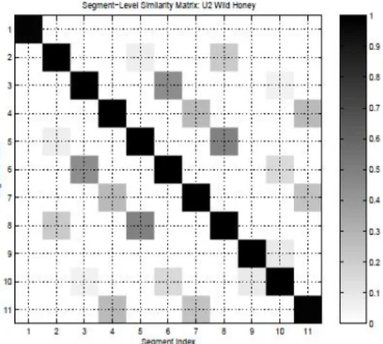
towards or away from the diagonal) [15]. In the first approach to some kind of label
identification, [23] sought to combine the novelty-seeking kernel boundary algorithm of
[19] with a homogeny-seeking clustering algorithm that compares the Singular Value
Decomposition (SVD) of the regions between novelty-identified boundaries. The SVD is
computed as a function of the relationship between the empirical mean and covariance of
the spectral values in the TFR for each segment. This SVD takes a value between 0 and
1. These SVD values are then used to create a segment-indexed similarity matrix (seen in
fig. 5). High SVD values indicate that two segments should be grouped under the same
label. This is a highly versatile method that [23] notes could be used to identify structural
similarity even in image or video data; however, the process is computationally intensive.
Furthermore the similarity between segments determined by SVD is unable to account for
changes in key that do not affect the underlying structure. In other words, where a human
might recognize a section in one key with a certain melody, and a section in another key
with the same melody as belonging to the same
section, the SVD cannot. [24] proposes a novel
alternative to clustering by SVD using a
calculation of the 2D-Fourier Magnitude
Coefficients (2D-FMC) of each segment. This
has the dual advantage over the SVD in that it
is computationally simpler and key-invariant.
In this implementation, the 2D-FMC used can
be described as a segment-length-normalized matrix of values that measures in two
dimensions the frequency-amplitude of some segment of chromagram the way that a DFT
measures in one dimension the frequency-amplitude of a signal. The distance relationship
between the 2D-FMCs for each segment can be plotted against each other in a similar
segment-indexed similarity matrix.
These methods are largely successful in applying labels but they are nonetheless
dependent on an independent boundary identification algorithm. [25] the “constrained
clustering” algorithm holds that the identification of recurring sections can more
efficiently be done using an E-M trained HMM to identify section states similar to the
models used in chord identification (see appendix 5). The process by which this occurs
uses what is essentially a continuous, adapted BoF approach that reduces some frame
within a TFR to a histogram of feature probabilities. These probabilities are related to
some probability model of states for which the states involved correspond to expected
structural sections types in the vein of “chorus,” “verse,” “intro,” etc. Unlike [23], this
method has the ability to describe sections meaningfully even if there is no repetition of
them within a song. Additionally, the process can optionally be refined with the addition
of an independent novelty-seeking boundary identification mechanism which can be used
to introduce “cannot-link constraints” that define frames which should not be linked with
the same label. Unfortunately, the general applicability of the method is limited given
that it requires foreknowledge of the type of music to which it is being applied in order to
Spectral Clustering
The spectral clustering algorithm proposed in [1] offers a dual-purpose alternative that is
more generally applicable: a method of both a boundary and labeling identification based
on the graphical interpretation of a transformation of the SSM proposed based on
concepts in spectral graph theory. The algorithm does not generate a novelty curve across
the central diagonal and relate the sections that fall within these boundaries. Rather, it
seeks to explicitly identify nested or hierarchical sections by analyzing the SSM at
narrowing levels of granularity and relates the identified sections via a combination of
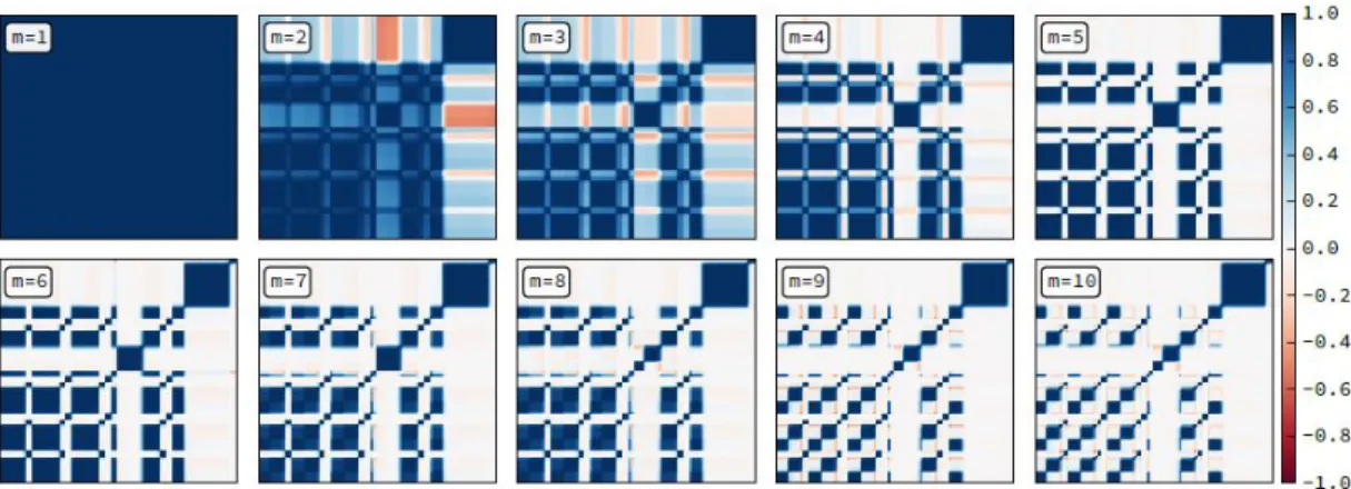
local timbre features and long-term harmonic features. One way to express the practical
implications of this narrowing granularity is that it seeks at each step to separate a given
signal that is assumed to be completely homogeneous into two identifiably distinct
divisions. The first step divides the most distinct, like sections from the rest of the song;
the second divides the most distinct, like sections from what remains; the third from what
remains of that; and so on and so on up to some parameter of steps set by the algorithm.
This process is visualized in fig. 6, where the parameter, m, is set at 10. The process by
which it arrives at this solution is explained subsequently.
The procedure can be divided into 2 parts: the construction of a graph suitable for
analysis and the analysis of the graph. First, a CQT of a signal is generated. This TFR is
chosen based on its ability to capture long-term harmonic patterns. The CQT is
mean-aggregated to the beat level; that is to say, the frames of the CQT that fall within a single
beat are collected together as a single frame for which the spectral vector values are a
mean of the vector values of the frames that fall within that beat. A memory-informed
CQT is constructed according to the precepts of [20] from the beat-synchronous frames
where each frame is concatenated with the frame that immediately precedes it. A
specialized SSM is constructed from the resultant modified CQT according to a
nearest-neighbor calculation. In this form, the values between each pair of frames is not a linear
distance metric. Instead it is binary: 1 for two frames that are determined to be nearest
neighbors in the vector space and 0 for all other frames. This produces an SSM that
enforces representation of only the strictest similarity; however, the representation
produces a field of points rather than smooth lines. The representation must then be
filtered to more clearly show patterns of similarity. This is done with the aid of an MFCC
representation of the signal, chosen because it more accurately represents local patterns in
timbre. A beat-synchronous MFCC is constructed from the first 13 mel frequency
cepstral coefficients. The relationship between the CQT and the MFCC representation are
used to generate a filtered representation of the SSM intended to capture the affinity
between local and global sequences of similarity called the affinity matrix. The full
calculation of this affinity matrix is outlined in the proposal of the method in [1].
Once this affinity matrix is generated, the concept of the Laplacian from spectral
the graph in that it measures the diffusion of points in the affinity matrix. Clustering
occurs based on this diffusion of points, where regions of less-diffuse points can be said
to constitute a region of homogeneity in the graph. This is done progressively according
to the m smallest eigenvectors of the Laplacian. These eigenvectors measure the rates of
diffusion such that they progressively increase in complexity. The first eigenvector
encodes membership in the complete set. The second encodes the clearest differential in
diffusion. The third encodes the clearest differential in diffusion of the result, and so on
up to the eigenvector m which is a parameter. The higher the value of m, the more the
diffusions will be differentiated and thus the more segments will be identified; however,
higher m attempts to measure granularity in the affinity matrix so fine that it becomes
sensitive to errors in the representation. There is also the simpler problem of
over-segmentation. As [1] notes, the challenge of the spectral clustering algorithm is in
defining the parameter m without “a priori knowledge of the evaluation criteria,” or in
other words, without some information about the required level of granularity. One
possible application of this study is to determine the effect of certain known qualities of
diversity in a music collection that may be known a priori, whether by expert knowledge
or estimation by some independent automated system, on the performance of the spectral
clustering algorithm. This will reveal which of these qualities are correlated with worse
segmentation accuracy, whether by over- or under- segmentation, and thus suggest which
qualities may require adjustment of the algorithm.
Evaluation
Before moving on to the evaluation of spectral clustering performed in this study, it will
task and exactly what they are supposed to evaluate. Segmentation evaluation falls under
the purview of the Music Retrieval Evaluation eXchange (MIREX), a community of MIR
researchers that organize a yearly presentation of evaluation results of state-of-the-art
MIR algorithms. MIREX, which began officially in 2005, has since been the primary
conduit through which MIR evaluations are conducted [26]. In order to provide robust
evaluations that can be said to be generalizable across multiple tools and algorithms,
MIREX seeks to standardize 3 components of the evaluation process: 1, standardized
tasks or queries to be made of collections; 2, standardized evaluation metrics that
measure success at these tasks; and 3, test collections of significant size to allow for these
tasks and evaluations to be run [27].
The simplest evaluations concern only the boundary identification task and are
focused on measuring the difference between the boundaries estimated by an algorithm
and known boundaries. There are two accepted ways of doing this which may be used
together. The first is hit rate, which considers the accuracy of estimated boundaries by
detecting whether or not they fall within some window of time surrounding a known
boundary. Common windows are 0.5 seconds for strict accuracy, explained in [28], and 3
seconds for more lenient accuracy, explained in [25]. There are 3 values associated with
hit rate corresponding to precision, recall, and the F-measure of the two. Precision
measures the percentage of estimated boundaries that fall within a known boundary’s
window; recall measures the percentage of known boundary windows that include an
estimated boundary; and the F-measure the harmonic average of the two rates. The
second boundary evaluation is known as median deviation. [28] defines this metric as
boundary. The median is determined based on the total collection of deviations between
near boundaries. There are two values associated with median deviation: that between
known boundaries and their nearest estimated boundaries and that between estimated
boundaries and their nearest known boundaries. These are respectively referred to as the
Median Deviation E to R and Median Deviation R to E. Both the hit rate and the median
deviation may be trimmed. To trim the metric means to ignore the values generated by
the first and last boundaries. This can be useful when one does not particularly care about
an algorithm accurately labeling the point at which silence ends and the music begins
(and vice versa). When these values are less than a second from the beginning and end of
the track, that accuracy is not particularly informative for meaningful segmentation.
There are also two metrics associated with labeling identification accuracy. The
first is known as pair-wise frame clustering, defined in [25]. This value compares labeled
frames in an estimation against known labels. All frame pairs are considered against each
other. The pairs that are assigned to the same label in the estimation form the set PE, and
the pairs that are assigned the same ground-truth labels form the set PA. There are three
values that make up this metric corresponding again to precision, recall, and F-measure.
These can be calculated according to these equations (ex. 12[25]) where PWFP measures
possible under-segmentation and PWFR measures possible over-segmentation. Labelling
success can also be evaluated with the metric known as normalized conditional entropies,
described by [29]. This is a rather more complex metric that measures the amount of
missing and spurious information in a labeling estimation. The conditional entropy
measures the number of disagreements between estimated frame labels and known frame
estimations that each have full disagreement with their known labels, the song with the
most segments receives a worse conditional entropy score simply because it has more to
disagree about. The normalized conditional entropy is, aptly, a normalization of this
count that makes it segment-count-agnostic. The metric is calculated as a rate, that is to
say as a value between 0 and 1, and flipped so that better performance returns a higher
rate. There are also 3 values associated with the normalized conditional entropy
precision, recall, and F-measure, defined as (ex. 2[29]) where SO measures
over-segmentation SU measures under-over-segmentation. H(E|A) refers to the conditional entropy
of estimation to ground-truth (spurious information), H(A|E) refers to the same between
ground-truth and estimation (missing information), and Ne and Na define the size of the
estimation and ground truth respectively. The full process of arriving at these entropy
scores is outlined in [29].
PWFP = |PE|P∩PA|
A| , PWFR=
|PE∩PA|
|PE| , PWFF=
2PWFPPWFR
PWFP+ PWFR
SO = 1−logH(E|A)
2Ne, Su = 1−
H(A|E) log2Na
Structural segmentation is just one MIR task among many that are evaluated
yearly at the MIREX, and in fact it is one of the newer tasks, added first in 20094.
Nonetheless, a number of collections have since been generated that allow for
segmentation evaluations. The most recent MIREX event included 4 datasets of songs
used for segmentation evaluation5: the original dataset collected for MIREX 2009, two
Ex. 1
datasets collected for MIREX 2010, and a fourth dataset put together by the Structural
Analysis of Large Amounts of Music Information (SALAMI) research team. The
primary function of these datasets is to link commercially or freely available songs with
what is known as ground-truth boundaries and labels (boundaries and labels determined
by an expert listener) referred to as annotations. The annotations take three forms, the
simplest two of which are boundary information alone and boundary information
between simple, non-overlapping sections each with a single label like “intro,” “outro,”
“chorus,” etc.[30]. The former method of annotation is adopted by one of the MIREX ’10
datasets6 , the latter is used by the remaining MIREX ’10 dataset7 and the MIREX ’09
dataset.8 The SALAMI dataset differs from these in that it uses a unique annotation
method that follows that proposed in [31] that allows for hierarchical sections (large-scale
and small-scale) and accounts for possible similarities between different sections. For
instance, while a “solo” and an “outro” may constitute separate musical sections, it is
possible for them to share musical qualities that are similar. The method used in the
SALAMI dataset allows for a broad characterization of sections, which could capture the
musical functions of solo/outro, as well as narrower sections within these that can
illustrate the musical similarities between them [30]. The SALAMI procedure modifies
the original procedure of [31] by more strictly defining the hierarchical segmentations
along three tracks: the musical function track (“outro,” “chorus”), the musical similarity
track, and a third track which defines the lead instrument at a given point [30]. In all four
datasets, annotations are generated manually by musically-trained experts.
As mentioned, the primary function of these datasets it to link these annotations to
are built from previously existing collections of music, which carries a number of
advantages. These collections are often used for multiple MIR tasks, and so they often
include a wide variety of potentially useful data. Collections may also be assembled with
specific conditions in mind like genre breadth or specificity, or ease of access. For
example, the MIREX ’10 datasets are constructed using songs from the Real World
Computing (RWC) database, first proposed in [32] for the purpose of facilitating MIR
evaluation across a variety of genres with publically accessible music. It includes songs
from three broad genres (Classical, Jazz, and Popular) as well as a fourth component of
entirely royalty-free music, all of which were performed and recorded for the purpose of
inclusion in the RWC database 32 [32]. Songs are provided with corresponding MIDI
files and full text of any lyrics used [32]. This source database prioritizes the accessibility
of the included music and provides useful metadata, but because the included songs exist
only for use in the database and are performed by a limited set of performers, it can only
approximate the kind of variety in production and performance that a real-world
collection of music might represent. The SALAMI dataset draws from multiple
databases, including the RWC database, with a priority “to provide structural analysis for
as wide a variety of music as possible, to match the diversity of music to be analyzed by
the algorithms.”[30]. The largest component database, and the one used in the following
study, is Codaich, chosen by SALAMI for its detailed curation of metadata [30]. Songs
described in the Codaich database represent pre-existing commercial pieces contributed
from three sources: the Marvin Duchow Music Library, the in-house database used by
Douglas Eck of the Université de Montréal, and the personal music collections of the
subgenre tags, was first drawn from the Gracenote CD database9 and then edited for
clarity and consistency by the compilers of the database at McGill University [33]. The
combination of robust metadata and variety of content makes the Codaich portion of the
SALAMI dataset idea for testing the correlations between these metadata and the
accuracy of a segmentation algorithm, although this is not the traditional way the
segmentation is evaluated through MIREX.
Because databases like Codaich, which contain robust metadata on a variety of
real-world songs, necessarily use commercially available songs in their collection, the
database cannot be shared freely among researchers due to intellectual property concerns.
As [27] says, “The constant stream of news stories about the Recording Industry
Association of America (RIAA) bringing lawsuits against those accused of sharing music
on peer-to-peer networks has had a profoundly chilling effect on MIR research and data
sharing.” Instead of having the songs in these databases be shared, MIREX has adopted
an evaluation model wherein the datasets are held by one entity, MIREX itself, and
multiple researchers each submit their algorithm to MIREX to be evaluated. This
simplifies the matters of copyright by eliminating the need to share commercial music,
but results in a particular model of evaluation. Namely, with multiple algorithms being
evaluated against common collections simultaneously, the evaluations take on an
adversarial nature. Multiple algorithms are run against the same collections and the
results and results indicate their relative performance compared to each other.10 This is
helpful in determining the state of the art among participants, but time and resource
constraints prevent MIREX from examining results in finer detail [26]. Although datasets
flat; that is to say, the report evaluation results for each algorithm for each track but do
not analyze possible variations in that data using the given metadata that accompanies the
dataset. The following study will present one method of taking the evaluation metrics
used in MIREX segmentation task evaluations and examining them in finer detail using
the detailed metadata provided in the SALAMI dataset. By including metadata such as
genre, class, tempo, duration, and time signature in the analysis of the evaluation, one is
able to determine the specific relationship between these variables and the accuracy of
the algorithm. For instance, one would be able to say not just that the algorithm is
generally expected to accurately describe song structure, but to say that the algorithm is
expected to describe song structure in one genre more accurately than another, or that the
algorithm is expected to increase the accuracy of its description for songs in faster
tempos. This is done by taking the evaluation scores across a full collection, similar to the
results offered currently by MIREX, and analyzing the means and variances in these
scores according to the given metadata. This study will compare the means and variances
in evaluation scores between each genre and class and the evaluation scores and
determine whether there are significant differences. Additionally, it will find whether
significant correlations exist between tempo, duration, and time signature and the
evaluation scores and determine the strength of those correlations. We will then use the
information described previously about the spectral clustering algorithm to offer possible
explanations for these differences and describe how they might affect the practical usage
Notes
1 naxosmusiclibrary.com 2 musicbrainz.org
3 According to http://www.internetlivestats.com/google-search-statistics/#trend. Just imagine if
similar research could do something similar for music. Even something orders of magnitude less influential would be an unimaginable change in how we consume music.
4 http://www.music-ir.org/mirex/wiki/2009:Structural_Segmentation 5 http://www.music-ir.org/mirex/wiki/2015:MIREX2015_Results
6 http://nema.lis.illinois.edu/nema_out/mirex2015/results/struct/mrx10_1/ 7 http://nema.lis.illinois.edu/nema_out/mirex2015/results/struct/mrx10_2/ 8 http://nema.lis.illinois.edu/nema_out/mirex2015/results/struct/mrx09/ 9 http://www.gracenote.com/
10 A good example of MIREX results can be found at
http://nema.lis.illinois.edu/nema_out/mirex2015/results/struct/salami/summary.html
III.
Methodology
Overview
The broadly stated objective of this study is to determine how certain variables within a
diverse collection of songs may affect the accuracy of the spectral clustering algorithm in
segmentation tasks for that collection. In a general context, diversity in a collection of
music can mean that the collection contains a breadth of songs from multiple genres, of
varying durations, a wide range of years of release, multiple unique instrumentations,
many keys, tempos, styles of (or absence of) vocalists, etc. Any sufficiently defined
variable could theoretically be measured against the algorithm’s performance, but given
the strengths of the sources of data for this study described below, the specific variables
examined here will be class (broad genre category), genre (narrower genre category),
song duration, tempo and time signature. The accuracy of the spectral clustering
algorithm for segmentation tasks will be evaluated according to the metrics of median
deviation (trimmed) of the boundaries, hit rate (trimmed) of the boundaries with a 3
second window, pair-wise frame clustering, and normalized conditional entropy. These
metrics will be analyzed in terms of the variables to show the extent to which those
variables have an effect on the evaluation results. This information can be used in a
number of ways. From the perspective of someone considering implementing the spectral
clustering algorithm in describing the structure of songs in a particular collection, the
collection’s known characteristics. For instance, someone with a collection that focuses
on a single genre or genres within a single class would be able to predict the likely
performance of the algorithm specifically in relation to that genre or class. On the other
hand, someone with a collection that holds songs of varying durations could identify
more easily which songs could be described effectively by the algorithm and which might
require manual description. Being able to view multiple analyses like the one presented
here that cover different description algorithms would allow those charged with picking
among them to make a more informed decision based on their collection. Finally, in the
case of the spectral clustering algorithm that operates with adjustable parameters, an
analysis like the following can suggest possible conditions that warrant adjusting those
parameters for more accurate segmentation estimations.
In the design of the experiment there are 4 primary components:
• First, a collection of song files is needed for which the structure of the collected songs
in known. The collection must be large enough to represent a breadth of values
among the variables to be examined in the collection. Furthermore, the structure of
the collected songs must be determined with a reasonable level of expertise,
preferably by hand by a subject matter expert, independent of the estimations
provided by the structural segmentation algorithm.
• Second, a script must be utilized that is capable of creating these structure estimations
for the given collection of digital audio files using the spectral clustering
segmentation algorithm designed by McFee & Ellis [1]. The estimations created by
• Third, another script must be utilized that is capable of referencing the estimations of
the segmentation algorithm against the independent, ground-truth song structure for
each audio file. The output of this script should be a set of numerical values
corresponding to standardized evaluation metrics for structural segmentation tasks.
• Fourth, a statistical analysis will be performed on the data determining the extent to
which the known variables in the given collection affect the values of the resultant
evaluation metrics. Results will demonstrate which qualities are correlated with less
effective (lower evaluation scores) or more effective (higher evaluation scores)
performance of the segmentation algorithm.
Tools and resources
In order to realize this task, I am entirely reliant on the generous contributions of MIR
researchers who have in recent years made vast quantities of both their own data and
open-source software tools available online. Here I will provide a brief description of the
various tools used and their value to the outline above.
The particular software tools for segmentation analysis and evaluation are taken
from the Music Structure Analysis Framework (MSAF)[34], an open-source framework
written in the Python programming language by Oriol Nieto and Juan Pablo Bello and
first presented at the ISMIR 2015 conference. This software package was selected for its
versatility and the extent of evaluation options included. MSAF defines functions in
Python for five boundary algorithms and three labeling algorithms, including McFee and
Ellis’ spectral clustering algorithm. MSAF is dependent on librosa [35] for audio feature
analysis and mir_eval [36] to compute evaluations. Statistical analysis of the evaluation
Structural annotations are sourced from the SALAMI annotation data, a project of
the Digital Distributed Music Archives and Libraries lab (DDMAL) at McGill University
in Montreal [30]. This dataset provides metadata and ground-truth structural annotations
for more than 1400 songs from a wide variety of sources. The specific metadata provided
varies based on the source database of the music. While SALAMI has annotations for
songs from the Real World Computing (RWC) Music database, the Isophonics music
database, the Internet Archive music database, and the Codaich database, only music
from the Codaich database was selected for this study due to its more robust genre
classifications.11 Further metadata is provided by SALAMI in partnership with the Echo
Nest12 including duration and estimations of tempo and time signature subdivision.
Given that the songs in the Codaich database are all held under standard
commercial copyright, the individual audio files had to be purchased through
conventional means. Because SALAMI provides bibliographic data about the songs for
which it created annotations in the XML format used by the iTunes library, the iTunes
online store was selected as the means of purchase. Within the Codaich subsection of the
SALAMI annotations, there are four broad genre classifications represented – popular,
jazz, classical, and world – with 52 subgenres between them at a total of 835 pieces of
music. While it would have been ideal to have all four genre classifications represented in
this study, the collection was limited only to songs classified as popular or jazz. There
were two reasons for this choice. First was a limitation of naming conventions in classical
music – the construction of the iTunes library file provided limited metadata that was
insufficient to ensure that any particular classical track that was purchased was the
classical tradition in which many different pieces by different composers may share the
same title (e.g. “Sonatina”), and also the lack of rigorous naming conventions by
commercial music services in which a piece may be known by multiple titles or the
“artist” for a piece of classical music may be listed as alternately the composer, the
performance ensemble, or the individual performers involved.13 Second was a limitation
of the Codaich database in regards to iTunes – many pieces of music classified as world
music by Codaich appear on compilation CDs donated from researchers’ personal
collections that may once have been available in a physical format, but are not available
for purchase digitally through iTunes.14
Reducing the proposed collection to the two remaining classifications, popular
and jazz, left the total number of songs available at 415 and the number of remaining
subgenres at 33. Furthermore, the total size of the collection for this study was limited by
funding. Funds for the purchase of music was provided by SILS up to the total of $200
through a Carnegie grant program. At the iTunes-standard cost of $0.99 to $1.29 per
track, the size of the proposed collection was roughly estimated at about 165 pieces of
music. This number allowed for an even representation of each remaining subgenre at 5
songs each. After these limiting factors, the remaining songs in the proposed collection
were cross-referenced against the iTunes store to determine what was available for
purchase. Tracks that seemed to be available but could not be confirmed as a direct match
with the given metadata were passed over. Other tracks which could only be purchased as
part of a full album (increasing their cost) were only purchased if they added to the
representation of under-represented variables whether in genre or time signature. After
represented usually by 4 to 5 tracks. A full table of the songs used, including their title,
artist, and the variables used in the subsequent study, can be found in appendix 1.
Procedure
These tracks were migrated to the Linux OS environment (Ubuntu 15.10) in
which MSAF was set up to operate. Because iTunes stores purchased music in the M4A
file format while MSAF requires either MP3, WAV, or AIFF, a small script using the
FFMPEG command-line tool was written to convert all files in the collection to MP3 at a
bit-rate of 192K. Due to the requirements of MSAF, each track was named according to
its SALAMI track identification number. A second script was written in Python 2.7 to
estimate structural segmentation for each track in the collection; this script is essentially
only a wrapper for the spectral clustering algorithmic function defined in MSAF.
Likewise, this script evaluates the results of these estimations against the ground-truth
annotations and stores the scores for each evaluation metric previously outlined for each
song in a CSV file that was imported as a data table into JMP. Metadata elements sourced
from SALAMI and the Echo Nest representing the independent variables that can be
found in appendix 1 were appended to this data.
For all results, a significant effect is assumed at a confidence of 95% or p< 0.05.
Results against the nominal data of genre, class, and time signature are analyzed
according to a one-way analysis of variance. The evaluation score results are assumed to
fall along a normal distribution within each category for each variable. Between the two
categories of class, jazz and popular, a two-tailed t-test is performed against the null
hypothesis that both classes yield the same response in each evaluation metric to
test is able to show that variance in results is unlikely to be random, but it cannot
demonstrate that the independent variable of class is necessarily causing the variation.
Between the multiple categories of genre, an F-test is employed to test the null
hypothesis that there is no significant variance in the evaluation metric scores across
genres, and a t-test between each pair of genres is used to determine possible significant
differences within the collection. The F-test is likewise able to show the likelihood that
variance among the entire collection due to genre is non-random; however, the F-test
does not make any claim about specific genres within the collection in comparison to
others. For this, the t-test among paired genres is used to demonstrate possible significant
differences between them; however, these tests work with much smaller sets of data (two
genres together are often comprised of only 7 to 10 songs). This limits their ability to
comment generally on how accuracy may be correlated with specific genres, but still
gives an idea of what variances might be affecting the results of the F-test. Results
against the continuous data of song duration and tempo are analyzed according to their
Pearson product-moment correlation coefficient with evaluation results. This measures
the strength of the linear correlation between each pair of variables; however, it can be
said that even a weak correlation between two variables may still be statistically
significant. Again, a standard t-test is used to determine the significance of the Pearson
correlation. Like with the previous tests, these results are not able to determine a causal
relationship between variables. They can only show that there is a significant correlation
between the data.
Research Questions
3) Do either the narrow genre or broad class of a song have a significant effect
on the accuracy of the spectral clustering algorithm for the structural
segmentation of that song?
a. Among all genres, is there a significant difference in the measurement
of boundary hit rate, median deviation of the boundaries, pair-wise
frame clustering, and normalized conditional entropy as determined
by an F-test? And if so, are there significant differences between
genres determined by a two-tailed t-test?
b. Between the two classes, is there a significant difference in the
measurement of boundary hit rate, median deviation of the
boundaries, pair-wise frame clustering, and normalized conditional
entropy as determined by a two-tailed t-test?
4) Is there a significant correlation between the tempo, duration, or time
signature of a song and the accuracy of the spectral clustering algorithm for
the structural segmentation of that song?
a. Is there a significant correlation between the tempo of a song and the
measurement of boundary hit rate, median deviation of the
boundaries, pair-wise frame clustering, and normalized conditional
entropy determined by the Pearson product-moment correlation?
b. Is there a significant correlation between the duration of a song and
the measurement of boundary hit rate, median deviation of the
boundaries, pair-wise frame clustering, and normalized conditional
c. Is there a significant correlation between the time signature of a song
and the measurement of boundary hit rate, median deviation of the
boundaries, pair-wise frame clustering, and normalized conditional
entropy determined by the Pearson product-moment correlation?
Notes
11 Further information on the Codaich database can be found at
http://jmir.sourceforge.net/index_Codaich.html.
12 http://the.echonest.com/
13 The perennial example of this is Beethoven’s Piano Sonata No. 14 in C-sharp Minor, Op. 27,
No.2, Mvt. 1, Adagio sostenuto, known colloquially as the Moonlight Sonata, performed by countless artists and ensembles under one or both names and appearing on countless compilation albums.
14 See the Evaluation section in the review of the literature for more detail on the construction of
the Codaich database.
IV.
Results
Summary
This study found several significant correlations between the variables of genre, class,
tempo, and song duration (none among time signature) and performance of the spectral
clustering algorithm in the evaluation metrics of normalized conditional entropy (S),
pair-wise frame clustering (PWF), trimmed hit-rate at 3 seconds (HRt3s), and trimmed median
deviation (MDt) of the boundaries. Statistically significant findings can be summarized as
the following:
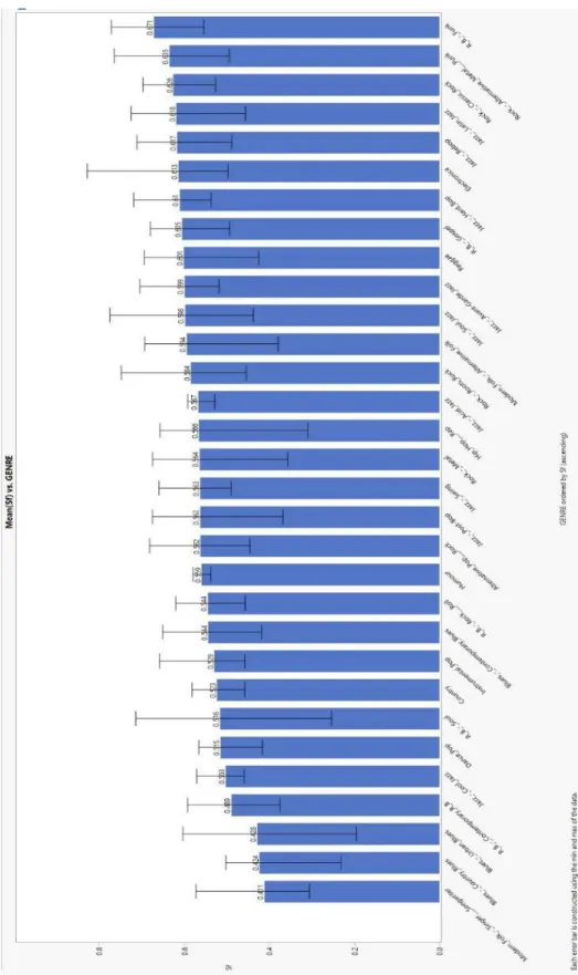
an effect of genre on SF;
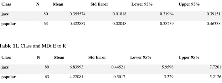
an effect of class on HRt3sF;
an effect of class on MDt from estimations to ground-truth (E to R);
a positive correlation between tempo and SF;
a positive correlation between song duration and MDt R to E;
a negative correlation between song duration and HRt3sF and HRt3sR, but a
positive correlation between song duration and HRt3sP.
a positive correlation between song duration and PWFF and PWFR, but a negative
correlation between song duration and PWFP;
a positive correlation between song duration and SO, but a negative correlation

![Figure 4. The kernel with Gaussian radial function used to measure audio novelty in a self-similarity matrix in [19] and [17]](https://thumb-us.123doks.com/thumbv2/123dok_us/8341867.2215808/18.918.170.443.803.964/figure-kernel-gaussian-radial-function-measure-novelty-similarity.webp)