properties, i.e., increasing data volume and dynamic and evolving nature, mining data streams raised several challenges [6, 7, 8]. The length of data stream would be infinite and an algorithm is needed to process the data in one pass [7, 8]. Therefore, traditional learning algorithms that require several passes on the training data cannot be directly applied to the streaming environment [8, 9]. To solve this problem, ensemble classification techniques have been proposed.
Ensemble approaches have the advantage that they can be updated efficiently, and they can be easily made to adopt the changes in the stream. Several ensemble approaches have been devised for the classification of evolving data streams [10, 11, 12]. The general technique practiced by these approaches is that the data stream is divided into equal-sized chunks. Each of these chunks is used to train a classifier. An ensemble of 𝑀 such classifiers is used to test unlabeled data.
Manual labeling of data is both costly and time-consuming [14, 15]. Therefore, labeled data may be very scared in a real streaming environment, where huge volumes of data appear at high speed. Thus, only a limited amount of training data may be available for building the classification models, leading to poorly trained classifiers [16, 17, 18]. One recently proposed solution to address this issue is to use active learning (AL) techniques which selectively label number of informative instances that can form an accurate predictive model [19, 20, 21]. The goal of active learning is to maximize the prediction accuracy by only labeling a limited number of instances. Meanwhile, the main challenge is about to identify “important” instances that should be labeled to improve the model training due to the fact that one could not afford to label all samples [18]. For example, uncertainty sampling [22, 23], query by committee (QBC) [20] or query by a margin [21] principles takes instances in which the
current learners have the highest uncertainty as the most needed instances for labeling.
Thus, in practice, only small fraction of each data chunk is likely to be labeled, leaving a major portion of the chunk as unlabeled. By only selecting the most informative instances for labeling, active learning could reduce the labeling cost when labeled instances are hard to obtain [24]. Facing the same situation, semi-supervised learning utilizes unlabeled instances to strengthen trained classifiers on labeled instances [25, 26]. In general, active learning methods ignore the effect of unlabeled instances. However, unlabeled instances could strengthen supervised learning tasks under suitable assumptions. A variety of semi-supervised learning methods were proposed based on this idea. Semi-supervised learning methods can be used to strengthen active learners [24, 27, 28]. Therefore, this paper proposed a hybrid method that combines active learning and semi-supervised learning to come up with the mentioned challenges.
In this paper, we present a combination of AL and self-training approach to which we will refer as semi-supervised active learning for data stream mining (SeSAL). To the best of our knowledge, no semi-supervised active learning combination exists for data streams. We introduce minimal variance as a confidence measure in self-training. In multi-class conditions, AL performs better than SeSAL. The nature of Self-training causes this problem. Because of the small initial labeled set, with a high number of classes, self-training weaken itself by generating incorrectly labeled data that redound poor classifier. To avoid such an error propagation, we propose a dynamic self-training algorithm and apply it in our combination framework (DSeSAL). Concerning accuracy reduction in the iterations of self-training algorithm, we indicate a tolerance measure that prevents such downfall, stop
Fig. 1. General process of data stream mining
Input Applying da-ta streams
approaches Output
Data Streams Generators Sensor Networks
Satellites Internet Traffic
Call Records
Data Streams
Knowledge
Selecting Some Part of Data Stream
Preprocessing of Data Streams Incremental Learning Knowledge Extraction
Single Pass
the semi-supervised approach and switch to AL phase. This procedure guarantees to derive a model to predict future instances’ label as accurately as possible.
The rest of this paper is organized as follows: In the next section, related works are reviewed. In Section 3, active learning and semi-supervised learning are recalled as the foundation of our hybrid framework. In Section 4, the proposed framework is presented. Experimental results are reported in Sections 5. Section 6, includes the conclusion.
II.RELATED WORK
In addition to data stream classification, our research is closely related to the existing works on both semi-supervised and active learning. There have been many works in stream data classification. There are two main approaches: single model classification and ensemble classification. Single model classification techniques incrementally update their model with new data to cope with the evolution of the stream [1, 30]. These techniques usually require complex operations to modify the internal structure of the model and may have a poor performance if there is a concept-drift in the stream [4, 31, 32]. In data streams with continuous volumes, the classifier ensemble has shown to be effective in tackling data volume and concept drifting challenges [11, 33, 34]. [30] and [33] proposed a streaming ensemble algorithm that combines decision tree models using majority voting. Kolter and Maloof in [35] proposed an AddExp ensemble method by using weighted online learners to handle drifting concepts. [28, 36] and [37] have proposed a weighted ensemble framework for concept drifting data streams and proved that the error rate of a classifier ensemble is less than a single classifier trained from the aggregated data of all consecutive k chunks. These ensemble approaches have the advantage that they can be more efficiently built than updating a single model and they observe higher accuracy than their single model counterpart [4].
The combination of classifier ensemble and active learning has been reported in much research [19, 39, 40, 41]. Semi-supervised and active learning frameworks concerning data stream classification, are established research areas. Here, some recent and reliable research in this field is introduced. Clustering-training is a semi-supervised framework that select confident unlabeled samples using clustering. Then uses them to retrain the
classifier incrementally which is proposed in [42, 43]. Yan Yu et al. in [44] propose an anomaly detection algorithm for evolving data stream based on semi-supervised learning, SSAD. The SSAD algorithm utilizes an attenuation rule to decrease the effect of historical data on the detection result, which can help the algorithm to learn from current data that characterizes the traffic pattern more accurately. SSAD also uses semi-supervised learning to extend labeled dataset as a training dataset to do with the problem of lack of the labeled data.
Realizing that labeling all stream data is expensive and extremely time-consuming, Fan et al. in [45], proposed an active mining (AM) framework that labels samples only if it is necessary. In short, AM uses a decision tree (trained from the currently labeled data) to compare the distributions of the incoming samples and the data collected by hand using the tree branches (without observing the class labels). If two sets of samples are subject to different distributions, then labeling process is triggered to randomly select a few incoming samples for labeling. Xingquan Zhu et al. in [37] propose a classifier ensemble based active learning framework, with an objective of maximizing the prediction accuracy of the classifier ensemble built from labeled stream data. We use this framework in our method and describe it in more details in the next section.
III.PRELIMINARY
In this section, we recall the two main principles of our hybrid proposed framework: Active learning and Semi-supervised learning.
A. Active Learning
Algorithm 1 describes the general AL framework. A utility function 𝑈𝑀(𝑃𝑖) is the core of each AL approach. It estimates how useful it would be for a specific base learner to have an unlabeled example labeled and, subsequently included in the training set [17].
B. Semi-Supervised Learning
There are many semi-supervised learning methods developed. Self-training learning is the one that needs only one classifier, which is important to meet the speed requirement [28]. We choose Self-training to strengthen the learning engine in AL framework with unlabeled instances. In self-training, first, a classifier is trained with the small amount of labeled data. The classifier is then used to classify the unlabeled data. Typically, the most confident unlabeled points, together with their predicted labels, are added to the training set. The
Algorithm 1 General AL framework Given:
B: number of examples to be selected L: set of labeled examples
P: set of unlabeled examples
UM: utility function
Algorithm:
Loop until stopping criterion is met 1. Learn model 𝑀 from L 2. For all pi∈ 𝑃: 𝑢pi ← 𝑈𝑀(𝑃𝑖)
3. Select B examples pi∈ 𝑃 with highest utility 𝑢pi
4. Query human annotator for labels of all B examples 5. Move newly labeled examples from P to L Return L
Algorithm 2 Self-training Given:
Labeled data {(xi, yi)}i=1l , unlabeled data {xi}j=l+1l+u
Algorithm:
1. Initially, let L = {(xi, yi)}i=1l and U = {xi}j=l+1l+u .
2. Repeat:
3. Train f from L using supervised learning. 4. Apply f to the unlabeled instances in U. 5. Remove a subset S from U; add x, f(x) x ∈ S} to L.
Volume 9- Number 4 – Autumn 2017
classifier is re-trained and the procedure repeated [25, 29]. Note the classifier uses its own predictions to teach it. The overall process of self-training is shown in Algorithm 2.
IV.PROPOSED METHOD
There are two important properties in a real stream environment which lead to many challenges [3]; incremental growth of data volumes and continuous evolvement of decision concepts. In addition, massive volumes of data arrive at high speed, so labeled data may be rare, and it is not possible to manually label all the data as soon as they arrive. In this condition, the best way is to use the advantages of abundant unlabeled data. So, we introduce DSeSAL framework, to
overcome such difficulties and challenges. In this framework, our contributions are as follows:
A. Combination of Active learning and self-training.
B. Introduce minimal variance as a confidence measure in self-training.
C. Propose a dynamic self-training algorithm and combination with active learning.
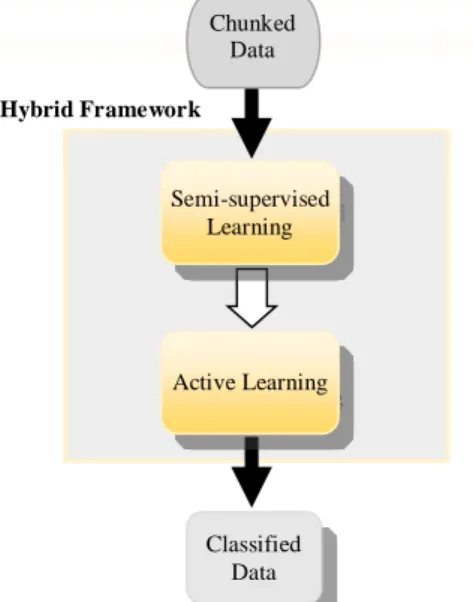
D. Indicate tolerance measure that prevents an accuracy reduction in the iteration of the self-training. We apply semi-supervised learning with active learning in a hybrid manner that benefit from both unlabeled data and selective sampling scenario. The way we combine semi-supervised and active learning is shown in Fig. 2. Naturally, stream data could be stored in the buffer and processed when the buffer is full, so we divide the stream data into equal-sized (user-specified) chunks and exploit our learning process on each of them. Due to the limited number of labeled data in each chunk, we utilize unlabeled data to build a stronger model from each chunk, by applying a semi-supervised approach (Fig. 3).
In order to simplify the problem and deliver an applicable combining framework data streams, we
assume that the concepts in the data are constantly evolving, so the proposed framework is carried out on a regular basis, and the objective is to find important samples out of a certain number of newly arrived instances for labeling.
The proposed framework in Fig. 3 can be applied to a variety of stream applications as long as instance labeling is of concern. The employment of a classifier ensemble ensures that framework can handle massive volumes of stream data effectively and adopt the changes in the stream [1].
Based on the framework in Fig. 3, we assume that once the algorithm moves to chunk Sn, all instances in previous chunks, … , Sn−3, Sn−2, Sn−1, are inaccessible except classifiers built from them (i.e., … , Cn−3, Cn−2,
Cn−1).
Relying on the above assumptions, the objective becomes labeling instances in data chunk Sn such that a classifier Cnbuilt from the labeled and unlabeled instances in Sn. The classifier Cn along with the most recent K − 1 classifiers Cn−k+1, … , Cn−1, can form a classifier ensemble with maximum prediction accuracy on unlabeled instances in Sn.
A. Variance Reduction for Error Minimization In this part, we first argue that minimizing the classifier variance is equivalent to minimizing its error rate and then apply variance as a confidence measure in our semi-supervised approach. In addition, we shortly explain an active learning approach and optimal-weight calculation method that we use in the classifier ensemble.
Confidence measure in self-training
Let x be an input instance and ci is a class label and
p(ci|x) is a classifier’s probability estimation in classifying x, and then the actual probability fci(x) is shown as follows:
where εi(x), is an added error. If we consider that the added error of the classifier mainly comes from two sources, i.e., classifier bias and variance [46, 47, 48], then the added error εi(x) in (1) can be decomposed 𝑓𝑐𝑖(𝑥) = 𝑝(𝑐𝑖|𝑥) + 𝜀𝑖(𝑥) (1)
L U1 1 L U n-k+1 n-k+1 L U n-k+2 n-k+2 L Un n
Input: Data streams (Chunking)
Classifier 1 Cn-k+1 Cn-k+2 Cn Chunkn-k+1
Chunk1 Chunkn-k+2 Chunkn
Classifier Ensemble M
Wn
Wn-k+2
Wn-k+1
W1
Active Learning phase
P
re
d
ictio
n
Semi-Supervised Learning phase
Fig. 2. A general classifier ensemble framework for learning from data streams
Hybrid Framework Chunked
Data
Semi-supervised Learning
Active Learning
Classified Data
Fig. 3. Hybrid of Semi-supervised and Active Learning black box
into two terms, i.e., βci and ηci(x), where βci represents the bias of the current learning algorithm, and ηci(x) is a random variable that accounts for the variance of the classifier (with respect to class ci), which gives [49, 50]:
According to [51], classifiers that trained by using the same learning algorithm but different versions of the training data suffer from the same level of bias but different variance values. Assuming that we are using the same learning algorithm in our analysis, without loss of generality, we can ignore the bias term. Consequently, the learner’s probability in classifying x into class ci becomes:
According to [51] concluded that the classifier’s expected added error can be defined as:
Where p′(. ) denotes the derivate of p(. ) and p(ci|x∗) is the probability distribution of class i for all points x∗, s = p′ c
j|x∗ − p′(ci|x∗), which is independent of the trained model. ηci(x) is a random variable that accounts for the variance of the classifier (with respect to class ci) and ση2ci denotes the variance of ηci(x). As Equation (4) indicates the expected added error of a classifier is proportional to its variance; thus, reducing this quantity reduces the classifier’s expected error rate.
Based on the framework in Fig. 3, we apply variance-base self-training in SSL phase. The main idea is first to train a classifier on labeled data. The classifier is then used to predict the labels for the unlabeled data. A subset of the unlabeled data, jointly with their predicted labels, is then selected to augment the labeled data. Typically, this subset consists of few unlabeled instances with the most confident predictions. The classifier is now re-trained on the larger set of labeled data, and the procedure repeats [43]. We use C4.5 [53] as our base learner. For selecting a subset of unlabeled instances, we use minimum classifier variance on current unlabeled set in each chunk based on Fig. 3. Following above conclusion, smaller variance means the prediction of our model is more confident. In our system, ση2ci is calculated by:
where Λx, an evaluation set (Λx= Ln∪ Îx, where
Îxdenotes Ixwith a predicted class label.), is used to calculate the classifier variance, |Λx| denotes the number of instances in Λx, ycxi is the genuine class
probability of instance x. If x is labeled as classci, then
ycxi is equal to 1; otherwise, it is equal to 0 and fci(x)
denotes the probability of base classifier in classifying x into classci. Consequently, the variance of the classifier over all class c1, c2, … , cl is given by:
Variance and optimal weight classifier ensemble As shown in Fig. 3, k base classifiers form a classifier ensemble M. The probability of the ensemble M in classifying an instance x is given by a linear combination of the probabilities produced by all of its base classifier. Each classifier Cm has a weight value
wm. The probability of M in classifying x into class c i is given by (7), where fcmi(x) denotes the probability of base classifier Cm in classifying x into class ci, i.e.,
This probability can be expresses as:
where ηcEi(x) is a random variable accounting for the variance of the classifier ensemble M with respect to class ci, and
The variance of ηcEi(x) becomes
ση2cim is explained in SSL Phase. The total variance of the ensemble M is then given by:
According to (4), expected added error can be written as:
Equation (12) states that to minimize the error rate of a classifier ensemble, we can minimize its variance instead. This objective can be achieved through the adjustment of the weight value associated with each of 𝑓𝑐𝑖(𝑥) = 𝑝(𝑐𝑖|𝑥) + 𝛽𝑐𝑖+ η𝑐𝑖(𝑥) (2)
𝑓𝑐𝑖(𝑥) = 𝑝(𝑐𝑖|𝑥) + η𝑐𝑖(𝑥) (3)
Erradd=
ση2ci+ ση2cj
s =
σηc 2
s (4)
ση ci E
2 = ∑ (𝑤𝑚)2σ
ηcim 2 𝑛
𝑚=𝑛−𝑘+1
( ∑ 𝑤𝑚
𝑛
𝑚=𝑛−𝑘+1
)
2
⁄ (10)
ση2ci=
1
|Λx| ∑ (yci x − f
ci(x)) 2 (x,c)ϵΛx
(5)
σηc 2 = ∑ σ
ηci 2 l
i=1
(6)
𝑓𝑐𝑖
𝐸(𝑥) = ∑ 𝑤𝑚𝑓
𝑐𝑖 𝑚(𝑥) 𝑛
𝑚=𝑛−𝑘+1 ∑ 𝑤
𝑚 𝑛
𝑚=𝑛−𝑘+1
⁄ = 𝑝(𝑐𝑖|𝑥) + ∑ 𝑤𝑚ηci
m 𝑛
𝑚=𝑛−𝑘+1 ∑ 𝑤
𝑚 𝑛
𝑚=𝑛−𝑘+1
⁄ (7)
𝑓𝑐𝑖
𝐸(𝑥) = 𝑝(𝑐
𝑖|𝑥) + ηci E(x)
(8)
ηcEi= ∑ 𝑤𝑚ηcmi 𝑛
𝑚=𝑛−𝑘+1
∑ 𝑤𝑚
𝑛
𝑚=𝑛−𝑘+1
⁄ (9)
ση2E= ∑ ση ci E
2 l
i=1
= ∑ (𝑤𝑚)2σ ηcm
2 𝑛
𝑚=𝑛−𝑘+1
( ∑ 𝑤𝑚
𝑛
𝑚=𝑛−𝑘+1 )
2
⁄ (11)
ErraddE =
ση2E
S (12)
Volume 9- Number 4 – Autumn 2017
M’s base classifier Cm. In [37], an optimal-weight calculation method is applied to assign weight values to the classifiers such that they can form an ensemble with minimum error rate. To find the weight values wm, m = n − k + 1, … , n , an optimization problem is solved, and then weight values for each individual classifier of the classifier ensemble M are given by:
The minimization of the classifier ensemble error rate through variance reduction acts as a principle to actively select mostly needed instances for labeling.
B. A COMBINED FRAMEWORK OF DYNAMIC
SELF-TRAINING AND ACTIVE LEARNING The process of the DSeSAL method is given in Algorithm 3. Following the conclusions derived from Section IV, we propose a combined framework of AL and SSL approaches for data stream classification. We introduce variance-based self-training. Self-training is characterized by the fact that the learning process uses its own predictions to teach it.
On the other hand, in stream environments, initial labeled data may be very scarce. So, it is conceivable that an early mistake made by the base classifier
(which is not perfect to start with, due to a small initial labeled set) can weaken itself by generating incorrectly labeled data. Re-training with this data will lead to an even worse classifier in the next iteration. It is so expected in multi-class condition. Due to the limited initial labeled set, the base classifier may not be able to identify and learn unseen classes. To alleviate this problem, we propose dynamic self-training, as shown on Steps 5.1 to 5.10 in Algorithm 3.
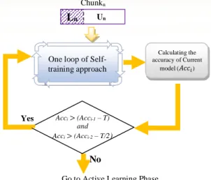
To avoid error propagation in self-training iterations, we specify a tolerance value Τ for accuracy reduction. In our system, Τ is calculated by:
where Accb is the base model accuracy on unlabeled data in the related chunk and Acc1 is the accuracy of the model that build from the first iteration in
self-training. Self-training iterations continue provided: This condition prevents classifier accuracy deterioration and guarantees to derive a model to predict future instances’ label as accurately as possible. The way that the condition in Equation (15) is applied in self-training algorithm, is shown in Fig 4. In Algorithm 3, steps 6 to 11, present the AL procedure.
𝑤𝑚= 1
1 + ση2cm(∑nt=n−k+1,t≠m1 ση c t 2
⁄ ) (13)
𝐴𝑐𝑐𝑖> (𝐴𝑐𝑐𝑖−1− Τ) 𝑎𝑛𝑑 𝐴𝑐𝑐𝑖> (𝐴𝑐𝑐𝑖−2− Τ 2⁄ ) (15)
Τ = | 𝐴𝑐𝑐𝑏− 𝐴𝑐𝑐1| (14)
Input: (1) current data chunk Sn; and (2) 𝑘 − 1 classifiers 𝐶𝑛−𝑘+1, … , 𝐶𝑚, … , 𝐶𝑛−1built from the most recent data chunks;
Parameters: (1) 𝛼, the percentage of instances should be labeled from 𝑆𝑛 by AL; (2) 𝛽; maximum percentage of instances should
be labeled from 𝑆𝑛 by DSSL; (3) 𝛾, # of instances labeled in each SSL iteration
Objective: Updated ensemble 𝑀
1. 𝐿𝑛← ∅; 𝑈𝑛← 𝑆𝑛
2. 𝐿𝑛← Randomly label a tiny portion, e.g. 1~2.5% of instances from 𝑈𝑛.
3. 𝐸 ← 0 //recording the iteration of SSL (E = β γ⁄ ) 4. Build a classifier 𝐶𝑛 from 𝐿𝑛 and calculate the base model accuracy 𝐴𝑐𝑐𝑏.
5. While𝐿𝑛< |𝑆𝑛|. 𝛽 //SSL phase continue until reach the stop point
5.1. For each instance 𝐼𝑥in 𝑈𝑛
a. Use the current classifier to predict a class label for 𝐼𝑥.
b. Build an evaluation set Λ𝑥= 𝐿𝑛∪ 𝐼̂𝑥, where 𝐼̂𝑥denotes 𝐼𝑥with a predicted class label.
c. Calculate the confidence measure (classifier variance) on Λ𝑥(Eqs. (5) and (6)).
End For
5.2. 𝑗 ← 0 // recording the number of labeled instances in each SSL iteration 5.3. Choose instance 𝐼𝑥in 𝑈𝑛with smallest variance, put labeled 𝐼𝑥 into𝐿𝑛, i.e. 𝐿𝑛= 𝐿𝑛∪ 𝐼𝑥; 𝑈𝑛= 𝑈𝑛/𝐼𝑥. 5.4. 𝑗 ← 𝑗 + 1
5.5. If𝑗 < 𝛾
a. Repeat Step 5.3.
5.6. Else
a. 𝐸 = 𝐸 + 1
5.7. Update classifier by a new 𝐿𝑛.
5.8. Calculate the current model accuracy 𝐴𝑐𝑐𝑖. 5.9. If𝐸 = 1
a. calculates the tolerance value Τ (Eq. (11)). 5.10. If 𝐴𝑐𝑐𝑖< (𝐴𝑐𝑐𝑖−1− Τ) 𝑂𝑅 𝐴𝑐𝑐𝑖< (𝐴𝑐𝑐𝑖−2− Τ 2⁄ )
a. Return the model to previous state. b. Return the 𝐿𝑛 and 𝑈𝑛 to previous state.
c. break End While
6. Initialize weight value 𝑤𝑚for each classifier 𝐶𝑚, 𝑚 = 𝑛 − 𝑘 + 1, … , 𝑛, where 𝑤𝑚is equal to 𝐶𝑚’s prediction accuracy on 𝐿𝑛. 7. Use 𝐶𝑛−𝑘+1, … , 𝐶𝑚, … , 𝐶𝑛−1 to form a classifier ensemble 𝑀 as shown in Fig. 1.
8.For each instance 𝐼𝑥in 𝑈𝑛, Calculate ensemble variance (Eq. (11)) as instance 𝐼𝑥’s expected ensemble variance on 𝑀. 9. Choose instance 𝐼𝑥in 𝑈𝑛with largest variance, label 𝐼𝑥and put labeled 𝐼𝑥 into𝐿𝑛, i.e. 𝐿𝑛= 𝐿𝑛∪ 𝐼𝑥; 𝑈𝑛= 𝑈𝑛/𝐼𝑥.
10. Recalculate the ensemble variance of each base classifier 𝐶𝑚on 𝐿𝑛 and find optimum weight value 𝑤𝑚(Eq. (13)) for all base classifiers (update the ensemble by new weight values).
11. Check if α percentages of instances are labeled.
Algorithm 3 The DSeSAL method
Selecting the informative instance and update the ensemble are shown in Steps 6 to 9 and Step 10, respectively.
V.EXPERIMENTAL RESULT A. Implementation
A set of experiments is carried out to compare our algorithm with the results of [37] (MV), random sampling (RS) and uncertainty sampling (US). All methods are implemented in MATLAB with an integration of WEKA data mining tool (Witten, & Frank, 2005). All the tests are conducted on a PC machine with a 2.71GH CPU and 2.0G memory. B. Data Streams
Synthetic data: In order to simulate the magnitude
and speed of concept drift in data streams, a hyper-plane based synthetic data stream generator is applied which is so popular in stream data mining research [11, 12, 33]. The hyper-plane of the data generation is controlled by a non-linear function defined by Equation (16). Given an instance 𝑥, its 𝑓(𝑥) value defined by Equation (16) determines its class label. Assume 𝑓(𝑥) value larger than a threshold 𝜃 indicates that x belongs to class A, otherwise, 𝑥 belongs to class B, then changing the values of ai, 𝑖 = 1, … , 𝑑 and threshold 𝜃 may make an instance 𝑥 have different probability 𝑝(𝑐𝑖|𝑥) with respect to a particular class 𝑐𝑖.
In Equation (16), d is the total dimensions of the input data x. Each dimension xi, i = 1, … , d, is a value randomly generated in the range of [0, 1]. A weight value ai, i = 1, … , d, is associated with each input dimension and the value of ai is initialized randomly in the range of [0, 1] at the beginning. In data generation process, we will gradually change the value of ai to simulate concept drifting. The general concept drifting is controlled through the following three parameters [1, 11, 33]: (1) t, controlling the magnitude of the concept drifting (in every N instances): (2) p, controlling the number of attributes whose weights are involved in the change; (3) h and ni ∈ {−1, 1}, controlling the weight adjustment direction for attributes involved in the
change. After the generation of each instance x, ai is adjusted continuously by ni⋅ t / N (as long as ai is involved in the concept drifting), and value a0 is recalculated to change the decision boundaries (concept drifting). Meanwhile, after the generation of N instances, there is a h percentage of chances that weight change will invert its direction, i.e., ni= −ni for all attributes ai involved in the change. In summary, c2-I100k-d10-p5-N1000-t0.1-h0.2 denotes a two-class data stream with 100k instances, each containing 10 dimensions. The concept drifting involves 5 attributes, and their weights change with a magnitude of 0.1 in every 1000 instances and weight inverts the direction with 20% of chance.
Real-world data: Due to the unavailability of
public benchmark data streams (from classification perspectives), we select five relatively large datasets from UCI data repository [54] and treat them as data streams for our experiments. The datasets we selected are Adult, Magic Gamma Telescope, Covtype, Shuttle and Letter (as listed in Table 1).
Among these datasets, all of them except Letter are considered dense datasets, which means that a small portion of examples can learn genuine concepts quite well. The class distribution in the Covtype and Shuttle datasets are severely biased. Letter is a sparse dataset and 26 classes of examples are evenly distributed, and a small portion of examples are insufficient to learn genuine concepts underlying the data.
C. Evaluation
All results are 10-fold cross-validation accuracies which we set in Weka. C4.5 is our base learner in all experiments.
Learning with Fixed α and β Values: We apply
our proposed framework to two types of synthetic data streams: two-class (Table 2) and four-class (Table 3). The accuracies in the tables denote an ensemble classifier’s average accuracy in predicting instances in the current data chunk Sn, with chunk sizes varying from 250 to 2000. We fix the α and β values to 0.1 and set the k value to 10, which means that 10% of the instances are labeled for each data chunk, and only the
N am e # o f in st an ce s # o f at tri b u te s # o f cla ss es M ajo ri ty : M in o ri ty cla ss ra tio
Adult 48,842 15 2 0.761:0.239
Magic 19,020 10 2 0.351:0.649
Covtype 581,012 55 7 0.488:0.005
Shuttle 58,000 9 7 0.034:0.8
Letter 20,000 17 26 0.041:0.037
f(x) = ∑ ai
xi+ (xi)2 d
i=1 (16)
Table. I. Data characteristics of the real-world data used for evaluation
Fig. 4. Error propagation prevention condition in self-training process
Yes
No
Calculating the accuracy of Current
model (𝐴𝑐𝑐𝑖)
One loop of Self-training approach
Acci > (Acci-1 – T) and Acci > (Acci-2 – T/2)
Go to Active Learning Phase
Ln Un
Chunkn
most recent ten classifiers are used to form a classifier ensemble.
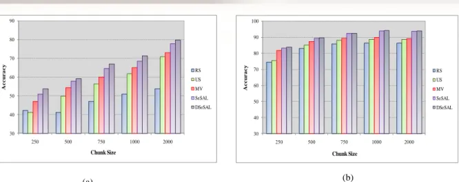
The results from Table 2 and 3 indicate that the performance of all methods deteriorates as a consequence of the shrinking chunk size. This is because a smaller data chunk contains a few examples, and sparse training examples usually produce inferior learners in general. The advantage of having a small chunk size is the training efficiency.
For any particular method, Table 2 and 3 indicate that the results in multi-class data streams are significantly worse than a binary class data stream.
This shows that learning from a multiclass data stream is more challenging than a binary class data stream.
Fig. 5 shows the results from Table 2 and 3 as two histograms. Comparing all five methods, we can easily conclude that SeSAL and DSeSAL receive the best performance across all data streams. The US is not an option for learning from data streams, and its performance is constantly worse than RS regardless of whether the underlying data are binary or multiple classes. The results from RS are surprisingly good, and it is generally quite difficult to beat RS with a substantial amount of improvement.
2) Learning with Different β Value: β is a percentage
of instances should be labeled from Sn by self-training in SeSAL model. In Fig. 6, we compare SeSAL average accuracy w.r.t. different β values on synthetic data.
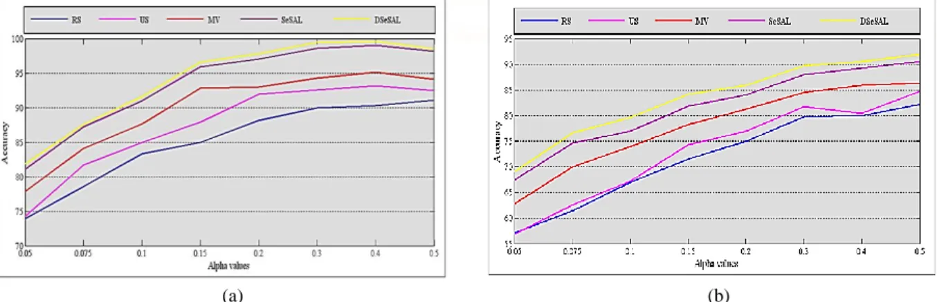
3) Learning with Different 𝛂 Value: In Fig. 7, we
compare all five methods w.r.t. different α values. Not surprisingly, when α value increases, all methods gain better prediction accuracies. This is due to the increasing number of labeled instances helps build strong base classifiers.
Overall, SeSAL, DSeSAL and MV achieve the best performance, and US is inferior to RS in the majority of the cases. For multiclass data streams, the performance of US is unsatisfactory and is largely inferior to the RS. To get the best performance and the lowest cost, we choose 0.1 for α value.
Chunk Size RS US MV SeSAL DSeSAL
250 74.54 75.51 81.84 83.35 84.02 500 83.07 85.16 87.62 89.56 89.79 750 86.10 88.14 89.48 92.63 92.67 1000 86.43 88.79 90.12 94.17 94.37 2000 86.47 88.69 89.16 93.78 94.15
Table. II. Average classification accuracy on c4-I50k-d10-p5-N1000-t0.1-h0.2 (α and β=0.1)
Chunk Size RS US MV SeSAL DSeSAL
250 42.27 41.34 47.21 51.13 53.76 500 50.47 49.91 54.51 57.98 59.24 750 58.11 56.48 60.12 64.63 67.04 1000 63.08 61.92 65.14 68.52 71.51 2000 71.87 70.98 73.09 77.84 79.86
Table. III. Average classification accuracy on c4-I50k-d10-p5-N1000-t0.1-h0.2 (α and β=0.1)
Fig. 6. SeSAL average accuracy on synthetic data (chunk size=500, α=0.1)
30 40 50 60 70 80 90 100
250 500 750 1000 2000
A
c
c
u
r
a
c
y
Chunk Size
RS US MV SeSAL DSeSAL
(b) (a)
30 40 50 60 70 80 90
250 500 750 1000 2000
A
c
c
u
r
a
c
y
Chunk Size
RS US MV SeSAL DSeSAL
Fig. 5. Average classification accuracy histogram on (α and β=0.1): (a) c2-I50k-d10-p5-N1000-t0.1-h0.2, (b) c4-I50k-d10-p5-N1000-t0.1-h0.2
4) Time Complexity and Runtime Performance: The time complexity of the proposed model in Algorithm 3 can be decomposed into two major parts: time complexity of semi-supervised phase and active learning part. As mentioned above, we use MV for Active learning phase. The time complexity of this phase is 𝑂(𝑁2. 𝑀) [37].
same measure (variance) in semi-supervised and active learning phases of the unlabeled instance selection. The total time complexity is bounded by two important factors: 1) the number of instances in each chunk N and 2) the number of data chunks M. Because model training in each chunk is nonlinear w.r.t. the chunk size, we may prefer a relatively small chunk size to save the computational cost.
The time complexity of the semi-supervised part is also O(N2. M), where M is the number of chunks, each of which contains N instances. Because we use the
In Fig. 8, we report the system runtime performance, where the x-axis denotes the chunk size, and the y-axis denotes the average system runtime w.r.t. a single data chunk. Not surprisingly, RS has demonstrated itself to be the most efficient method due to its simple random selection nature. The MV, SeSAL and DSeSAL methods is the most time-consuming approach mainly because the calculation of the ensemble variance and the weight updating requires additional scanning in each chunk. The larger the chunk size, the more expensive the MV, SeSAL, and DSeSAL can be, because the weight we obtain the best
tradeoff between computational cost and accuracy, when the chunk size is 500.
5) SeSAL and DSeSAL Performance on
Real-World Data: For each data stream, we report its results
using chunk size 500. We fix α and β value to 0.1 and set value k to 10, which means that only the most recent 10 classifiers are used to form a classifier ensemble. In Fig. 9, we report the algorithm performances on five real-world data.
According to the results illustrated in Table 4 and Fig. 9, SeSAL provides superior performance than MV on four datasets. These are dense datasets, which means that a small portion of examples can learn genuine concepts quite well. The Letter is a sparse dataset and 26 classes of examples are evenly distributed, and a small portion of examples are insufficient to learn genuine concepts underlying the data. In letter, SeSAL performs inferior to MV in the majority of cases, but DSeSAL solves this problem and provides a reasonable result. The performances of SeSAL and DSeSAL in binary class datasets are close to each other. In fact, DSeSAL eliminates the lack of SeSAL in multi-class problems.
Different from synthetic data streams where the decision concepts in data chunks gradually change following the formula given in Eq. (13), the data chunks of the real-world data do not share such property, and the concept drifting among data chunks are not clear to us (in fact, we do not even know the genuine concepts of the data). Because of this, we compare algorithms on two types of test sets. In Fig. 9,
Table. IV. Average accuracies on real-world datasets
Datasets MV SeSAL DSeSAL
Adult 83.5756 86.0346 86.1398
Magic 79.1676 83.3018 83.7278
Covtype 66.9895 71.3863 78.9498
Shuttle 97.8795 98.8871 99.567
Letter 37.3099 27.9810 47.3161
(a) (b)
Fig. 7. Classification average accuracy on (chunk size=500, β=0.1): (a) c2-I50k-d10-p5-N1000-t0.1-h0.2, (b) c4-I50k-d10-p5-N1000-t0.1-h0.211
Fig. 8. System runtime with respect to different chunk sizes (c4-I50k-d10-p5-N1000-t0.1-h0.2 stream, α and β=0.1) Volume 9- Number 4 – Autumn 2017
the algorithms are tested on all instances in data chunkSn. In Fig. 10, the algorithms are tested on a separate test set generated from 10-fold cross-validation. The x-axis denotes the ratio of the initial labeled set to chunk size.
The results in Figs. 9 and 10 indicate that, overall, the accuracies evaluated on individual data chunks are slightly better than the accuracies acquired from the isolated test set. But overall, an algorithm’s relative performance on each individual data chunk or on a separate test set does not make a big difference.
VI.CONCLUSION
In this paper, we propose a new research topic on the combination of active and semi-supervised learning for data streams with increasing data volumes and evolving nature. Our goal is to derive a model to predict future instances’ label as accurately as possible. In a real stream environment, labeled data may be
fairly scarce and labeling all data is quite difficult and expensive. Active learning and semi-supervised learning are two approaches to alleviate the burden of labeling large amounts of data. We use Active learning and semi-supervised learning to get the advantage of both methods, to boost the performance of learning algorithm.
In our proposed framework, we use self-training with a new confidence measure to take advantage of unlabeled instances to augment the performance of learning algorithm. In multiclass conditions, we face an error propagation and accuracy reduction in SSL phase. To address this problem, we propose a dynamic self-training algorithm (DSeSAL). We control the accuracy reduction by specifying a tolerance measure. Moreover, in our experiments on real data sets, we compared our algorithm with a fully supervised active learning method. The experiments show that the proposed method outperforms the compared methods
.
(a) (b)
(c) (d)
(e)
Fig. 9. Classifier ensemble accuracy on data chunk S¬¬n (chunk size=500, α and β=0.1): (a) Adult ,(b) Magic ,(c) CoverType ,(d) Shuttle ,(e) Letter
References
[1] Domingos, Pedro, and Geoff Hulten. “Mining high-speed data streams.” In Proceedings of the sixth ACM SIGKDD international conference on Knowledge discovery and data mining, 2000, pp. 71-80. ACM.
[2] Han, Jiawei, Jian Pei, and Micheline Kamber. Data mining: concepts and techniques. Elsevier, 2011.
[3] Kholghi, Mahnoosh, Hamed Hassanzadeh, and
MohammadReza Keyvanpour. “Classification and evaluation of data mining techniques for data stream requirements.” In Computer Communication Control and Automation (3CA), 2010 International Symposium on, vol. 1, pp. 474-478. IEEE, 2010.
[4] Masud, Mohammad M., Jing Gao, Latifur Khan, Jiawei Han, and Bhavani Thuraisingham. “A practical approach to classify evolving data streams: Training with limited amount of labeled data.” In Data Mining, 2008. ICDM'08. Eighth IEEE International Conference on, pp. 929-934. IEEE, 2008. [5] Rutkowski, Leszek, Maciej Jaworski, Lena Pietruczuk, and
Piotr Duda. "A new method for data stream mining based on the misclassification error." IEEE transactions on neural networks and learning systems 26, no. 5 (2015): 1048-1059. [6] Aggarwal, Charu C. Data streams: models and algorithms.
vol. 31. Springer Science & Business Media, 2007. [7] Kholghi, Mahnoosh, and Mohammadreza Keyvanpour. "An
analytical framework for data stream mining techniques based on challenges and requirements." arXiv preprint
arXiv:1105.1950 (2011).
[8] Wang, Haixun, Jian Yin, Jian Pei, Philip S. Yu, and Jeffrey Xu Yu. “Suppressing model overfitting in mining concept-drifting data streams.” In Proceedings of the 12th ACM
SIGKDD international conference on Knowledge discovery and data mining, pp. 736-741. ACM, 2006.
[9] Krawczyk, Bartosz, Leandro L. Minku, João Gama, Jerzy Stefanowski, and Michał Woźniak. "Ensemble learning for data stream analysis: a survey." Information Fusion 37 (2017): 132-156.
[10] Yang, Ying, Xindong Wu, and Xingquan Zhu. “Combining proactive and reactive predictions for data streams.” In Proceedings of the eleventh ACM SIGKDD international conference on Knowledge discovery in data mining, pp. 710-715. ACM, 2005.
[11] Gao, Jing, Wei Fan, Jiawei Han, and Philip S. Yu. “A general framework for mining concept-drifting data streams with skewed distributions.” In Proceedings of the 2007 SIAM International Conference on Data Mining, pp. 3-14. Society for Industrial and Applied Mathematics, 2007.
[12] Wang, Haixun, Wei Fan, Philip S. Yu, and Jiawei Han. “Mining concept-drifting data streams using ensemble classifiers.” In Proceedings of the ninth ACM SIGKDD international conference on Knowledge discovery and data mining, pp. 226-235. AcM, 2003.
[13] Brzezinski, Dariusz, and Jerzy Stefanowski. "Combining block-based and online methods in learning ensembles from concept drifting data streams." Information Sciences 265 (2014): 50-67.
[14] Scholz, Martin, and Ralf Klinkenberg. “An ensemble classifier for drifting concepts.” In Proceedings of the Second International Workshop on Knowledge Discovery in Data Streams, pp. 53-64. Porto, Portugal, 2005.
[15] Witten, Ian H., Eibe Frank, Mark A. Hall, and Christopher J. Pal. Data Mining: Practical machine learning tools and techniques. Morgan Kaufmann, 2016.
(a) (b)
(c)
Fig. 10. Classifier ensemble accuracy on a separate test set (chunk size=500, α and β=0.1): (a) Adult, (b) CoverType, (c) Letter
[16] Zhu, Xingquan, and Xindong Wu. “Class noise vs. attribute noise: A quantitative study.” Artificial intelligence review 22, no. 3 (2004): 177-210.
[17] Azimi, Farzaneh, and Karim Faez. "improvement of learning from concept drifting data streams with unlabeled and mixed data."
[18] Rutkowski, Leszek, Maciej Jaworski, Lena Pietruczuk, and Piotr Duda. “A new method for data stream mining based on the misclassification error.” IEEE transactions on neural networks and learning systems 26, no. 5 (2015): 1048-1059. [19] Settles, Burr. “Active learning literature survey.” University
of Wisconsin, Madison 52, no. 55-66 (2010): 11. [20] Settles, Burr. “From theories to queries: Active learning in
practice.” Active Learning and Experimental Design W (2011): 1-18.
[21] Hassanzadeh, Hamed, and Mohammadreza Keyvanpour. "A two-phase hybrid of semi-supervised and active learning approach for sequence labeling." Intelligent Data Analysis 17, no. 2 (2013): 251-270.
[22] Campbell, Colin, Nello Cristianini, and Alex Smola. “Query learning with large margin classifiers.” In ICML, 2000, pp. 111-118.
[23] Aggarwal, Charu C., and S. Yu Philip. "A survey of uncertain data algorithms and applications." IEEE Transactions on Knowledge and Data Engineering 21, no. 5 (2009): 609-623. [24] Muslea, Ion, Steven Minton, and Craig A. Knoblock. “Active
learning with multiple views.” Journal of Artificial Intelligence Research 27 (2006): 203-233.
[25] Huang, Gao, Shiji Song, Jatinder ND Gupta, and Cheng Wu. "Semi-supervised and unsupervised extreme learning machines." IEEE Transactions on Cybernetics 44, no. 12 (2014): 2405-2417.
[26] Imani, Maryam Bahojb, Mohamad Reza Keyvanpour, and Reza Azmi. "Semi-supervised Persian font recognition." Procedia Computer Science 3 (2011): 336-342.
[27] Gadde, Akshay, Aamir Anis, and Antonio Ortega. "Active semi-supervised learning using sampling theory for graph signals." In Proceedings of the 20th ACM SIGKDD international conference on Knowledge discovery and data mining, pp. 492-501. ACM, 2014.
[28] Zhu, Xiaojin, John Lafferty, and Zoubin Ghahramani. “Combining active learning and semi-supervised learning using gaussian fields and harmonic functions.” In ICML 2003 workshop on the continuum from labeled to unlabeled data in machine learning and data mining, vol. 3. 2003.
[29] Chapelle, Olivier, Bernhard Scholkopf, and Alexander Zien. “Semi-supervised learning (chapelle, o. et al., eds.; 2006)[book reviews].” IEEE Transactions on Neural Networks 20, no. 3 (2009): 542-542.
[30] Rutkowski, Leszek, Lena Pietruczuk, Piotr Duda, and Maciej Jaworski. “Decision trees for mining data streams based on the McDiarmid's bound.” IEEE Transactions on Knowledge and Data Engineering 25, no. 6 (2013): 1272-1279. [31] Chandra, Swarup, Justin Sahs, Latifur Khan, Bhavani
Thuraisingham, and Charu Aggarwal. "Stream mining using statistical relational learning." In Data Mining (ICDM), 2014 IEEE International Conference on, pp. 743-748. IEEE, 2014. [32] Zhang, Peng, Xingquan Zhu, and Li Guo. “Mining data
streams with labeled and unlabeled training examples.” In Data Mining, 2009. ICDM'09. Ninth IEEE International Conference on, pp. 627-636. IEEE, 2009.
[33] Street, W. Nick, and YongSeog Kim. “A streaming ensemble algorithm (SEA) for large-scale classification.” In
Proceedings of the seventh ACM SIGKDD international conference on Knowledge discovery and data mining, pp. 377-382. ACM, 2001.
[34] Bose, RP Jagadeesh Chandra, Wil MP Van Der Aalst, Indre Zliobaite, and Mykola Pechenizkiy. "Dealing with concept drifts in process mining." IEEE transactions on neural networks and learning systems 25, no. 1 (2014): 154-171. [35] Kolter, Jeremy Z., and Marcus A. Maloof. “Using additive
expert ensembles to cope with concept drift.” In Proceedings of the 22nd international conference on Machine learning, pp. 449-456. ACM, 2005.
[36] Brzezinski, Dariusz, and Jerzy Stefanowski. "Reacting to different types of concept drift: The accuracy updated ensemble algorithm." IEEE Transactions on Neural Networks and Learning Systems 25, no. 1 (2014): 81-94.
[37] Zhu, Xingquan, Peng Zhang, Xiaodong Lin, and Yong Shi. “Active learning from stream data using optimal weight classifier ensemble.” IEEE Transactions on Systems, Man, and Cybernetics, Part B (Cybernetics) 40, no. 6 (2010): 1607-1621.
[38] Zhu, Xingquan, Xindong Wu, and Qijun Chen. “Eliminating class noise in large datasets.” In ICML, vol. 3, pp. 920-927. 2003.
[39] Melville, Prem, and Raymond J. Mooney. “Diverse ensembles for active learning.” In Proceedings of the twenty-first international conference on Machine learning, p. 74. ACM, 2004.
[40] Mamitsuka, Hiroshi, and Naoki Abe. “Active ensemble learning: Application to data mining and bioinformatics.” Systems and Computers in Japan 38, no. 11 (2007): 100-108. [41] Huang, Shucheng. “An active learning method for mining
time-changing data streams.” In Intelligent Information Technology Application, 2008. IITA'08. Second International Symposium on, vol. 2, pp. 548-552. IEEE, 2008.
[42] Wu, Shuang, Chunyu Yang, and Jie Zhou. “Clustering-training for data stream mining.” In Data Mining Workshops, 2006. ICDM Workshops 2006. Sixth IEEE International Conference on, pp. 653-656. IEEE, 2006.
[43] Xiong, Sicheng, Javad Azimi, and Xiaoli Z. Fern. “Active learning of constraints for semi-supervised clustering.” IEEE Transactions on Knowledge and Data Engineering 26, no. 1 (2014): 43-54.
[44] Yu, Yan, Shanqing Guo, Shaohua Lan, and Tao Ban. “Anomaly intrusion detection for evolving data stream based on semi-supervised learning.” Advances in
Neuro-Information Processing (2009): 571-578.
[45] Fan, Wei, Yi-an Huang, Haixun Wang, and Philip S. Yu. “Active mining of data streams.” In Proceedings of the 2004 SIAM International Conference on Data Mining, pp. 457-461. Society for Industrial and Applied Mathematics, 2004. [46] Friedman, Jerome H. “On bias, variance, 0/1—loss, and the
curse-of-dimensionality.” Data mining and knowledge discovery 1, no. 1 (1997): 55-77.
[47] Moore, David S., and George P. McCabe. Introduction to the Practice of Statistics. WH Freeman/Times Books/Henry Holt & Co, 1989.
[48] RodríGuez, Juan D., Aritz Pérez, and Jose A. Lozano. “A general framework for the statistical analysis of the sources of variance for classification error estimators.” Pattern
recognition 46, no. 3 (2013): 855-864.
[49] Kong, Eun Bae, and Thomas G. Dietterich. “Error-Correcting Output Coding Corrects Bias and Variance.” In ICML, pp. 313-321. 1995.
[50] Tumer, Kagan, and Joydeep Ghosh. “Analysis of decision boundaries in linearly combined neural classifiers.” Pattern Recognition 29, no. 2 (1996): 341-348.
[51] Tumer, Kagan, and Joydeep Ghosh. “Error correlation and error reduction in ensemble classifiers.” Connection science 8, no. 3-4 (1996): 385-404.
[52] Zhu, Xiaojin, and Andrew B. Goldberg. “Introduction to semi-supervised learning.” Synthesis lectures on artificial intelligence and machine learning 3, no. 1 (2009): 1-130. [53] Quinlan, J. Ross. C4. 5: programs for machine learning.
Elsevier, 2014.
[54] Newman, David J., Seth Hettich, Cason L. Blake, and Christopher J. Merz. “{UCI} Repository of machine learning databases.” (1998).
MohammadReza Keyvanpour is an Associate
Professor at Alzahra University, Tehran, Iran. He received his B.S. in software engineering from Iran University of Science & Technology, Tehran, Iran. He received his M. S. and Ph.D. in software engineering from Tarbiat Modares University, Tehran, Iran. His research interests include information retrieval and data mining.
Mahnoosh Kholghi received her B.S. in Software Engineering from Islamic Azad University, Karaj Branch, Karaj, Iran. She also received her M.S. in Software Engineering at Islamic Azad University, Qazvin Branch, Qazvin, Iran. Her research interests include Data Stream Mining and Machine Learning.
Sogol Haghani received her B.S. in computer
science from Kharazmi University, Tehran, Iran. She is currently working toward her master degree in the Department of computer engineering and data mining laboratory at Alzahra University, Tehran, Iran. Her research interests include data mining such as social networks and artificial neural networks. Volume 9- Number 4 – Autumn 2017