Balbeer Singh,1, 2,∗ Lata Thakur,1,† and Hiranmaya Mishra1,‡
1Theory Division, Physical Research Laboratory, Navrangpura, Ahmedabad 380 009, India 2Indian Institute of Technology Gandhinagar, Gandhinagar 382355, Gujarat, India We study the effect of a strong constant magnetic field, generated in relativistic heavy ion collisions, on the heavy quark complex potential. We work in the strong magnetic field limit with the lowest Landau level approximation. We find that the screening of the real part of the potential increases with the increase in the magnetic field. Therefore, we expect less binding of theQQ¯ pair in the presence of a strong magnetic field. The imaginary part of the potential increases in magnitude with the increase in magnetic field, leading to an increase of the width of the quarkonium state with the magnetic field. All of these effects result in the early dissociation ofQQ¯ states in a magnetized hot quark-gluon plasma medium. PACS numbers: 11.10.Wx,14.40.Pq,12.38.Bx,12.38.Mh
Keywords: Heavy quarkonium, Heavy quark-antiquark potential, Dielectric permittivity, Decay width, Debye mass, String tension.
I. INTRODUCTION
Relativistic heavy-ion collisions (RHIC) at Brookhevan and LHC at CERN provide a lot of infor-mation regarding the deconfined state of matter known as quark-gluon plasma (QGP). In recent studies [1] it has been realized that noncentral collisions also produce a strong magnetic field in the direction perpendicular to the reaction plane which has a number of interesting phenomenological consequences [1–5]. The estimated strength of the magnetic field is B =m2π = 1018 Gauss at the RHIC energies andB = 15m2π = 1.5×10¹⁹ Gauss at the LHC energies [1,6], wheremπ is the pion
mass. Possibly, such a huge magnetic field might have existed in the early Universe as an origin of the present large scale cosmic magnetic field [7,8].
The medium in the presence of the magnetic field requires the modification of the existing theo-retical tools that can be used to investigate the various properties of QGP. How the magnetic field modifies the properties of strongly interacting matter has been the subject of various theoretical efforts [9,10]. Various studies, based on direct numerical investigations using lattice QCD [11–13] and effective theoretical investigations using different methods including, e.g., perturbative QCD studies, model studies, and anti-de Sitter/conformal field theory correspondence studies [15–34,74] have predicted many interesting phenomena affecting the properties of strongly interacting mat-ter in the presence of strong magnetic backgrounds. It is still not certain though to what extent such phenomena will be detectable in heavy ion experiments. In this aspect, effects regarding the physics of heavy quark bound states (QQ¯) are of particular interest, since they are more sensitive to the conditions taking place in the early stages. They have large masses and are not affected by the thermal medium. Thus, the heavy quarkonium states are considered as one of the powerful probes to study the deconfining properties of the strongly interacting medium.
Matsui and Satz [35] predicted a suppression of theJ/ψ, being caused by the shortening of the screening length for color interactions in the QGP.
∗
Electronic address: [email protected] †
Electronic address: [email protected] ‡
Electronic address: [email protected]
Initially, it was thought that the large magnetic field produced in such collisions decays very fast [36]. However later, it has been argued that in a medium with finite electric conductivity can sustain strong B-field even in the QGP phase as discussed in Refs. [4,37]. The reason being that the magnetic field does not decay very rapidly due to the induced currents in the medium and satisfies a diffusion equation. Indeed, it is argued that [4, 37] magnetic field decreases fast initially, but at later times, matter effects become more important slowing down the decrease of the magnetic field significantly. This effectively leads to the external magnetic field to be a slowly varying function of time during the entire QGP lifetime.
Simultaneously heavy quark and antiquarks pairs also develop into a physical resonances over a formation timetf orm∼1/Ebind, e.g., thecc¯pairs form resonances at tc¯c∼0.3 fm.
Therefore, it is reasonable to assume that the QQ¯ pair is strongly influenced by the magnetic field. As regards to the effects more directly related to color interactions, various studies have considered the possible influence of an external magnetic field on the static quark-antiquark po-tential [38, 39] and the screening masses [40]. So far, different studies have been carried out on the effects of magnetic field for static properties of quarkonia [38,41–47] and of open heavy flavors [48–52]. The effect of magnetic field on quarkonium production has been discussed in Refs. [43,48]. Further, the influence of strong magnetic field on the evolution ofJ/ψand the magnetic conversion of ηc into J/ψ has been discussed in Refs. [41,53]. Since masses of heavy quarks (mQ) are much
larger than QCD scale (ΛQCD), the velocity v of heavy quarks in the bound state is small, and the binding effects in quarkonia at T = 0 can be understood in terms of nonrelativistic potential models such as Cornell potential which can be derived directly from QCD using the effective field theories (EFTs) [54–56].
In this work we investigate the effects of the magnetic fields on the properties of quarkonium states. Quarkonium states are well understood to be a QQ¯ pair bound by the Cornell potential which is the sum of the Coulombic potential induced by a perturbative one-gluon exchange at short range and linearly rising potential at large distances [57]. In recent years, the quarkonium properties have been investigated by correcting both the Coulombic and string terms of the heavy quark potential through the perturbative HTL dielectric permittivity in both the isotropic and anisotropic medium in the static [58–62] as well as in moving medium [63]. In the present investigation, we focus on the modification of the heavy quark potential in the presence of strong magnetic field.
For the magnetic field considered in the present work , mQ is still the largest scale and the
requirement mQ T and mQ
√
eB is satisfied, so the heavy quark potential can still be described by a nonrelativistic potential. In order to incorporate the magnetic field effect in the heavy quark potential we first calculate the fermionic contribution to the gluon self-energy in the presence of magnetic field in imaginary time formalism by using the Schwinger propagator [64] and calculate the Debye screening mass. Since gluons do not interact with the external magnetic field, the magnetic field dependent contribution arises from the quark loop only. Thus, the total gluon self-energy will be the sum of the gluon (T dependent) and quark (B dependent) loop. As in the deconfined states the gluonic degrees of freedom are larger than the quark degrees of freedom so one must take both of the effects into account to estimate the Debye mass even in the presence of the magnetic field.
In the strong magnetic field approximation only the lowest Landau levels (LLL), which are the energy levels of a moving charged particles, remain active, and the LLL dynamics become important [65]. Therefore, we have taken only the LLL contribution in our calculation. This is a reasonable approximation as quarkonia are produced during the initial stages of collision when the magnetic filed is rather large. Our aim here is to find a field-theory motivated parametrization of the potential that depends both on the temperature and the magnetic field, which will be identified through the Debye screening mass, mD. Further, in the presence of constant magnetic field, the
later, the anisotropic contribution vanishes in the limit of massless light quarks. In this limit the potential remains still isotropic. Here we follow Ref. [66] where the potential is modified by bringing together the generalized Gauss law with the characterization of in-medium effects through the dielectric permittivity. We demonstrate the effect of a strong homogeneous magnetic field on the Debye screening and Landau damping induced thermal width obtained from the imaginary part of the quark-antiquark potential. In the medium, both the perturbative (Coulombic) and nonperturbative (string) part of the heavy quark potential get modified. As the potential is a complex quantity [60,63,67–72] due to which an additional complication will arise. Therefore, a significant description of a relevant physics must illustrate both the effects of Debye screening in the real part of the potential and Landau-damping induced thermal width obtained from the imaginary part of the potential. Recently, the heavy quark potential in a static and strong homogeneous magnetic field has been studied in [73]. However, the authors have studied the effect of magnetic field on the real part of the potential only and they have neglected the gluonic contribution in the Debye mass whereas we have included the gluonic contribution also as discussed above.
This paper is structured as follows. In Sec. II we first calculate the gluon self-energy using the imaginary time formalism and then calculate the Debye mass by taking the static limit of self-energy. In Sec.IIIwe discuss the heavy quark complex potential in the presence of magnetic field and shows the variation of the real and imaginary parts of the potential with the various values of magnetic field at different temperatures. In Sec.IV we investigate the decay width and discuss its variation with the magnetic field for both bottomonium and charmonium ground states. Finally, we present our conclusion in Sec.V.
II. GLUON SELF-ENERGY IN LLL IN THE PRESENCE OF MAGNETIC FIELD In this section we evaluate the one loop gluon self-energy arising from quark loops which gets modified in the presence of the magnetic field. We shall use it to estimate the Debye screening mass for the gluons defined through the vanishing four momentum of the polarization tensor. Moreover, we shall also use the momentum dependent polarization function to estimate the permittivity of the medium which will be used later to estimate the heavy quark potential. We note that such a calculation for the Debye mass for the photons was carried out in Refs.[51, 74, 75]. In the following, we briefly outline the calculations as in Ref.[75] taking care of the appropriate color factors. Consider that a charged particle of chargeqf and massmf is moving in a constant magnetic
field (B) which is acting along the z-direction, i.e.,B~ =Bzˆ. In this scenario the propagator of the charged particle is a function of both the transverse and longitudinal component of the momentum ( with respect toB), which is due to the breaking of Lorentz invariance.
The fermion propagator in coordinate space is written as [64]
S(y, y0) = Φ(y, y0)
Z d4k (2π)4e
−ik·(y−y0)
S(K), (1)
where Φ(y, y0) is the phase factor and can be gauged away. In Eq. (1), S(K) is the Fourier transform of the fermion propagator. It is convenient to write the propagator in the Landau level representation. Proceeding in a similar way as done in Ref. [76] for Euclidean space, the resulting propagator can be written as
S(K) =−ie− K2 ⊥ qf B ∞ X l=0 (−1)lDl(qfB, K) Kk2+m2f + 2l|qfB| , (2)
where the sum is over all the Landau levels (l= 0,1,2,....), and Dl(qfB, K) = (mf−K/k) (1 +iγ1γ2)Ll 2K2 ⊥ qfB −(1−iγ1γ2)Ll−1 2K2 ⊥ qfB + 4K⊥L/ 1l−1 2K2 ⊥ qfB , (3)
whereKk = (K4, K3),K⊥= (K1, K2) are the 4-momentum component parallel and perpendic-ular to the magnetic field with K4 =−iK0 and γ1, γ2 are the Dirac matrices.
The energy spectrum of a charged fermion in the presence of magnetic field can be written as [77] El2(K3) =K32+m2f + 2l|qfB|, (4)
which can be obtained from Eq. (2) by equating the denominator of the propagator to zero. From Eq. (4), it is clear that the energy of fermion is discrete in the direction perpendicular to B and continuous in the direction parallel to the magnetic field. The discretization of energy levels is known as Landau levels.
In the presence of a very strong magnetic field, i.e., qfB T2 the higher Landau levels (l1)
are at infinity as compared to LLL [75, 78] due to which the LLL dominates and the dimensional reduction takes place. For LLL approximation one can use the relations Ln(x) = L0n(x) and
Lα−1(x) = 0 (by definition). In this approximation, the fermion propagator Eq. (2) becomes
S(K) =ie− K2⊥ qf B K/ k−mf Kk2+m2f (1 +iγ1γ2), (5)
where the factor (1+iγ1γ2) is the projection operator which appears because the spin of the fermion in the LLL is polarized parallel to the magnetic field hence signifies the spin-polarized nature of LLL [10]. The spin orientation is parallel/antiparallel to the magnetic field direction for the positively/negatively charged fermion. The form of the propagator in Eq. (5) clearly demonstrates the dimensionally reduced character (1 + 1) of the LLL. It is evident that the dimensional reduction restricts the motion of charged particles perpendicular to the magnetic field.
For evaluating the gluon polarization tensor and Debye screening mass we use the following identities
bµk = (b4,0,0, b3); a2k =a24+a23; b
µ
⊥ = (0, b1, b2,0), (a·b)k=a4b4+a3b3; (a·b)⊥=a1b1+a2b2,
where k and ⊥ are the parallel and perpendicular components. In a background magnetic field, the only contribution to the gluon self-energy comes from the quark loop as shown in Fig. 1. As gluons do not interact with the magnetic field so their contribution remains the same as that at B = 0.
Therefore, the quarks contribution to the gluon self-energy in the presence of magnetic field, δΠµν(P, B) can be written as δΠµν(P, B) = Z d4K (2π)4T r[(gt aγ µ)S(K)(gtbγν)S(K−P)], (6)
where S(K) is fermion propagator as defined in Eq. (5). As the dimensional reduction separate the parallel and perpendicular component of the momentum in the propagator. So the self-energy can
K
−
P
K
P
P
FIG. 1: Gluon self-energy in the presence of strong magnetic field .
also be separated into components. The perpendicular part of the self energy in Eq. (6) is written as I⊥ = 1 (2π)2 Z ∞ −∞ Z ∞ −∞ dKxdKyexp[ 1 qfB (−Kx2−(Kx−Px)2)] exp[ 1 qfB (−Ky2−(Ky−Py)2)] = X f πqfB 2(2π)2 exp −P2 ⊥ 2qfB . (7)
Therefore, Eq. (6) becomes δΠµν(P, B) =g2T r(tatb)I⊥ Z d2K k (2π)2 T r[γµ(K/k−mf)(1 +iγ1γ2)γν((K/ −P/)k−mf)(1 +iγ1γ2)] (K2 k +m2f)((K−P)2k+m2f) . (8) In the imaginary time formalism, the temporal component of self energy becomes
δΠ44(P, B) =g2T r(tatb)I⊥ Z dK 3 (2π)T X n 8ωn2 −8K32−8m2f −8ωnω+ 8K3P3 (ω2 n+K32+m2f)((ω−ωn)2+ (K3−P3)2+m2f) , (9) where ωn= (2n+ 1)πT is fermionic Matsubara frequency and ω is bosonic Matsubara frequency.
For massless fermion (mf = 0) we get
δΠ44(B) = 8g2T r(tatb)I⊥ Z dK 3 (2π)T X n ˜ ∆(K)−(2K32+ωnω−K3P3) ˜∆(K) ˜∆(K−P) , (10) where ˜∆(K) = 1 ω2 n+K23 , ˜∆(K−P) = (ω−ω 1
n)2+(K3−P3)2. In order to calculate the Debye screening mass one can take the static limit of temporal component of self-energy, Π44viz. m2D =−Π44(ω→
0,P~ = 0). After taking the static limit Eq. (10) becomes δΠ44(B)|(ω→0, ~P=0) = 8g2T r(tatb)I⊥ Z dK 3 (2π)T X n ˜ ∆(K)−2K32( ˜∆(K))2 (11) After doing the sum over Matsubara frequency mode in Eq. (11) as in Refs. [75, 79], one can get δm2D = 4g2βI⊥ Z dK 3 (2π) ˜ f(E)(1−f˜(E)). (12)
By using Eq. (7), the Debye screening mass in the presence of the magnetic field becomes δm2D =X f |qf|Bg2 πT Z ∞ 0 dK3 2π ˜ f(E)(1−f˜(E)). (13) By taking the gluonic contribution into account the total Debye mass becomes
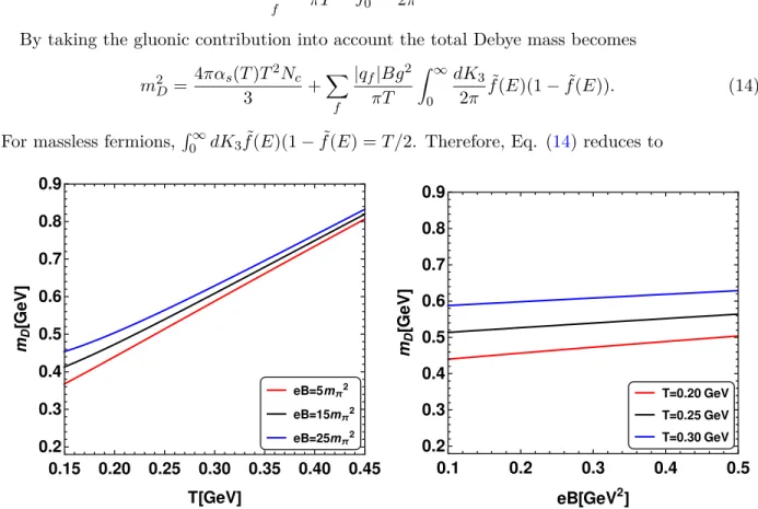
m2D = 4παs(T)T 2N c 3 + X f |qf|Bg2 πT Z ∞ 0 dK3 2π ˜ f(E)(1−f˜(E)). (14)
For massless fermions, R∞
0 dK3f˜(E)(1−f˜(E) =T /2. Therefore, Eq. (14) reduces to
eB=5mπ2 eB=15mπ2 eB=25mπ2 0.15 0.20 0.25 0.30 0.35 0.40 0.45 0.2 0.3 0.4 0.5 0.6 0.7 0.8 0.9 T[GeV] mD [ GeV ] T=0.20 GeV T=0.25 GeV T=0.30 GeV 0.1 0.2 0.3 0.4 0.5 0.2 0.3 0.4 0.5 0.6 0.7 0.8 0.9 eB[GeV2] mD [ GeV ]
FIG. 2: Left panel: Variation of the Debye screening mass (mD) with temperature for different values of magnetic field (eB). Right panel: Variation ofmD with magnetic field for different values ofT.
m2D = 4παs(T)T 2N c 3 + X f |qf|Bαs(T) π . (15)
whereαs(T) is the one loop coupling constant and which can be written as
αs(T) = gs2(T) 4π = 6π (33−2Nf) ln 2πT ΛMS . (16)
Here we useNf = 3 and ΛMS= 0.176 GeV [80].
In the left panel, Fig. 2 shows the variation of Debye screening mass for mf = 0 with T for
different values of magnetic field, i.e.,eB= 5m2π, 15m2πand 25m2π, respectively. In the right panel, the figure shows the variation of Debye screening mass withB for different values of temperature, i.e.,T = 0.20, 0.25 and 0.30 GeV, respectively. Here the Debye screening mass Eq. (15) depends on the two scales, i.e.,T andB. We find that the Debye screening mass increases with the increase in temperature and magnetic field in a magnetized hot QCD medium. Indeed, the effect of magnetic field is stronger at a lower temperature and becomes weaker at a higher temperature. Therefore, we can say that there is a finite amount of Debye screening withT andB formf = 0. The observed
increase of screening mass as a function of magnetic field is in qualitative agreement with lattice QCD computation [40].
III. IN-MEDIUM HEAVY QUARK POTENTIAL IN MAGNETIC FIELD
In this section we study the modification of the Cornell potential in the presence of a hot medium endowed also with a magnetic field. Before that let us first discuss the heavy quark-antiquark potential for a vanishing magnetic field. Consider that a test charged particle is placed at the origin and an auxilar vector field due to this is written as E~ = qrb−1ˆr, where b is a parameter that can have any value. The corresponding potential can be defined by using the relation -∇~V(r) =E~(r). Therefore, the Gauss law can be defined as [66,81]
~ ∇. E~ rb+1 = 4πqδ(r). (17)
As per the Debye-H¨uckle framework, the medium gets polarized and leads to a change of the source term on the right hand side of Eq. (17) fromδ(r) toδ(r) +hρ(r)i. Herehρ(r)iis the induced charged density and can be written in the Boltzmann’s distribution as the difference of the particle and antiparticle charge deviation. At high temperatures and weak potential the charge density can be approximated as hρ(r)i=−2qβn0V(r), which is equivalent to the linear response approxima-tion. Hereβ = 1/T and n0 is the charge density in the absence of test charge. After substituting the above relation into Eq. (17) and by choosing the appropriate values ofband q, one can obtain the Coulombic and string part of the potential. For b =−1, q = α(= αsCF = g
2
sCF
4π ;CF = 4/3),
Eq. (17) reduces to the Coulomb potential and and for b = 1, q = σ, one can obtain the linearly rising (string part) potential, where σ is the string tension and αs is the QCD running coupling.
The detailed calculation of the potential for finite T in the Debye-H¨uckel approach can be found in Ref. [66].
In a quantum field theory framework, the medium effects, i.e., the effect of finite temperature and magnetic field can be incorporated by modifying the vacuum potential with dielectric permittivity as in Ref. [60]. The in-medium permittivity (~p, mD) can be written as
−1(~p, mD) =−lim ω→0p
2D00(ω, p) . (18)
whereD00 is the gluon propagator calculated from the gluon self energy. This will have contribu-tions from the gluonic and fermionic loop. We evaluate each of the contribucontribu-tions in the presence of magnetic field in the following way.
A. Gluon contribution
As the gluonic contribution does not depend upon the magnetic field, the longitudinal part of the gluon self-energy can be written as [82]
δΠL(ω, p)g=m2Dg 1− ω 2pln ω+p ω−p +iπω 2pθ(p 2−ω2) (19) wherem2
Dg= 13g2T2Nc and θ(p2−ω2) is the step function. In the above equation, the imaginary part is related to the Landau damping, which corresponds to the emission and absorption of particle in the medium.
B. Fermion contribution
From Eq. (9), we can get δΠL(ω, p) ≡ δΠ44(ω, p) after doing sum over fermionic Matsubara frequencies. There are two types of frequency sum in Eq. (9) which we evaluate here in detail. The first type is given by
TX n 1 (ω−ωn)2+EQ2 = TX n 1 2EQ 1 EQ+i(ω−ωn) − 1 EQ−i(ω−ωn) = 1 4EK tanh E K−ω 2T + tanh E K+ω 2T (20) and the second type is
TX n 1 ((ω−ωn)2+EQ2)(ω2n+EK2 ) = TX n 1 4EKEQ 1 (EK+iωn)(EQ+i(ω−ωn)) + 1 (EK−iωn)(EQ+i(ω−ωn)) + 1 (EK+iωn)(EQ−i(ω−ωn)) + 1 (EK−iωn)(EQ−i(ω−ωn)) . (21)
Using the summation over the discrete Matsubara frequencies (ωn = (2n+ 1)πT) above equation
becomes TX n 1 ((ω−ωn)2+EQ2)(ω2n+EK2 ) = 1 4EQEK f˜(E K)−f˜(EQ−ω) ω+EK−EQ + ˜ f(EK)−f˜(EQ+ω) EK−EQ−ω + 1− ˜ f(EK)−f˜(EQ−ω) EK+EQ−ω +1− ˜ f(EK)−f˜(EQ+ω) EK+EQ+ω . (22) In the above, the expressions are written after doing an analytic continuation to Minkowski space. The imaginary part of the longitudinal component of the self-energy for fermion loop (=δΠ44) can be calculated by using the identity
=δΠL(ω, p)f = 1 2iηlim→0 δΠL(ω+iη, p)−δΠL(ω−iη, p) (23) along with the expression
1 2i 1 ω+P jEj+iη − 1 ω+P jEj −iη =−πδ(ω+X j Ej). (24)
Using Eqs. (20) and (22) in Eq. (9) the imaginary part ofδΠL reduces to
δ=ΠL(ω, p)f = −π4g2I⊥ Z dK 3 2π −2K2 3+K3P3+ 2m2f 4EQEK (−f˜(EK) + ˜f(EQ−ω)) × δ(ω+EK−EQ) + ( ˜f(EK)−f˜(EQ+ω))δ(ω−EK+EQ) + (1−f˜(EK) − f˜(EQ−ω))δ(EK+EQ−ω) + (1−f˜(EK)−f˜(EQ+ω))δ(EK+EQ+ω) . (25)
In the limit ω → 0, the third and fourth terms will vanish. Therefore, the above equation becomes δ=ΠL(ω, p)f|ω→0 =πω4g2 Z dK 3 2π −2K2 3+K3P3+ 2m2f 4EQEK ∂f(E Q) ∂EQ δ(EK−EQ). (26)
Here, the integral can be solved by using the properties of the Dirac delta function as δ(f(x)) =X
n
δ(x−xn)
|∂f∂x(x)|x=xn
(27)
wherexn are the zeros of the functionf(x). In Eq. (25) delta functions give zeros as
K30= 4P3(P32−ω2)± q 16P2 3(P32−ω2)2−16(P32−ω2)((P32−ω2)2−4m2ω2) 8(P2 3 −ω2) (28) In the limit ω→0, we have only one zero of the function, K30=P3/2, so that
=δΠL(p) = ωβg 2m2 fI⊥ P3E ( ˜f(E)−f˜2(E)) (29) whereE = r m2f +P32
4 . For calculating the fermion loop contribution to the imaginary part of the gluon propagator, we use the spectral function approach in which the propagator is related to real and imaginary parts of the self-energy, it can be written as [83]
=Dµν(ω, P) =−π(1 +e−βω)ξµν. (30)
Here, we focus only on DL≡D00, for this purpose we writeξ00 as
ξ00(ω, P) = 1 π
eβω
eβω−1ρL(ω, P) (31)
whereρL is the longitudinal part of spectral function which describes the quasiparticles with finite
width. In Breight-Wigner form it is written as ρL(ω, P) =
=ΠL
(P2− <Π
L)2+=ΠL2
. (32)
Taking fermion and gluon contributions into account, real and imaginary parts of self-energy can be written as
<ΠL(ω, p) =<ΠL(ω, p)g+<ΠL(ω, p)f, (33)
=ΠL(ω, p) ==ΠL(ω, p)g+=ΠL(ω, p)f. (34)
Here,<ΠL is the real part of the longitudinal component of self-energy, which is the square of the Debye screening mass (m2D) in the limitω→0, (Eq. (15)).
Therefore, using the expression for real and imaginary parts of the self-energy in the limit ω→0, we have calculated the gluon propagator (D00) in terms of real and imaginary parts as
D00(p) = −1 p2+m2 D + iπT m 2 Dg p(p2+m2 D)2 − i|qfB|m 2 fαs 2(p2+m2 D)2P3Ecosh2(βE2 ) . (36)
Note that due to the specific direction of the magnetic field the contribution of the fermion field loop makes the propagator anisotropic. However, in the limit of vanishing light quark mass the propagator remains still isotropic with the effect of magnetic field showing only in the Debye mass. Thus, the dielectric permittivity can be calculated from Eq. (18) and in the limit of massless fermions, it becomes −1(~p, mD) = p2 p2+m2 D −iπT pm 2 Dg (p2+m2 D)2 . (37)
From the above equation it is clear that the permittivity is isotropic in the limit of vanishing light quark masses. Further, for an effective description of quarkonium in terms of a potential at finite temperature, the mass of heavy quark , mQ should be much larger than ΛQCD as well as
mQ T. For the magnetic field considered here, mQ is still the largest scale (mQ
√
eB) i.e., the ratio,m2Q/eB '3−15 for the range of magnetic field eB= 5−25m2π, so that the interaction between quark and antiquark can be described by a quantum mechanical potential. Therefore, our approximation to take the static heavy quark potential for heavy quarkonia should be valid here. This has been attempted here to obtain the effects of the medium on the vacuum potential by correcting both the short and long distance part by a dielectric function encoding the effects of the magnetized deconfined medium.
The Coulomb part of the potential in Fourier space in the presence of medium can be written as [84]
k2VC(~p) = 4π
α (~p, mD)
(38) The Fourier transformation of Eq. (38) in coordinate space gives
− ∇2VC(r) +m2DVC(r) =α(4πδ(r)−iT m2Dgh(mDr)) (39) whereh(y) = 2R∞ 0 dx x (x2+1) sin(yx) yx .
In a similar manner, one can calculate the string part of the potential and get the differential equation for VS(r) as [66] − 1 r2 d2VS(r) dr2 +µ 4V S(r) =σ(4πδ(r)−iT m2Dgh(mDr)), (40) whereµ= (m 2 Dgσ α )1 /4.
After using the boundary conditions mD → 0,<VC(r) =−αr and r → 0,=VC(r) = 0 [85], one
can obtain both the real and imaginary part of the Coulomb potential as
<VC(r, T, B) =−α
e−mDr
r −αmD, (41)
and
where g(y) =R∞
0 dx(x2+1)x 2
1−sin(yxyx)
. Thus, the magnetic field dependence of the potential arises from the field dependent Debye mass.
Similarly, for the string part of the potential we use the following boundary conditions µ →
0,<VS(r) =σr,r →0,=VS(r) = 0 and r → ∞,d=VdrS(r) = 0. After using the boundary conditions
we get both the real and imaginary parts of string potential as
<VS(r, T, B) =− Γ(14) 234 √ π σ µD−12( √ 2µr) + Γ( 1 4) 2Γ(34) σ µ, (43)
whereDν(x) is the parabolic cylinder function, and
=VS(r, T, B) =− σm2DgT µ φ(µr), (44) where φ(µr) = D−1 2 (√2µr) Z r 0 dx<D−1 2 (i√2µx)x2g(mDx) +<D−1 2 (i√2µr) Z ∞ r dxD−1 2 (√2µx)x2g(mDx) − D−1 2 (0) Z ∞ 0 dxD−1 2 (√2µx)x2g(mDx),
The total real part of the potential after combining both the Coulombic and string parts in a magnetized medium can be written as
<V(r, T, B) = <VC(r, T, B) +<VS(r, T, B) = −αe −mDr r −αmD− Γ(14) 234 √ π σ µD−12 (√2µr) + Γ( 1 4) 2Γ(34) σ µ. (45)
Similarly, the total imaginary part of the potential becomes
=V(r, T, B) = =VC(r, T, B) +=VS(r, T, B)
= −2αT g(mDr)−
σm2DgT
µ φ(µr), (46)
In the framework of Debye-H¨uckel theory, the Coulomb and string terms were modified with different screening scalesmDandµ, respectively, to obtain the heavy quark potential. On the other
hand in Ref. [73] the authors have used the same screening scale,mD for both the Coulombic and
linear terms. It is interesting to see the effects of different scales for the Coulombic (perturbative) and the linear (nonperturbative) terms.
Figure 3 shows the variation of the real part of the potential with the separation distance (r) between the Q ¯Qpair for different values of magnetic field (eB= 5m2π, 15m2π, 25m2π ) atT = 200 MeV (left) and T = 250 MeV (right). Here, we use the value of the string tension, σ = 0.174 GeV2 from Ref. [66] . From the figure we find that the screening increases with the increase in magnetic field. The screening is more at a higher temperature (T = 250 MeV) as compared to lower temperature (T = 200 MeV) because at higher temperatures the quarkonium state is loosely bound as compared to the lower temperatures and gets easily dissociated. Alternatively, we can say that with the increase in temperature the gluonic contribution becomes more which results in more screening.
Figure4shows the variation of the imaginary part of the potential with the separation distance (r) for various values of magnetic field ( eB = 5m2π, 15m2π, 25m2π ) at temperatures T = 200
eB=5mπ2 eB=15mπ2 eB=25mπ2 0.5 1.0 1.5 2.0 -0.2 -0.1 0.0 0.1 0.2 0.3 r[fm] ReV [ GeV ] T=200 MeV eB=5mπ2 eB=15mπ2 eB=25mπ2 0.5 1.0 1.5 2.0 -0.2 -0.1 0.0 0.1 0.2 0.3 r[fm] ReV [ GeV ] T=250 MeV
FIG. 3: Variation of the real part of potential with separation distancerbetweenQQ¯ for various values of magnetic field atT = 200 MeV (left) andT = 250 MeV (right).
eB=5mπ2 eB=15mπ2 eB=25mπ2 0.2 0.4 0.6 0.8 1.0 -0.14 -0.12 -0.10 -0.08 -0.06 -0.04 -0.02 r[fm] ImV [ GeV ] T=200 MeV eB=5mπ2 eB=15mπ2 eB=25mπ2 0.2 0.4 0.6 0.8 1.0 -0.14 -0.12 -0.10 -0.08 -0.06 -0.04 -0.02 0.00 r[fm] ImV [ GeV ] T=250 MeV
FIG. 4: Variation of the imaginary part of the potential with the separation distance,r for various values of magnetic field atT = 200 MeV (left) andT = 250 MeV (right).
MeV and T = 250 MeV. We find that the imaginary part of the potential increases in magnitude with the increase in magnetic field and hence it contributes more to the Landau damping induced thermal width obtained from the imaginary part of the potential. The increase in the magnitude of the imaginary part of the potential is more at a higher temperature (T = 250 MeV) as compared to a lower temperature (T = 200 MeV) for a given r.
IV. DECAY WIDTH
The decay width (Γ) can be calculated from the imaginary part of the potential. The following formula gives a good approximation to the decay width of QQ¯ states [60,63,86]
Γ =− Z
d3r|ψ(r)|2=V(r, T, B) (47) whereψ(r) is the Coulombic wave function for the ground state and is given by
ψ(r) = q1 πa3
0
e−r/a0, (48)
wherea0 = 2/(mQα) is the Bohr radius of the heavy quarkonium system. We use the Coulomb-like
wave functions to determine the width since the leading contribution to the potential for the deeply bound quarkonium states in a plasma is Coulombic.
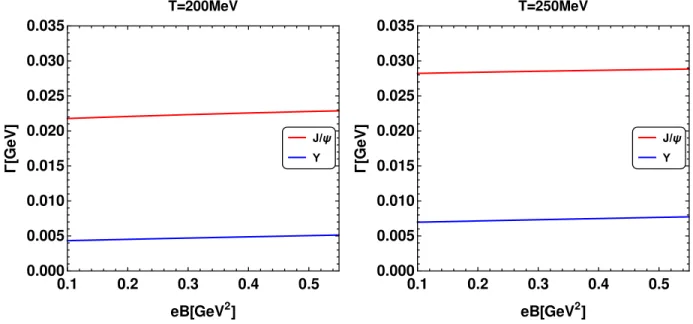
J/ψ Υ 0.1 0.2 0.3 0.4 0.5 0.000 0.005 0.010 0.015 0.020 0.025 0.030 0.035 eB[GeV2] Γ [ GeV ] T=200MeV J/ψ Υ 0.1 0.2 0.3 0.4 0.5 0.000 0.005 0.010 0.015 0.020 0.025 0.030 0.035 eB[GeV2] Γ [ GeV ] T=250MeV
FIG. 5: Variation of decay width with the magnetic field forJ/ψand Υ atT = 200 MeV (left) andT = 250 MeV (right)
.
After substituting the expression for the imaginary part of the potential as given in Eq. (46), in Eq. (47) we estimate numerically the decay width for given T and B. In Fig. 5 we show the variation of decay width for the ground states of charmonium and bottomonium atT = 200 MeV (left panel) andT = 250 MeV (right panel). Here we take charmonium and bottomonium masses as mc = 1.275 GeV and mb = 4.66 GeV respectively from Ref. [87]. We find that the thermal
width increases with the increase in magnetic field. The width for the Υ is much smaller than the J/ψbecause the bottomonium states are smaller in size and larger in masses than the charmonium states and hence get dissociated at higher temperatures. The width at a higher temperature (T = 250 MeV) is more as compared to a lower temperature (T = 200 MeV) for bothJ/ψand Υ. Alternatively, we can say that the Γ increases with the increase in magnetic field which results in the early dissociation of quarkonium states.
Figure. 6shows the variation of the ratio of the decay width [Γ(B = 0)−Γ(B = 0)/Γ(B = 0)] with magnetic field atT = 200 and T = 250 for J/ψ. From the figure it is clear that the change
T=250 MeV T=200 MeV 0.1 0.2 0.3 0.4 0.5 0.00 0.05 0.10 0.15 0.20 0.25 eB[GeV2] [ Γ ( B )-Γ ( B = 0 )] / Γ ( B = 0 ) J/ψ
FIG. 6: Variation of the ratio of decay width [Γ(B)−Γ(B = 0)/Γ(B = 0)] with magnetic field forJ/ψ at
T = 200 andT = 250
.
in decay width for T = 200 MeV is about 11% foreB '5m2
π to as large as 14% for eB '25m2π.
For T = 250, the change is from 5% to 7% in the same range of magnetic field. The magnetic field effects become weaker at a high temperature as compared to a low temperature. Also, we are considering the strong field LLL approximation, i.e.,eB T2. This approximation may not hold good at a high temperature.
V. CONCLUSION
In this work we have studied the effect of a strong magnetic field on the heavy quark com-plex potential in a thermal QGP medium. In order to incorporate the magnetic field effect in the heavy quark potential we first calculated the gluon self-energy in the imaginary time formalism by using the Schwinger propagator in the presence of the magnetic field and then calculated the Debye screening mass (mD). We have shown the variation of Debye mass with magnetic field and
temperature for massless fermions. We found that Debye screening increases in a hot magnetized medium. We have taken only the LLL contribution in our calculation. This is a reasonable approx-imation as quarkonia are produced during the initial stages of collision when the magnetic field is very high and the higher Landau levels are at infinity as compared to LLL due to which the LLL dominates and the dimensional reduction takes place. Further, we study the magnetic field effects on the heavy quark complex potential. This is attempted here through estimating the permittivity of the medium using imaginary time formulation. The presence of magnetic field results is an anisotropic contribution to the gluon propagator from the quark loop. However, such an effect vanishes in the limit of massless quarks and the potential remains isotropic even in the presence of the magnetic field. The effect of the magnetic field in the LLL approximation is manifested through the Debye mass. The heavy quark complex potential is obtained by bringing together the generalized Gauss law with the characterization of in-medium effects, i.e., finite temperature and magnetic field, through the dielectric permittivity. Because of the heavy quark mass (mQ ), the
requirementmQT and mQ
√
eB is satisfied for the range of magnetic fieldeB = 5−25 m2π. We have shown the effect of magnetic field on the Debye screening and Landau damping induced thermal width obtained from the imaginary part of the quark-antiquark potential. In order to see the magnetic field effect on the screening we first show the effect of magnetic field on the real part of the potential. We found that the real part of the potential decreases with increase in magnetic field and becomes more screened. The screening also increases with the increase in temperature. Since the QQ¯ potential is effectively more screened in the presence of magnetic field which results in the earlier dissociation of quarkonium states in a strongly magnetized hot QGP medium.
We have also shown the effect of magnetic field on the imaginary part of the potential and hence on the thermal width. The imaginary part of the potential increases in magnitude with the increase in magnetic field and temperature. As a result, the width of the quarkonium states (J/ψ and Υ ) get more broadened with the increase in magnetic field and results in the earlier dissociation of quarkonium states in the presence of magnetic field. The width for Υ is much smaller than the J/ψbecause bottomonium states are tighter than the charmonium state and hence get dissociated at a higher temperature. We found a change in decay width from (11-14)% at T = 200 MeV and from (5- 7)% at T = 250, for the magnetic field ranging from (5-25) m2π.
The magnetic field effects become very less at a high temperatures; this may be because of the LLL approximation, i.e., eB T2 and this approximation may not be a good approximation at a high temperature. Combining both the effects of screening and the broadening due to damping, we expect a lesser binding of a QQ¯ pair in a strongly magnetized hot QGP medium.
Clearly, the present investigation is limited to very high magnetic field compared to temperature where only lowest Landau level contributes to the dielectric function. For moderate magnetic field one has to include the effects from higher Landau levels. Such an investigation is in progress and will be represented elsewhere.
VI. ACKNOWLEDGEMENTS
L.T. would like to thank Najmul Haque for useful comments. We would also like to thank Jitesh Bhatt and Namit Mahajan for useful comments.
[1] D. E. Kharzeev, L. D. McLerran and H. J. Warringa, Nucl. Phys. A 803, 227 (2008). [2] K. Tuchin, Adv. High Energy Phys.2013, 490495 (2013).
[3] K. Tuchin, Phys. Rev. C82, 034904 (2010). [4] K. Tuchin, Phys. Rev. C83, 017901 (2011).
[5] R. K. Mohapatra, P. S. Saumia and A. M. Srivastava, Mod. Phys. Lett. A26, 2477 (2011). [6] V. Skokov, A. Y. Illarionov and V. Toneev, Int. J. Mod. Phys. A24, 5925 (2009).
[7] T. Vachaspati, Phys. Lett. B 265, 258 (1991).
[8] D. Grasso and H. R. Rubinstein, Phys. Rept.348, 163 (2001).
[9] D. E. Kharzeev, K. Landsteiner, A. Schmitt and H. U. Yee, Lect. Notes Phys. 871, 1 (2013). [10] V. A. Miransky and I. A. Shovkovy, Phys. Rept.576, 1 (2015).
[11] M. D’Elia, S. Mukherjee and F. Sanfilippo, Phys. Rev. D82, 051501 (2010). [12] M. D’Elia and F. Negro, Phys. Rev. D83, 114028 (2011).
[13] G. S. Bali, F. Bruckmann, G. Endrodi, Z. Fodor, S. D. Katz and A. Schafer, Phys. Rev. D86, 071502 (2012).
[14] J. Alexandre, Phys. Rev. D63, 073010 (2001).
[15] N. O. Agasian and S. M. Fedorov, Phys. Lett. B663, 445 (2008). [16] E. S. Fraga and A. J. Mizher, Phys. Rev. D78, 025016 (2008).
[18] R. Gatto and M. Ruggieri, Phys. Rev. D82, 054027 (2010). [19] R. Gatto and M. Ruggieri, Phys. Rev. D83, 034016 (2011). [20] J. O. Andersen and R. Khan, Phys. Rev. D85, 065026 (2012). [21] J. Erdmenger, V. G. Filev and D. Zoakos, JHEP1208, 004 (2012).
[22] E. V. Gorbar, V. A. Miransky and I. A. Shovkovy, Prog. Part. Nucl. Phys.67, 547 (2012). [23] V. Skokov, Phys. Rev. D85, 034026 (2012).
[24] E. S. Fraga and L. F. Palhares, Phys. Rev. D86, 016008 (2012).
[25] E. S. Fraga, J. Noronha and L. F. Palhares, Phys. Rev. D87, no. 11, 114014 (2013). [26] E. S. Fraga, Lect. Notes Phys.871, 121 (2013).
[27] J. O. Andersen, Phys. Rev. D86, 025020 (2012).
[28] F. Preis, A. Rebhan and A. Schmitt, Lect. Notes Phys.871, 51 (2013). [29] G. N. Ferrari, A. F. Garcia and M. B. Pinto, Phys. Rev. D86, 096005 (2012). [30] S. Fayazbakhsh, S. Sadeghian and N. Sadooghi, Phys. Rev. D86, 085042 (2012). [31] K. Fukushima and J. M. Pawlowski, Phys. Rev. D86, 076013 (2012).
[32] M. G. de Paoli and D. P. Menezes, Adv. High Energy Phys.2014, 479401 (2014). [33] T. Kojo and N. Su, Phys. Lett. B720, 192 (2013).
[34] T. Kojo and N. Su, Phys. Lett. B726, 839 (2013). [35] T. Matsui and H. Satz, Phys. Lett. B178, 416 (1986). [36] L. McLerran and V. Skokov, Nucl. Phys. A929, 184 (2014).
[37] A. Das, S. S. Dave, P. S. Saumia and A. M. Srivastava, Phys. Rev. C96, no. 3, 034902 (2017). [38] C. Bonati, M. D’Elia and A. Rucci, Phys. Rev. D92, no. 5, 054014 (2015).
[39] C. Bonati, M. D’Elia, M. Mariti, M. Mesiti, F. Negro, A. Rucci and F. Sanfilippo, Phys. Rev. D 94, no. 9, 094007 (2016).
[40] C. Bonati, M. D’Elia, M. Mariti, M. Mesiti, F. Negro, A. Rucci and F. Sanfilippo, Phys. Rev. D 95, no. 7, 074515 (2017).
[41] K. Marasinghe and K. Tuchin, Phys. Rev. C84, 044908 (2011).
[42] S. Cho, K. Hattori, S. H. Lee, K. Morita and S. Ozaki, Phys. Rev. Lett.113, no. 17, 172301 (2014). [43] X. Guo, S. Shi, N. Xu, Z. Xu and P. Zhuang, Phys. Lett. B751, 215 (2015).
[44] R. Rougemont, R. Critelli and J. Noronha, Phys. Rev. D91, no. 6, 066001 (2015). [45] D. Dudal and T. G. Mertens, Phys. Rev. D91, 086002 (2015).
[46] A. V. Sadofyev and Y. Yin, JHEP1601, 052 (2016).
[47] J. Alford and M. Strickland, Phys. Rev. D88, 105017 (2013).
[48] C. S. Machado, F. S. Navarra, E. G. de Oliveira, J. Noronha and M. Strickland, Phys. Rev. D 88, 034009 (2013).
[49] C. S. Machado, S. I. Finazzo, R. D. Matheus and J. Noronha, Phys. Rev. D89, no. 7, 074027 (2014). [50] P. Gubler, K. Hattori, S. H. Lee, M. Oka, S. Ozaki and K. Suzuki, Phys. Rev. D 93, no. 5, 054026
(2016).
[51] K. Fukushima, K. Hattori, H. U. Yee and Y. Yin, Phys. Rev. D93, no. 7, 074028 (2016).
[52] S. K. Das, S. Plumari, S. Chatterjee, J. Alam, F. Scardina and V. Greco, Phys. Lett. B768, 260 (2017). [53] D. L. Yang and B. Muller, J. Phys. G39, 015007 (2012).
[54] E. Eichten, K. Gottfried, T. Kinoshita, K. D. Lane and T. M. Yan, Phys. Rev. D21, 203 (1980). [55] W. Lucha, F. F. Schoberl and D. Gromes, Phys. Rept.200, 127 (1991).
[56] N. Brambilla, A. Pineda, J. Soto and A. Vairo, Rev. Mod. Phys.77, 1423 (2005).
[57] E. Eichten, K. Gottfried, T. Kinoshita, J. B. Kogut, K. D. Lane and T. M. Yan, Phys. Rev. Lett.34, 369 (1975) Erratum: [Phys. Rev. Lett.36, 1276 (1976)].
[58] V. Agotiya, V. Chandra and B. K. Patra, Phys. Rev. C80, 025210 (2009).
[59] L. Thakur, N. Haque, U. Kakade and B. K. Patra, Phys. Rev. D88, 054022 (2013). [60] L.Thakur, U.Kakade, B.K.Patra Phys. Rev. D89, 094020 (2014).
[61] U. Kakade, B. K. Patra and L. Thakur, Int. J. Mod. Phys. A30, no. 09, 1550043 (2015). [62] V. K. Agotiya, V. Chandra, M. Y. Jamal and I. Nilima, Phys. Rev. D94, no. 9, 094006 (2016). [63] L. Thakur, N. Haque and H. Mishra, Phys. Rev. D95, no. 3, 036014 (2017).
[64] J. S. Schwinger, Phys. Rev.82, 664 (1951).
[65] V. P. Gusynin, V. A. Miransky and I. A. Shovkovy, Nucl. Phys. B462, 249 (1996). [66] Y. Burnier and A. Rothkopf, Phys. Lett. B753, 232 (2016).
[68] A. Dumitru, Prog. Theor. Phys. Suppl.187, 87 (2011).
[69] A. Dumitru, Y. Guo and M. Strickland, Phys. Rev. D79, 114003 (2009). [70] A. Rothkopf, T. Hatsuda and S. Sasaki, Phys. Rev. Lett.108, 162001 (2012).
[71] M. Margotta, K. McCarty, C. McGahan, M. Strickland and D. Yager-Elorriaga, Phys. Rev. D 83, 105019 (2011).
[72] Y. Burnier, M. Laine and M. Vepsalainen, Phys. Lett. B678, 86 (2009). [73] M. Hasan, B. Chatterjee and B. K. Patra, Eur. Phys. J. C77, 767 (2017). [74] J. Alexandre, Phys. Rev. D63, 073010 (2001)
[75] A. Bandyopadhyay, C. A. Islam and M. G. Mustafa, Phys. Rev. D94, no. 11, 114034 (2016). [76] A. Chodos, K. Everding and D. A. Owen, Phys. Rev. D42, 2881 (1990).
[77] A.I. Akhiezer and V.B. Berestetsky, Quantum Electrodynamics (lnterscience, NY, 1965). [78] G. Calucci and R. Ragazzon, J. Phys. A27, 2161 (1994).
[79] M. L. Bellac, “Thermal Field Theory,”
[80] N. Haque, A. Bandyopadhyay, J. O. Andersen, M. G. Mustafa, M. Strickland and N. Su, JHEP1405, 027 (2014).
[81] V. V. Dixit, Mod. Phys. Lett. A5, 227 (1990). [82] Q. Chen and D. f. Hou, arXiv:1702.05890 [hep-ph].
[83] H. A. Weldon, Phys. Rev. D42, 2384 (1990). doi:10.1103/PhysRevD.42.2384
[84] J.D. Jackson,Classical Electrodynamics, 3rd edition, John Wiley and Sons Inc., 1998. [85] S. Digal, O. Kaczmarek, F. Karsch and H. Satz, Eur. Phys. J. C43, 71 (2005). [86] B. K. Patra, H. Khanchandani and L. Thakur, Phys. Rev. D92, 085034 (2015).


![FIG. 6: Variation of the ratio of decay width [Γ(B) − Γ(B = 0)/Γ(B = 0)] with magnetic field for J/ψ at T = 200 and T = 250](https://thumb-us.123doks.com/thumbv2/123dok_us/9073976.2398196/14.918.282.637.111.449/fig-variation-ratio-decay-width-γ-magnetic-field.webp)
