8. Evaporators
∗/A. Introduction
8.01 The evaporator is one of the four basic and necessary hardware components of the refrigeration system. (The refrigerant may be considered as a fifth, most important, component.) Depending on the application the design of the evaporator will differ.
In the first part of this chapter different types of evaporators are presented and their applications discussed. The presentation will then focus on methods for calculating heat transfer and pressure drop, both on the refrigerant side and on the heat source side of the evaporator. Knowledge of such methods are necessary when sizing and designing refrigeration systems.
Methods of enhancing heat transfer, on the refrigerant side as well as on the heat source side are then discussed briefly.
Finally, a few words are spent on design optimization of evaporators.
It should be noted that what is presented in this chapter concerning the calculation of heat transfer and pressure drop on the heat source side of the evaporator is generally also applicable to the heat sink side of condensers.
8.02 As an introduction to the treatment of evaporators it is appropriate to recapitulate the physical processes involved. In the evaporator, the refrigerant is evaporated by the heat transferred from the heat source. The heat source may be a gas or a liquid or, e.g. in food freezers, a solid. During evaporation, the temperature of a pure refrigerant is constant, as long as the pressure does not change. The basic temperature profile through an evaporator with liquid or gas phase heat source is therefore as shown in Figure 8.02. As shown, the temperature of the refrigerant must be below that of the heat source. This low refrigerant temperature is attained as a result of the reduction in pressure caused by the compressor: When the compressor is started and the pressure reduced, the equilibrium between liquid and vapor in the evaporator is disturbed. To re-establish equilibrium, more vapor is formed through evaporation of liquid. The heat of vaporization necessary for this is taken from the liquid itself, and therefore the liquid temperature drops. As heat starts to flow from the heat source, a new equilibrium temperature is established.
In the evaporator there is thus a balance between the heat transferred to it due to the temperature difference between the evaporator and the surroundings, and the heat transferred from it in the form of heat of vaporization of the vapor drawn into the compressor.
∗ /
Author: Björn Palm
Figure 8.02: Basic temperature profile in evaporator.
Refrigerant Temp
Area Heat source
B. Description of different types of evaporators
Introduction8.03 A natural way of classifying evaporators is based on the state of the heat source: gas, liquid or solid. Evaporators utilizing gas as heat source are usually referred to as air coolers as air is the dominating gaseous heat source. Evaporators for liquid heat sources are called liquid coolers. Note that it is quite common to use indirect systems, both for refrigeration/freezing and for heat pumps. In these systems the primary heat source may be air, but the heat is transferred to the evaporator by a brine or secondary refrigerant which is a liquid. The evaporator is thus a liquid cooler even though the primary heat source is air. Indirect systems are used for two prime reasons: First, this allows the system to be charged with refrigerant and tested before leaving the manufacturer, which facilitates installation, and second, the amount of refrigerant in an indirect system is much smaller than in a direct system. This is advantageous as there is less risk of damage to the local or global environment in case of a leak. Also, flammable, poisonous or strongly smelling refrigerants which may cause panic (ammonia) can safely be used with indirect systems as the refrigerant is confined to the machine room, away from public areas.
Solid heat sources are rare, but are found in freezers in the food industry and in heat pumps with bedrock or soil as heat source.
8.04 Independently of the type of heat source, there are two possible ways of arranging the refrigerant flow through the evaporator:
The first is to force all refrigerant passing through the expansion device to flow through the evaporator and then on to the compressor. This is called dry expansion, or direct expansion,
often abbreviated DX (see Figure 8.04a). To ensure that liquid does not reach the compressor, the refrigerant must be superheated a few degrees (usually 5-7°C) at the evaporator exit. This is achieved by using a thermostatic expansion valve. The drawback of dry expansion is that the heat transfer coefficients are low in the superheat section. It is therefore important to keep the superheat as low as possible. However, if the superheat is too low, the evaporation temperature will start to oscillate. This condition is called hunting and should be avoided. The minimum superheat which gives stable operation depends on the type and size of the evaporator and of the cooling load. For a given evaporator and expansion valve, a curve may be drawn for the minimum superheat as a function of the load. This curve is called the MSS-curve (Minimum Stable Signal) (c.f. Chapter 10).
8.05 The second alternative of arranging the refrigerant flow is to collect the refrigerant after the expansion valve in a low pressure receiver. In this receiver the liquid and vapor phases are separated and the liquid fed into the evaporator while vapor is drawn into the suction line by the compressor. The refrigerant leaving the evaporator is returned to the low pressure receiver, usually as a mixture of liquid and vapor. This type of evaporator is referred to as a
flooded or recirculation-type evaporator (see Figure 8.04b). The circulation of refrigerant may be arranged by free convection (thermosyphon) or by pump circulation. Several evaporators may be connected in parallel to the same low pressure receiver. One advantage of this type of evaporator is that the (average) heat transfer coefficient can be expected to be higher than for dry expansion evaporators. As the refrigerant vapor drawn from the low pressure receiver is saturated, thermostatic expansion valves cannot be used for this type of evaporator. Instead, a low pressure float valve is used to regulate the refrigerant flow. A problem which must be considered when designing recirculation-type evaporators is the return of oil to the compressor. Different strategies have to be used with ammonia and (HC)FC refrigerants, as the oil is insoluble in, and has a higher density than, ammonia, whereas the oil is usually soluble in (HC)FC refrigerants and, if not soluble, has a lower density than these refrigerants.
8.06 In most types of evaporators the heat source fluid or the refrigerant runs through tubes. For HCFC, HFC, CFC, FC and hydrocarbons, copper tubes are used. For ammonia, other materials have to be chosen as this refrigerant is corrosive to copper. Steel tubes are most common, but aluminum tubes are also used.
For corrosive heat source fluids such as sea water, flue gases and some industrial liquid or gaseous heat sources, different types of alloys (Cu-Ni, stainless steels) or even titanium, are used.
Air coolers
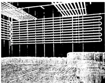
8.07 Air coolers are designed with the refrigerant flowing inside tubes or channels and the air passing on the outside. As the heat transfer coefficients during evaporation of the refrigerant are at least ten times those on the air side, at moderate air velocities, the outside surface area is usually increased by the use of fins. However, bare tubes are still used in older large ammonia systems. Figure 8.07 shows the interior of a cold store with bare tube evaporators. In this case, heat is transferred on the air side by free or natural convection, i.e. no fans are used to increase the air velocity across the tubes.
8.08 In most small systems as well as in modern large systems finned coil evaporators (cooling batteries, plate-fin-tube evaporators) are used. These consist of one coil, or several coils in parallel, attached to plate fins, in a housing. A fan is connected to force the air through the battery (Figure 8.08). This type of evaporators are manufactured in every size from one kW or less to hundreds of kW. The tubes are usually made of copper (aluminum or steel for ammonia), and the fins of aluminum. The fins are attached by expanding the copper tubes after the assembly of the unit. Good contact between the fin and the tube is of great importance for the heat transfer performance. Usually, the fin is shaped into a collar around the tubes. This collar then also acts as a spacer during production to get the right fin distance.
The fin spacing varies considerably depending on the application. For non-frosting conditions in small systems fin spacings down to 2 mm may be found. For large systems below 0°C spacings up to 12 mm are used.
The fin thickness is usually in the range 0.1 to 0.5 mm. The thickness is often chosen to achieve a certain stability of the fin rather than from heat transfer concerns.
The coil depths range from 40 to 500 mm. Coils with depths <200 mm are preferred, except in cases where the fin spacing is very large. With standard tube spacing this corresponds to a maximum of six tube rows.
8.09 In certain applications, e.g. where high air velocities cannot be tolerated, finned evaporator coils with free convection are being used. A typical design is shown in Figure 8.09a. With free convection, the fin spacing has to be larger than in forced convection, typically 10-15 mm.
Figure 8.07.: Interior of cold store with bare tube evaporators.
Another type of free convection evaporator is used in most domestic refrigerators. It is called
roll-bond evaporator (Figure 8.09b) and consists of two plates which have been bonded together over almost their entire surface. The area which is not bonded forms the evaporator channel. After the bonding procedure, which is done in a rolling process, the channels are inflated by high pressure. The expansion device (orifice) is often incorporated in the evaporator simply as a narrow section in the channel.
8.10 If the evaporator surface temperature is below the dew point of the air, the humidity will fall out as water or frost on the surface. As the water deposits on the surface, the heat of vaporization (and for frost, the heat of melting) is transferred to the surface together with the
sensible heat of the air. This latent heat transport must be considered when calculating the capacity of the evaporator.
Figure 8.09b.: Roll-bond evaporator.
At evaporation temperatures below 0°C it is necessary to arrange defrosting at regular intervals. If the room temperature is above 0°C defrosting may be arranged simply by turning off the compressor. More frequently, however, some active way of defrosting is arranged. This can be done either by electric heaters mounted in parallel with the evaporator tubes in the plate fins, or by reversing the refrigerant flow. In the second case, a reversing valve is installed as shown in Figure 8.10. During defrosting, the evaporator acts as condenser and the condenser as evaporator. This is called hot gas defrosting.
As heat is given off to the surrounding during defrost it is important that it is done as quickly as possible. With electric heaters, the power should be at least three times the capacity of the evaporator. With forced convection evaporators, the fan should be turned off during defrost (except at room temperatures >0°C and when defrosting is accomplished by the room air). The defrosting can be initiated at regular time intervals or ”on demand”. Several types of sensors can be used to detect the frost and initiate defrosting: In forced convection evaporators, the air pressure drop or the fan power can be used as frost indicators. In both forced and free convection systems it is possible to measure the difference between the evaporation temperature and the air temperature. With frost forming on the surfaces this difference will increase. Photocells, infra-red detectors and electric conductivity-sensors have also been used as frost detectors.
The defrosting is usually aborted by a defrosting thermostat mounted in between the fins of the evaporator, terminating the defrosting when the temperature has increased above 0°C. Alternatively, defrosting may be terminated simply after a pre-set time period.
The water formed during defrost is collected on a defrost pan below the evaporator and led through a tube to a drain outside the freezing room. Both the defrost pan and the tube must have electric heating to keep the water from freezing.
More information about frosting and defrosting of evaporators is given in Chapter 15 (partII)
Liquid Coolers
8.11 Liquid coolers are primarily used for cooling of brine in indirect systems, i.e. in systems where the cooling capacity is distributed by water with anti-freeze additives. They are also used for cooling of other liquids in industrial applications.
Figure 8.11 shows two different types of shell and tube evaporators. In the first, the refrigerant flows inside the tubes, while in the second, the brine flows in the tubes.
With refrigerant inside the tubes, the refrigerant may be evaporated completely (dry expansion). Notice the baffle plates which force the brine to flow up and down across the evaporator tubes, increasing the flow velocity, and thereby the heat transfer coefficient. The
baffles also result in a more ordered temperature distribution in the brine. This is a common type of liquid cooler for both small and large systems. Evaporation inside tubes has some advantages compared to outside evaporation: First, there is no risk of oil accumulating in the evaporator as the flowing refrigerant will transport the oil to the evaporator exit, second, the refrigerant charge will be much smaller.
An advantage of shell-side evaporation on the other hand is that the brine/liquid side is more easily accessible for cleaning. This is important for example in heat pump systems recovering heat from sewage water.
With shell side evaporation, the oil return problem is identical to that in other types of flooded evaporators as discussed above.
8.12 For smaller systems, coaxial evaporators have been widely used. This type of evaporator consists of two coaxial tubes, usually wound up as shown in Figure 8.12. The refrigerant runs in the inner tube. This tube may be smooth or have some type of surface structure to increase the surface area on either of, or both, the inner and outer surface.
Coaxial evaporators are intended for dry expansion.
Figure 8.11a.: Shell and tube evaporator with refrigerant inside tubes.
8.13 Since their introduction, brazed plate heat exchangers have steadily gained in popularity as evaporators for small systems (Figure 8.13). This type has to a large extent ousted the coaxial evaporators from the market. The plate heat exchangers are extremely compact, and therefore also have a small internal volume. This is important as it results in low refrigerant charges. This type of evaporator is generally recognized to give high overall heat transfer coefficients. The available sizes of brazed plate heat exchangers are steadily increasing and they are now manufactured for cooling capacities above 400 kW.
As copper is normally used for the brazing, brazed plate heat exchangers cannot be used for ammonia. Instead, semi-welded plate heat exchangers are used. In these, pairs of plates are welded together forming the refrigerant flow path. The welded pairs are stacked in a frame, held by bolts, with gaskets in between each pair. This type of evaporators is manufactured for cooling capacities up to 5000 kW and more.
8.14 Another type of plate evaporator is used in large heat pumps when heat is extracted from lake- sea- or sewage water. In this type, the refrigerant is enclosed between two vertical steel
Figure 8.12.: Coaxial evaporator
Figure 8.13.: Brazed plate heat exchanger, semi-welded plate heat exchanger
plates, and water is allowed to flow across the outside of the plates (Figure 8.14). With this design, the evaporator is easy to clean and there is no risk of damage due to freezing. Low temperature water can therefore be used as a heat source, and the water can be cooled to temperatures close to 0°C.
Solid heat source evaporators
8.15 As already mentioned, solid heat source evaporators are used only in special applications such as freezers in the food industry and heat pumps using the bedrock or soil as heat source. In general, the heat transfer is extremely good between the evaporator and the solid heat source. The heat transfer rate is in this case determined by the thermal conductivity of the solid material.
A contact plate freezer for packaged foodstuff is shown in Figure 8.15. The packages, containing e.g. fish fillets or chopped vegetables, are placed in-between horizontal evaporator plates. The good thermal contact ensures quick freezing of the product.
Ground source heat pump evaporators usually consist of a plain copper tube buried in the ground or inserted into a water-filled hole in the bedrock. When the soil is used as heat source, it is primarily the latent heat released as the water in the soil freezes which is extracted. The water content in the soil thus has a large influence on the necessary tube length.
C. Heat transfer
Introduction8.16 As an introduction to heat transfer we will return to the Figure of the temperature profile in the evaporator (Figure 8.16). Here, the temperature profile is slightly idealized as the influence of friction pressure drop and superheat of the refrigerant at the evaporator exit are neglected. Also, we are considering a pure fluid, not a refrigerant mixture.
If we study only a small part of the evaporator we may consider the temperature difference between the fluids as constant and the heat flow across the small area As is then calculated as
ϑ ⋅ ⋅ = s s U A Q& 8.16a
When considering the whole evaporator we have to take into account that the temperature difference changes from one end of the evaporator to the other. The cooling capacity of the evaporator is then calculated as
&
Q= ⋅ ⋅U A ϑm 8.16b
where Q = & cooling capacity (W)
U = overall heat transfer coefficient (W/(m2 K))
ϑm= mean temperature difference between the fluids (K)
With the idealization mentioned above, and assuming that the overall heat transfer coefficient is constant along the evaporator, it can be shown that the mean temperature difference ϑm should
be calculated as the logarithmic mean of the inlet and outlet temperature differences.
Figure 8.16.: Temperature profile in evaporator
Inlet temperature difference, ϑi evaporation temperature Refrigerant Temp Area Heat source Outlet temperature difference, ϑo
ϑ ϑ ϑ ϑ ϑ m i o i o = − ln 8.16c
Eq. 8.16b can be used to calculate the capacity of an evaporator with a known surface area, or to calculate the area necessary to achieve a certain capacity. In either case the overall heat transfer coefficient and the mean temperature difference must be known. The overall heat transfer coefficient is primarily a function of the surface heat transfer coefficients on the refrigerant side and on the heat source side, and most of the remainder of this chapter will be devoted to the calculation of these heat transfer coefficients.
The mean temperature difference, however, can be chosen arbitrarily as long as Q& and A are not both fixed. The choice of the temperature difference is a matter of economic optimization rather than technical: If a small temperature difference is selected, a large (expensive) surface area is necessary - if the temperature difference is large, a small area will be sufficient, but the
COP of the plant will be low, resulting in high running costs. In the last part of the chapter some guidelines for economical optimum temperature differences will be given.
8.17 Example - Mean temperature difference
A cooling battery is installed in a cold room. The room temperature is +6°C and the air temperature is reduced by 6°C as it passes through the battery. Calculate the logarithmic mean temperature difference if the evaporation temperature is -2°C.
Solution:
The temperature differences at the inlet and outlet are, respectively:
ϑi = +6 - (-2) = 8 K
ϑo = 0 - (-2) = 2 K
According to eq. 8.16b the logarithmic mean temperature difference is then
K 33 . 4 2 8 ln 2 8 ln = − = − = o i o i m ϑ ϑ ϑ ϑ ϑ
8.18 The overall heat transfer coefficient is defined by the equation 8.16a. Note that the surface areas usually are different on the refrigerant side and on the heat source side and that the overall heat transfer coefficient will be different depending on which area it is referred to. Because of this, it is convenient to speak of the evaporator’s U⋅A-value instead of the overall heat transfer coefficient.
8.19 The heat transfer on either side of the heat transfer wall is calculated by Newton’s law of cooling, which is also the defining equation for the (film) heat transfer coefficient α:
&
Q = α⋅A⋅ϑ 8.19a
The heat transfer by conduction through the heat transfer wall is determined by Fourier’s law, which is the defining equation for the thermal conductivity
&
Q A t
x
= − ⋅ ⋅λ δ
∂ 8.19b
For a plane surface at steady state (Q , & λand A all constant) this simplifies to
&
Q= ⋅ ⋅λ A
δ ϑ 8.19c
where δ is the thickness of the wall andϑ is the temperature difference between the inside and outside surfaces (the minus sign is now incorporated in ϑ).
8.20 It is often convenient to speak of thermal resistances rather than heat transfer coefficients and thermal conductivities. These resistances are analogous to electric resistances in electric circuits and are defined by the thermal counterpart to Ohm’s law for electric circuits
Ohm’s law: Electric resistance = Electric potential / Current
The thermal resistanceR is thus defined as
R = ϑ / Q & 8.20a
Comparing this to equation 8.16a we find that the total thermal resistanceRt isthe inverse of the U⋅A-value
Rm = ϑm / Q = & 1 / (U⋅A) 8.20b
Likewise, we may define the thermal resistances between any of the two fluids and the heat transfer wall as
Rf = 1 / (α⋅Af) 8.20c
and the resistance in the heat transfer wall as
Rw = δ /(λ⋅Aw) 8.20d
where Aw is some mean of the outside and inside surface areas. (For a cylindrical wall Aw is the logarithmic mean, for a sphere it is the geometric mean).
8.21 As the heat flow is constant in the flow direction, we have
&
This relation can be used to express the temperature differences (e.g. ϑm = Q&/(U⋅A)).
But the temperature differences are related by
ϑm = ϑ1 + ϑw + ϑ2 8.21b
By inserting the expressions for the temperature differences we find that
1 1 1 1 1 2 2 U A⋅ =α ⋅A + ⋅ + ⋅Aw A δ λ α 8.21c or Rm = R1 + Rw + R2 8.21d
The total thermal resistance is thus the sum of the thermal resistances in the two fluids and in the intermediate wall, and the overall heat transfer coefficient is a function of the film heat transfer coefficients in the two fluids, of the surface areas and of the thickness and conductivity of the wall.
Figure 8.21 shows schematically the temperatures and the temperature differences for a section of a smooth tube evaporator.
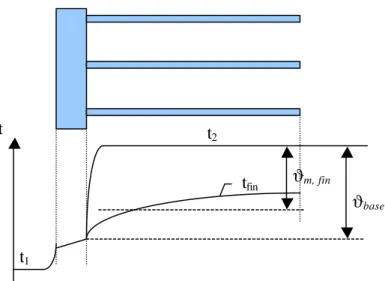
8.22 For finned surfaces, the surface temperature of the fin will increase towards the tip of the fin as is shown in Figure 8.22. Because of the lower temperature difference between surface and fluid, the heat flux due to convection will be lower on the fin than on the base surface in between fins. The fin surface is thus less efficient than the base surface, and a fin efficiencyξf
is defined as the ratio between the actual heat transferred and the heat which would be transferred if the whole fin had the temperature of the fin base. Assuming equal heat transfer coefficients on the fin and on the base, this ratio is equal to the ratio between the mean fin temperature difference, ϑm, fin, and the base temperature difference, ϑbase (see Figure
8.22a).
Figure 8.21.: Local temperature profile for smooth tube evaporator. ϑw t t2 ϑ2 ϑm ϑ1 t1
base fin m base fin m idealfin actual f A A Q Q ϑ ϑ ϑ α ϑ α ξ , = , ⋅ ⋅ ⋅ ⋅ =
≡ && 8.22a
For a straight fin with constant cross section, it may be shown that the fin efficiency may be calculated as ξf m L m L = tanh(⋅ ⋅ ) ( ) 8.22b
where L = the length of the fin (m)
m P
A
=αλ⋅⋅
1 2/
8.22c where α = heat transfer coefficient (W/(m2 K))
P = perimeter of the fin (m)
A = cross section area of the fin (m2)
λ = thermal conductivity of the fin (W/(m K))
For other types of fins, the fin efficiency may be estimated from the diagram in Figure 8.22b. When determining the overall heat transfer coefficient, or the total thermal resistance, for a finned surface, the area for the finned side is calculated as
Atot = Abase + ξf ⋅ Afin 8.22d
and the overall heat transfer coefficient from:
Figure 8.22a.: Local temperature profile for finned surface.
tfin ϑm, fin
t t2
ϑbase
1 1 1
1 1 2
U A⋅ =α ⋅A + ⋅Aw + ⋅ Abase + ⋅f Afin δ
λ α ( ξ ) 8.22e
where A1 = inside surface area (m2)
Abase = outside surface area in between fins (m2)
Aw = logarithmic mean of in and outside surface areas of tube (m2)
Afin = fin area (m2)
8.23 Before going into the details of calculating the surface heat transfer coefficients, approximate values of overall heat transfer coefficients for different types of evaporators are presented in Table 8.23a. The values are referred to the logarithmic mean temperature difference and to the total surface area on the heat source side.
In Table 8.23b approximate values for film heat transfer coefficients are presented. For cases where the heat transfer areas are known, this table can be used for estimating the overall heat transfer coefficient. Also, by comparing the two tables, the dominating thermal resistance
Table 8.23a, Approximate U-values for different types of evaporators. (Based on Pierre, 1979).
Type of evaporator Fig. no U W/(m2 K)
Notes Air coolers
Free convection
Smooth tubes 8.07 9-13 Depending on temp. difference, tube diameter and position
Plates 8.09 12-14 Below 0°C, ≤ 12 W/(m2 K)
Finned coils 8.09 4-8 Depending on temperature difference, fin distance, number of tube rows, position
Forced convection
Smooth tubes 30-60 Air velocity 3-5 m/s Tube diameter 25-50 mm Finned coils 8.08 12-25 Air velocity 2-4 m/s
Heat flux at inner surface 2000-5000 W/(m2). Dry expansion.
Liquid coolers Free convection
Smooth tubes in brine tank, refrigerant inside tubes
100-170 Brine temp. -30-0°C
U reduced by 20% in dry expansion Smooth tubes in brine tank,
brine inside tubes
120-170 Brine temp. -30-0°C
Brine velocity inside tubes 1.5 m/s Smooth tubes in water tank,
brine inside tubes
180-220 Brine velocity 0.5 - 1.5 m/s Brine temp. -8 - 0°C Forced convection
Shell and tube, brine inside tubes, NH3 as refrigerant
8.11a 200-500 Brine velocity 0.5 - 1.5 m/s Shell and tube, brine inside
tubes, (HC)FC as refrigerant
8.11a 150-400 Brine velocity 0.5 - 1.5 m/s Shell and tube, (HCFC)-
refrigerant inside tubes
8.11b 250-600 Brazed plate heat exchanger,
(HC)FC as refrigerant
Table 8.23b.: Approximate film heat transfer coefficients (Based on Ekroth/Granryd, 1994)
Type of flow Approximate heat transfer
coefficient (W/(m2⋅°C)) Turbulent flow in tubes,
(diameter ≈ 50 - 25 mm)
Water (0.5 - 5 m/s) 1500 - 20000
Air (1 - 10 m/s) 10 - 50
Laminar flow in tubes, (diameter ≈ 50 - 10 mm)
Water 50 - 250
Air 2 - 15
Air flow past plates (1 - 10 m/s) 10 - 50 Natural convection Water 200 - 1000 Air 2 - 10 Condensation Water 5000 - 15000 Refrigerants 1000 - 5000 Boiling Water 1000 - 40000 Refrigerants 200 - 5000
Heat transfer in boiling
8.24 The physical mechanisms of boiling processes are extremely complicated and cannot be modeled in any detail. The correlations used for calculating heat transfer coefficients in boiling are therefore empirical or semi-empirical.
8.25 Boiling of a stagnant pool of liquid (no forced convection of the liquid) is referred to as pool boiling. Depending on the heat flux different types of pool boiling may appear (c.f. Figure 8.25). At low heat fluxes, heat is transferred from the heated surface to the liquid without bubble formation. The liquid close to the heated surface is slightly superheated, and the heat is transferred through the liquid by free convection to the liquid surface (which has saturation temperature) where evaporation takes place. As there is no bubble formation at the heated surface this is usually not referred to as boiling but as free convection evaporation or
surface evaporation. Heat transfer in this region can be calculated by correlations for free convection.
At higher heat flux, bubble formation will start (point A in Figure 8.25), resulting in higher heat transfer coefficients. This is the nucleate boiling region and it is by far the most important region for technical applications. The high heat transfer coefficients can be attributed to vigorous convection in the liquid in conjunction to the bubble formation, and to the bubble formation itself. As the heat flux is increased, the amount of bubbles at the surface will increase steadily, and eventually the bubbles will form a vapor layer insulating the surface from the surrounding liquid (point C in Figure 8.25). Increasing the heat flux above this critical value will result in drastically reduced heat transfer coefficients, which in turn will lead to a sudden increase in the temperature difference (to point D). As the temperature at this point may well be above the melting point of the heated surface, point C is referred to as the burnout point
and the corresponding heat flux as the critical heat flux. For the boiling in refrigeration
evaporators, however, the heat fluxes are far below this point.
8.26 Free convection heat transfer can generally be expressed in dimensionless form as
Nu = C ⋅ (Gr ⋅ Pr)n 8.26a
where Nu = α⋅H/λ Nusselt no
Gr = g⋅β⋅ϑ⋅H3 / ν2 Grashof no Pr = µ⋅cp / λ Prandtl no
This expression is also valid for the free convection evaporation region. The constant C and the exponent n depend on the geometry and on the product (Gr⋅Pr) and are given for a few cases in table 8.26. The characteristic length used in the Grashof no is the height for vertical plates or cylinders, and the diameter for horizontal tubes.
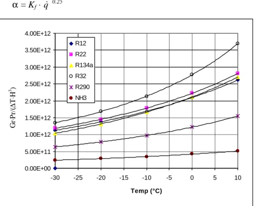
The factors (Gr⋅Pr/(ϑ⋅H3)) for some pure refrigerants are shown in Figure 8.26 as a function of temperature.
In the turbulent region (i.e. when Gr⋅Pr > 109) the heat transfer coefficient is independent of the characteristic length and the above equation leads to the expression
α = Kf ⋅q& 0.25 8.26b
Table 8.26, adapted from Holman, 1992
Geometry Gr⋅Pr C n
Horizontal cylinders 104 - 109 0.53 0.25
109 - 1012 0.13 0.33
Vertical planes and cylinders 104 - 109 0.59 0.25 109 - 1013 0.10 0.33 0.00E+00 5.00E+11 1.00E+12 1.50E+12 2.00E+12 2.50E+12 3.00E+12 3.50E+12 4.00E+12 -30 -25 -20 -15 -10 -5 0 5 10 Temp (°C) GrPr/(DtH3) R12 R22 R134a R32 R290 NH3
Figure 8.26.: The factor Gr⋅Pr/(ϑ⋅H3) for a few pure refrigerants
Gr ⋅ Pr/( ∆ T ⋅ H 3 )
where q&= Q A &/ = surface heat flux (W/m2)
and Kf = constant
Through the relation q& = α ⋅ϑ we may also express the temperature difference as
ϑ = q& 0.75 / Kf 8.26c
The values of Kf are different for each refrigerant, but are fairly independent of temperature. Table 8.26b shows the values for horizontal tubes for a few pure refrigerants at -10°C. For
vertical plates or cylinders the values should be multiplied by 0.82.
8.27 For the nucleate boiling region, several correlations for the heat transfer coefficient are found in the literature. A common characteristic of these are that
α ∝ q& m where 0.6 < m < 0.8
This relation is valid also for some types of flow boiling. Another common characteristic is that the heat transfer coefficient increases with increasing pressure.
When different correlations are compared, it is found that the results may differ considerably, often by 30% or more. The reader is therefore advised not to expect too high accuracy in the estimation of pool boiling coefficients.
The following simple correlation which is considered to be fairly accurate was proposed by Cooper (1984).
αpb = C ⋅ 55 ⋅pr(0.12-0.2 ⋅ log Rp)⋅ (-log pr) -0.55⋅ M -0.5⋅q& 0.67 8.27a
where pr = reduced pressure (= p / pcrit)
Rp = surface roughness (µm)
M = molecular weight
The value of the constant C is 1 for horizontal, plane surfaces and 1.7 for horizontal copper tubes, according to Cooper’s original paper. However, comparisons with experimental data suggests that better agreement is achieved if a value of 1 is used also for horizontal tubes. Note that the heat transfer coefficient is a fairly weak function of the surface roughness parameter Rp, which is seldom well known. A value of Rp = 1 is suggested for technically smooth surfaces. The correlation may thus be expressed in the simple form
αnb = Knb ⋅q& 0.67 8.27b
where Knb is a function of the reduced pressure and the molecular weight of the refrigerant.
Table 8.26b: Values of constant Kf in equations 8.26 b and c
Kf R12 R22 R134a R32 R290 NH3
8.28 The above relation is valid for single smooth tubes and smooth horizontal surfaces. For tube bundles the average heat transfer coefficient will be slightly higher as the heat transfer is enhanced by the convection caused by the rising bubbles. This can be taken into account by multiplying the heat transfer coefficient for the single tube by a bundle factor. For plain and low finned tubes this factor typically is about 1.5.
A better estimate my be found by using a method proposed by Gorenflo (1993). According to this method, a mean heat transfer coefficient for the bundle is calculated as
αmean = (αnb,one + f ⋅αf) [ 1+ (2 + q&)-1] 8.28
where αnb,one = heat transfer coefficient for single tube in nucleate boiling f = factor depending on bundle size and inlet velocity (0.5 < f < 1)
αf = free convection heat transfer coefficient (according to 8.26)
&
q = heat flux in kW
8.29 Pool boiling evaporators are often made of finned tubes. If the surface heat flux and the heat transfer coefficients both are referred to the total surface area, the boiling heat transfer coefficients of the finned tubes are slightly higher than for smooth tubes. The increase can be attributed to good contact between the surface and the bubbles as these rise in between the fins.
8.30 Flow boiling inside tubes or channels is considerably more complex than pool boiling. As part of the liquid is evaporated, the volume of the refrigerant is increased greatly, causing an
2.00 3.00 4.00 5.00 6.00 7.00 8.00 9.00 -30 -25 -20 -15 -10 -5 0 5 10 Temp (°C) K R12 R22 R134a R32 R290 NH3
Figure 8.27.: Pool boiling constant of equation 8.27b for some refrigerants.
Evaporation temp (°C) Knb ((W/m 2 ) 0.33 /K)
acceleration of the fluid. Investigations of flow boiling have shown that the process may be divided into different flow regimes (Figures 8.30a and 8.30b). The mechanisms of heat transfer are different from one regime to another. Two main heat transfer mechanisms may be discerned: nucleate boiling and convective boiling. In convective boiling, nucleation is suppressed and evaporation takes place at the liquid/vapor interface. To calculate the heat transfer at each point along an evaporator tube it would be necessary to know where one flow regime ends and another starts. A number of investigators have studied the flow regimes in two phase flow, and their dependence on different parameters. The results are usually presented as flow-regime maps where the regime is shown as a function of e.g. mass flux and vapor quality. Studies of the flow in vertical and horizontal tubes have shown that the flow regimes are basically independent of the orientation of the tube. Only at low heat- or mass fluxes the flows are considerably different, as, in horizontal tubes, the gravitational forces will stratify the flow.
Figure 8.30a.: Flow regimes in horizontal flow
Stratification has a large influence on the heat transfer as the coefficient of heat transfer is very low between the vapor and the tube wall. The dry part of the tube in this case acts as an extended surface, transferring heat to the submerged portion of the tube wall.
It is generally said that when the vapor quality is less than 5-8% (Rohsenow and Hartnett 1973) the heat transfer mechanism is closely related to that in pool boiling, the main difference being that in forced convection boiling there is a velocity parallel to the heated surface. In evaporators of heat pumps and refrigeration equipment however, the heat flux is often too small to initiate nucleate boiling even in the low quality region. In vertical evaporators, like plate heat exchangers, the heat transfer coefficient at low heat fluxes are found to be reasonably well predicted by pool boiling correlations.
At higher vapor qualities, the acceleration of the vapor-liquid mixture causes an annular flow, with vapor traveling at high speed in the center of the tube, and liquid covering the walls. In some cases the vapor contains a large amount of liquid drops. In annular flow, heat is transferred by convection through the liquid film and the evaporation takes place at the liquid-vapor interface. At low heat- or mass fluxes, annular flow may never be reached, and the flow may be more or less stratified along the whole evaporator.
Finally, at a vapor quality somewhere between 70 and 100%, the liquid film dries out and only liquid droplets, dispersed in the vapor flow, remain to be evaporated. This kind of flow is called mist flow or dispersed flow. Here, heat is transferred partly by convection through the superheated vapor to the liquid drops, but also by the drops hitting the walls and evaporating on contact.
Figures 8.30a and b indicate that other regimes than the three discussed above may be present in the tube, but often three flow regimes are considered enough to describe boiling heat transfer inside a tube.
8.31 As stated above, different heat transfer mechanisms are dominant in the different flow regimes, and for an accurate calculation of the heat transfer coefficients along an evaporator tube it would be necessary, first, to have an accurate correlation for predicting the flow regimes and, second, to have accurate correlations for the heat transfer coefficient in each regime. As of today there are no such correlations available, and the heat transfer is estimated by simplified empirical or semi-empirical correlations.
100 1000 10000 100 1000 10000 100000 q (W/m2) alfa (W/(m2 K)) 50 kg/(m2/s) 100 kg/(m2/s) 150 kg/(m2/s) 200 kg/(m2/s) 250 kg/(m2/s) Convective evaporation Nucleate boiling
Figure 8.31a.: Schematic diagram of heat transfer coefficient in flow boiling as a function of heat flux and mass flux.
In many cases in traditional refrigeration applications the heat transfer coefficient does not vary very much along the evaporator. It is then possible to use correlations for the mean heat transfer coefficient for the whole evaporator. Such correlations also have the benefit of being very simple to use compared to correlations for the local heat transfer coefficient.
In some more general correlations the local heat transfer coefficient is considered to be the net effect of the two mechanisms, nucleate boiling and convective evaporation. Some general observations can be stated concerning the heat transfer in these two regimes:
When nucleate boiling is dominant, heat transfer is strongly dependent of heat flux (α ∝ q&0.7) but only weakly dependent on mass flux and vapor fraction.
In the convective evaporation regime, the heat transfer coefficient is almost independent of heat flux, but increases with increasing mass flux and increasing vapor fraction. These general conclusions are shown schematically in Figures 8.31a and b. In both regimes, the heat transfer coefficient increases with increasing pressure.
8.32 One of the most well known correlations for the mean heat transfer coefficients was proposed by Pierre (1953). His original work was based on the boiling of R12 in horizontal copper tubes, heated by flowing water in a concentric tube. Later, the correlation was confirmed by Pierre (1957 and 1969) for R22 and R502 by further experiments and for R11 and methyl chloride by using experimental results of other investigators. Pierre (1969) gives two correlations, one for complete evaporation (5 - 7 K superheat) and one for incomplete evaporation:
Complete evaporation: Num = 1.0⋅10-2⋅(Re2⋅ Kf )0.4 8.32a
Incomplete evaporation: Num = 1.1⋅10-3⋅Re ⋅ Kf0.5 8.32b
where Num = αmean⋅d /λ mean Nusselt number
) /(
4
Re = ⋅m& π⋅d⋅µ Reynolds number
0 100 200 300 400 500 600 700 800 900 1000 0 0.2 0.4 0.6 0.8 1 Vapor fraction
heat transfer coefficient
F igure 8.31b.: Heat transfer coefficient as a sum of convective- and nucleate boiling contributions.
Total
Convective evaporation Nucleate boiling
Kf = ∆h / (L ⋅ g) Pierre boiling number ∆h = change in enthalpy between inlet and outlet (J/kg)
L = tube length (m)
g = acceleration due to gravity Conditions: Re2⋅ Kf < 3.5 ⋅ 1011
Num < 420
Since the article was published, more accurate data on the thermal conductivity and viscosity of refrigerants has been presented. The change in property data will directly influence the constants in the two equations and it is therefore suggested that the constants are reduced by 15%, if recent data for conductivity and viscosity is used.
Experimental results have shown that the Pierre equations give accurate results also with modern (HC)FC refrigerants (except R32). However, the predictions are according to some sources less accurate for hydrocarbon refrigerants (Melin, 1996).
8.33 One of several equations for the local heat transfer coefficient in which the heat transfer is assumed to be the sum of a nucleate boiling and a convective contributionwas suggested by
Gungor and Winterton (1986):
αtp = αnuc + αconv 8.33a
The nucleate boiling contribution αnuc is calculated from the pool boiling correlation of Cooper
(eq. 8.27a). However, as the nucleate boiling may be suppressed by the convection, they included a suppression factor, S, such that
αnuc = αpb ⋅ S 8.33b
The convective contribution they assumed could be described by a modified form of the Dittus-Boelter equation for one phase liquid flow (c.f. eq. 8.62a), multiplied by an
enhancement factorE, as the heat is transferred in this case through a thin liquid film which is disturbed at the surface by the evaporation:
αconv =αliq ⋅ E 8.33c
where
αliq = (kl/d) ⋅ 0.023 ⋅Rel0.8⋅ Prl0.4 8.33d
and
kl = liquid thermal conductivity (W/(m K))
Rel = G ⋅ d ⋅(1-x)/µl 8.33e
G = mass flux (kg/(m2 s)) x = vapor fraction
The enhancement factor is calculated as
E = 1 + 24000 · Bo1.16 + 1.37 ⋅ (1/Xtt)0.86 8.33f
where Bo = q&/(G⋅r) 8.33g
Xtt ≅ ((1-x)/x)0.9⋅ (ρv / ρl)0.5⋅ (µl / µv)0.1 8.33h
The suppression factor was found to be a function of the enhancement factor
S = (1+1.15⋅10-6⋅ E2⋅ Rel1.17)-1 8.33i
For horizontal tubes and Froude numbers FrL =G2/(ρ2⋅g⋅d) < 0.05 the enhancement- and suppression factors should be modified as follows:
Emod = E ⋅ FrL(0.1-2 ⋅ FrL) 8.33j
Smod =S ⋅ (FrL)1/2 8.33k
The correlation gives local heat transfer coefficients (circumferential averages for each point along the evaporator tube). When using this type of correlation it is necessary to divide the evaporator tube into five to ten sections, calculate a local value in the middle of each section and consider this as an average for the section.
8.34 For most types of evaporators the correlations presented above can be used directly. For
plate heat exchangers, however, the refrigerant flow channel is neither a liquid pool nor a circular tube. As of today there are no correlations suggested in the open literature for this type of heat exchanger. The designer is therefore more or less in the hands of the manufacturers who usually supply computer programs for choosing the correct size of heat exchanger. Test results published in the literature suggest that the heat transfer coefficients of plate heat exchangers is the sum of a nucleate boiling contribution and a convective contribution just as is the case for boiling in tubes. Some test data has been well correlated just using Cooper’s correlation for pool boiling (eq. 8.27a).
8.35 So far, we have assumed that the refrigerant is a pure substance and thus evaporates at constant temperature along the evaporator. For most refrigerant mixtures, however, this is not true and this has a considerable influence on heat transfer.
Refrigerant mixtures were discussed in some detail in Chapter 5, and the reader is assumed to be familiar with the terminology introduced there. In the following section we will concentrate on the implications on heat transfer of using mixtures.
When a zeotropic mixture boils the vapor formed has a higher concentration of the most volatile component than the boiling liquid. The composition of the liquid will therefore shift during evaporation towards higher concentration of the less volatile component and, because of this shift, the boiling point will increase. The difference in temperature between that at which boiling starts (the bubble point) and that at which all liquid is evaporated (the dew point) is called the glide of the mixture. The glide is a function of the components, the concentration of the components and of the pressure. For some zeotropic mixtures the glide is small and has therefore little influence on the system. These are referred to as near-azeotropes. There is no strict definition of how large the glide can be of a near-azeotrope, but a glide of a couple of degrees will have a noticeable influence on heat transfer and on the system.
8.36 If a zeotropic refrigerant is used in a pool boiling or re-circulation type evaporator, the concentration of the less volatile component will be higher than in the original charge in the liquid in the evaporator and lower in the circulating refrigerant. This leads to an increase in the condensing pressure and a reduction in the evaporation pressure, which in turn leads to a decrease in the capacity of the system.
The heat transfer coefficient in the evaporator will be lower than the weighted average of that of the pure components. The main reason for this is that as the liquid boils, the more volatile component is concentrated in the bubbles and transferred to the liquid surface, while the less volatile component is concentrated close to the heated wall. This leads to an increase in the bubble point at the wall and therefore also to an increase in the temperature difference between the wall and the liquid bulk (Figure 8.36).
If the heat transfer coefficient is defined as for a pure fluid
α = q& / (twall - tbubble) 8.36
where tbubble is now the bubble point of the liquid bulk it is evident that the extra temperature
difference associated with the difference in concentration will seem to decrease the heat transfer coefficient.
A second reason for the decrease in heat transfer is that the thermodynamic properties (conductivity and viscosity) of a mixture are usually less favorable to heat transfer than the weighted average of the properties of the pure components. Also, it has been shown that the nucleation of bubbles is impaired, leading to fewer active nucleation sites.
The increased concentration of the less volatile component in the evaporator and of the most volatile component in the circulating refrigerant will also cause other problems in the system. Because of the low heat transfer and these other problems it is recommended not to use pool boiling or re-circulation-type evaporators with zeotropic mixtures.
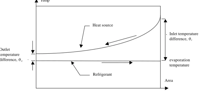
8.37 In dry-expansion evaporators zeotropic mixtures are more easy to handle, and may even have some benefits. Because of the glide, the refrigerant temperature will increase along the
Figure 8.36: Temperature profile in boiling refrigerant mixture near heated wall.
twall
tbubble, wall
evaporator with increasing vapor fraction. If this increase is matched with the temperature decrease of the heat source fluid (in counter-current flow) it can be shown that the thermodynamic efficiency (COP) can be higher for a mixture than for a pure fluid.
In Figure 8.37 the temperature profiles of a mixture and of a pure fluid are shown. The mass flow of the heat source fluid is assumed to be the same, and as the temperature change of this fluid is also the same in both cases, the cooling load Q& is equal. Assuming also that the overall heat transfer coefficients are equal for the mixture and the pure fluid, and remembering that
&
Q = U ⋅ A ⋅ϑm 8.37
we find that the logarithmic mean temperature differences must also be equal.
However, from the figure it is clear that the evaporation temperature will be higher with the mixture than with the pure fluid. As the COP of a refrigeration cycle is approximately inversely proportional to the temperature difference between the evaporator and the condenser, it is clear that the mixture should be expected to give higher COPs under the assumptions stated above. Note that this gain can only be achieved with counter-current flow!
8.38 In practice, the overall heat transfer coefficient cannot be expected to be the same for the mixture and the pure fluid as the boiling heat transfer coefficient will be lower for the mixture. The reasons for the decrease in the heat transfer coefficient are basically the same as in pool boiling: Concentration of the least volatile component at the heated surface, less favorable thermodynamic properties and impeded bubble nucleation. The physical process is considerably more complex in flow boiling, however, for at least two reasons: First, there are concentration gradients not only perpendicular to the heated surface, but also in the axial direction of the tube and along the circumference. Second, as the vapor travels faster than the
Figure 8.37.: Temperature profiles in counter-current evaporator with a) mixture and b) pure fluid.
Evaporation temperature of pure fluid Temperature Area Temperature Area Pure fluid Mixture Mean evaporation temperature of mixture Equal areas
liquid inside the tube, the local conditions at any point will be in neither thermal (temperature) nor thermodynamic (concentration) equilibrium.
Several correlations have been suggested in the literature for calculating flow boiling heat transfer coefficients for refrigerant mixtures. Most of these are based on correlations for pure fluids. The correlations are often cumbersome to use and the accuracy is still in question. It is considered outside the scope of this text to suggest a correlation for flow boiling of mixtures. The interested reader is referred to Rohlin (1996), Melin (1996) or Steiner (1993).
8.39 A different problem which may hinder the possible benefits of glide-refrigerants is the necessity of superheat and the setting of the expansion valve. As shown in Figure 8.37 the temperature difference at the evaporator exit is considerably smaller with the mixture. For this reason, a larger part of the evaporator must be used for superheating.
To ensure stable operation of the expansion valve a superheat of 5-7 K is normally needed at the evaporator exit. With refrigerant- and heat source temperatures being parallel, this may be difficult to achieve, as the desirable mean temperature difference is usually of about this magnitude.
8.40 The pressure drop of evaporative two-phase flow inside a straight tube is the sum of three components: The wall friction pressure drop, the static pressure difference and the momentum pressure drop.
∆ptot = ∆pf +∆ps +∆pm 8.40
If the evaporator has bends, additional pressure drop is caused by these.
The wall friction pressure drop, ∆pf, is due to the shear forces between the flowing refrigerant and the tube walls, and to some extent between liquid and vapor. The static pressure difference, ∆ps, is caused by the gravitational force acting on the vapor/liquid column in the tube. The momentum pressure drop, ∆pm, is the effect of the increase in velocity (or kinetic energy) of the vapor/liquid mixture inside the tube.
8.41 The static pressure drop of a tube with height H is calculated as
∆ps =
∫
Hρmdz0 8.41a
The difficulty in this equation is to determine ρm, the density of the liquid/vapor mixture. If the
homogeneous model, in which the velocities of the two phases are considered to be the same, is applied, ρm may be calculated from:
1/ρm = vm =(1-x) ⋅ vl + x ⋅ vv 8.41b
where vl = specific volume of liquid
vv = specific volume of vapor
The integration of equation 8.41b may be avoided by dividing the evaporator into sections and assuming the density to be constant in each section. The vapor fraction can, for an estimate, be assumed to increase linearly along the evaporator and the density can thus be calculated for each section.
Alternatively, the mean density of the mixture can be calculated as proposed by Pierre (see Section 8.44).
8.42 The momentum pressure drop is a result of a velocity increase of the refrigerant. This increase may be due to a decrease in the tube diameter or to an increase in the specific volume. The specific volume will increase as the refrigerant evaporates due to either heat transfer or pressure drop.
The momentum pressure drop can be written in terms of the difference in kinetic energy of the mixtures entering and leaving the evaporator:
∆pm = G2⋅(vm2 - vm1)/2 8.42a
Where G is the mass flux in the tube (kg/(m2 s)) and vm2 and vm1 are the specific volumes of the mixtures leaving and entering the evaporator respectively.
If the liquid and the vapor are considered to be traveling at the same velocity (a condition of no slip), vm1 and vm2 may be calculated by eq 8.41b. In this case, the momentum pressure drop may also be written as
∆pm = (ρm2⋅w22)/2 - (ρm1⋅w12)/2 8.42b
where w1 and w2 are the velocities of the refrigerant entering and leaving the evaporator respectively. This clearly shows the relation to kinetic energy.
Note that a quick estimate of the upper bounds of the momentum pressure drop of a dry expansion evaporator is found by using the vapor and liquid specific volumes in equation 8.42b.
8.43 Most correlations for frictional pressure drop belong to either of two groups: The homogeneous models, where liquid and vapor are assumed to travel at the same velocity as a homogeneous mixture, and the separated flow models, where the phases are considered as separated flows, which may be flowing at different velocities.
In both type of models, the pressure drop of the two phase flow ∆ptp may be related to the
pressure drop of one phase flow ∆pl (as calculated by standard correlations) by a two phase
multiplier, φ2, defined by:
∆ptp / ∆pl = φ2 8.43a
where φ2 is a function of flow- and heat transfer parameters and of fluid properties. Only homogeneous models will be treated here. It should be noted that the accuracy in the prediction of any of the existing models is quite low.
In the homogeneous models, average properties are assigned to the liquid/vapor flow and existing single phase correlations are used to evaluate the pressure drop. The frictional pressure drop may then be written as
∆p f w ddz f m l =
∫
⋅ρ ⋅ 2⋅ 0 1 8.43bwhere ρm is calculated from equation 8.41b, and w = G / ρm, flow velocity
d = diameter of the tube
f = friction factor
The simplest, but less accurate method of determining f is to use the one-phase friction factor for turbulent flow from the Blasius equation
f = 0.158 Re-¼ 8.43c
or from Moody's diagram.
The Reynolds number in the above equations is determined as
Re = ⋅ = ⋅ & ⋅ ⋅ G d m d µ π µ 4 8.43d
where m& is the mass flow and µ is a mean viscosity which may be calculated as (McAdams, 1942) 1 1 µ = µ + µ − x x v l 8.43e
Instead of integrating equation 8.43b it is suggested (Griffith, 1973) that the evaporator is divided into a number of sections and the vapor quality assumed to be constant within each section.
8.44 Special friction factors for two phase flow have also been suggested. Pierre (1957) investigated the evaporation of R12 and R22 in horizontal tubes and concluded that the mean friction factor for oil free refrigerant can be expressed as (c.f. one-phase flow)
∆pf =fm⋅ G2⋅ vm ⋅ L/d 8.44a
if the friction factor is determined as
fm = 0.0185 ⋅ Kf1/4⋅ Re-1/4 8.44b
where Kf is the Pierre boiling number, Kf = ∆h /(L ⋅ g), and the Reynolds number is calculated
using the liquid viscosity.
In the presence of oil, (6-12%) a considerably higher friction factor was found
fm = 0.053 ⋅ Kf1/4⋅ Re-1/4 8.44c
vm = xm⋅vm” 8.44d
where xm is the mean vapor fraction, calculated as
xm = 4.4 ⋅d1/4⋅L-1/2 8.44e
and vm” is the specific volume of the vapor at average evaporation temperature. The correlation for xm was based on experimental results.
Note that no integration of equation 8.43b is necessary with this method.
Methods of enhancing boiling heat transfer
8.45 Heat transfer in pool boiling and in nucleate boiling in general may be enhanced, without increasing the surface area, by facilitating the nucleation of bubbles. The most commonly used method of achieving this is by giving the surface a rough or porous texture.
One of the first studies of the influence of surface finish on heat transfer was done by Jakob and Fritz (1931). They boiled water at atmospheric pressure on several specially prepared horizontal copper plates. Of these, one was sandblasted and one had a square grid of finely machined grooves. They found that sandblasting the surface increased the heat transfer coefficient by 25% at a given heat flux. The grooved surface increased the heat transfer coefficient even more, initially about 300%. Both increases diminished with time and the heat transfer coefficients tended towards those of a smooth surface.
The findings during the 1950’s that reentrant cavities (Figure 8.45a) functioned as stable nucleation sites stimulated the development of new evaporator surfaces. It was not until the 1970’s, however, that such surfaces became commercially available. A number of methods for manufacturing such enhanced surfaces, have been tried. Two groups of surfaces may be distinguished depending on the manufacturing method:
In the first group are found surfaces made by applying material to a smooth surface. They are usually made by flame spraying or sintering of metal onto the substrate to produce a porous layer.
The second group of surfaces are made by machining the surface of a smooth heat transfer wall (usually a low-finned tube) to form the desired reentrant cavity surface. Examples of geometries of commercial enhanced tubes are shown in Figure 8.45b.
The porous surfaces’ enhancement of heat transfer can be attributed to the following:
• During boiling in a porous structure, some vapor will be left when a bubble departs from the surface. This vapor will act as a ”mother-bubble” for new bubbles.
• In the porous structure the wetted surface area is very large.
• The boiling mechanism is evaporation of very thin liquid films, which can be expected to result in high heat transfer coefficients.
The heat transfer coefficients have been shown to increase by 100 to 1000% with these surfaces, compared to a smooth tube.
8:38
High Flux, (Union Carbide)
Thermoexcel-E, (Hitachi Cable)
Gewa-T, (Wieland Werke)
ECR 40, (Furukawa Electric)
Turbo-B, (Wolverine Tube)
8.46 In flow boiling inside tubes only one of the above surfaces (High Flux) has been used. The prime reason is probably that they are difficult to manufacture on the inside of a tube. It has been demonstrated, however, that porous surfaces do have a considerable effect also on flow boiling.
A more common way of enhancing heat transfer in flow boiling is to use tubes with micro-fins. Such tubes are manufactured by several companies, but the geometries are quite similar. The fin height is usually only about 0.2 mm, the fins have a helix angle of 18-30° and the distance between fins is 1 mm or less (Figure 8.46). The heat transfer coefficients of these tubes are 50-200% higher than those of plain tubes. In spite of this, the pressure drop is reported to increase by only 10-40%.
Several explanations have been proposed for the heat transfer enhancement of micro-fins:
• The fins cause a disturbance of the boundary layer close to the tube wall.
• The wetting of the tube wall is better in stratified flow.
• The surface area is increased by the fins.
• Bubble nucleation may be enhanced in the sheltered regions in between fins.
• At high vapor quality where the liquid is present only as droplets in the vapor flow, the helical shape of the fins will force a rotating flow, whereby the droplets are thrown to the wall of the tube.
All of these probably have influence on the total effect.
As of today, there are no general correlations for predicting heat transfer coefficients neither for the porous surface tubes for pool boiling nor for the micro-fin tubes. The designer is obliged to resort to the data or computer programs supplied by the manufacturers.
Heat Transfer at the Heat Source Side of Evaporators
8.47 To be able to predict the overall heat transfer coefficient of an evaporator we need correlations for the heat source side. In the following, such correlations are given for a number of cases which are frequently encountered in refrigeration evaporators. For a deeper discussion on the theoretical background of the correlations, the reader is referred to textbooks on heat transfer.
The presentation is divided into two main sections depending on the phase of the heat source, gas (air) or liquid.
8.48 The dominating gaseous heat source is, of course, air. For this case and most other gaseous heat sources, heat may be transferred to the surface by three mechanisms, convection, diffusion of water vapor and radiation. The total heat flux transferred may then be written as a sum of three contributions
&
qt = q&c + q&d + q&r 8.48a
where q&c =αc ⋅ϑc
&
qd =αd ⋅ϑc
&
qr =αr ⋅ϑr
and αc, αd and αr are the heat transfer coefficients due to convection, diffusion and radiation,
respectively. Note that the temperature difference associated with diffusion is the same as that for convection, i.e. the temperature difference between the evaporator surface and the air. ϑr,
however, is the difference between the evaporator surface and the surrounding wall surfaces. In most cases, the walls surrounding the evaporator will have the same temperature as the air and the heat transfer coefficients may then be summed as
αtot = αc + αd + αr 8.48b
8.49 The radiation heat transfer coefficient αr between a ”black” surface which is totally
surrounded by a larger isothermal surface is shown in the diagram in Figure 8.49. As seen, a value of about 4 W/(m2 K), is applicable for temperatures typical for an evaporator and its surrounding.
For real (non-black) surfaces the values should be multiplied by the emissivity of the evaporator surface. Most surfaces except polished metal have emissivities in the range 0.8 -
2.00 2.50 3.00 3.50 4.00 4.50 5.00 5.50 6.00 6.50 7.00 -50 -40 -30 -20 -10 0 10 20 30 40 50 T surface1 alfa r 50 40 30 20 10 0 -10 -20 -30 -40 -50 T surface2
Figure 8.49.: Radiation heat transfer coefficient between a ”black” surface totally surrounded by another surface.
αr
(W/m
0.95. Note that frost also has emissivity in this range and thus is almost ”black” to thermal radiation.
More important, however, is the fact that in many evaporator designs most of the surface area does not exchange radiation with the surrounding walls but with other parts of the evaporator itself. This is the case for most finned surfaces. In such cases it is appropriate to use the front area of the finned coil (or the circumscribed area in case of free convection coils) as the heat exchange area and to consider this surface to be ”black” as radiation will be trapped in between the fins. As the active surface area is considerably smaller than the total area, and as the radiation heat transfer coefficient is fairly low, radiation heat exchange may often be neglected in the case of finned coils.
8.50 The diffusion heat transfer coefficient can be shown to be related to the convection heat transfer coefficient. According to Bäckström (see Ekroth/Granryd, 1994) this relation can be expressed as α α d c s a s a C p p t t = ⋅ −− 8.50 where
C =1750 for frost covered surfaces, 1530 for wet surfaces
ts = surface temperature of evaporator (°C)
ta = air temperature of fee air (°C)
ps = saturation pressure of water vapor at surface temperature ts (bar)
pa = partial pressure of water vapor in free air (bar)
The equation 8.50 must be applied to the local conditions at the cold surface. In a forced convection air cooler, for example, the partial pressure and the temperature of the air will
decrease as it passes through the coil. Most of the frost will therefore be deposited towards the inlet side of the evaporator.
At conditions usually found in freezing rooms the ratio αd/αc is about 0.10 while in cold storage rooms above 0°C the value may be 0.4-0.5
A detailed analysis of the heat transfer, including vapor deposition, of finned coils require the use of computer programs with which the local conditions are calculated.
8.51 The convective heat transfer coefficient αc is strongly dependent on the velocity of the air
and on the geometry of the heat exchange surface. The air can be propelled either by forced convection, in which case the velocity may be assumed to be known, or by free convection. In this case the air is flowing as a result of the change in density caused by the heat transfer. As the heat transfer coefficient on the air side is always considerably lower than on the refrigerant side, it is common practice to extend the air side surface by fins. This is the case both in forced and free convection. However, in some older plants plain tubes are still in use.
8.52 In forced convection across a tube, the heat transfer coefficient will be different on the front and the backside. An average Nusselt number for the circumference can be estimated from the following empirical relationship (Holman, 1992):