Research on practical power system stability analysis algorithm based on modified SVM

O R I G I N A L R E S E A R C H

Open Access

Research on practical power system

stability analysis algorithm based on

modified SVM

Kaiyuan Hou

, Guanghui Shao

, Haiming Wang

, Le Zheng

, Qiang Zhang

, Shuang Wu

and Wei Hu

Abstract

Stable and safe operation of power grids is an important guarantee for economy development. Support Vector Machine (SVM) based stability analysis method is a significant method started in the last century. However, the SVM method has several drawbacks, e.g. low accuracy around the hyperplane and heavy computational burden when dealing with large amount of data. To tackle the above problems of the SVM model, the algorithm proposed in this paper is optimized from three aspects. Firstly, the gray area of the SVM model is judged by the probability output and the corresponding samples are processed. Therefore the clustering of the samples in the gray area is improved. The problem of low accuracy in the training of the SVM model in the gray area is improved, while the size of the sample is reduced and the efficiency is improved. Finally, by adjusting the model of the penalty factor in the SVM model after the clustering of the samples, the number of samples with unstable states being misjudged as stable is reduced. Test results on the IEEE 118-bus test system verify the proposed method.

Keywords:Security region analysis, Support vector machine, K-means clustering

1 Introduction

In China’s current social development, the scale of the power grid and the demand for electrical energy have been increasing continuously. Safe and stable operation of the power grid has laid the foundation for the stable development of the whole society, and is the most im-portant research in power system. Traditional power sys-tem stability analysis methods are direct method and time domain simulation method [1]. However, facing with the large scale power grid and the increasing amount of data, traditional calculation methods have encountered significant challenges and are difficult to satisfy the re-quirement of speed and accuracy. With the development of computers and data mining technology in the early 1970s, researchers began to use data mining methods to analyze the security and stability of the power system, e.g. the support vector machine (SVM) [2,3], artificial neural network [4–7], decision tree [8–11] and so on.

SVM is a supervised two-element classification model. By searching for an optimal hyperplane in the sample space, this method divides the samples into two categories and has the advantages of simple model and good classification effect. It has been widely studied and applied by researchers [12–14]. However, existing literatures focus on the optimization of a single SVM model and analyzing the same sample area with multiple SVM models. The final sta-bility classification results are then obtained through voting and thus, the errors can be reduced. However, this algo-rithm increases the computational complexity of the model. This paper proposes a two-segment SVM algorithm, mainly aimed at improving the classification accuracy of the analysis of the security regions in the power grid, dealing with the grey space of the SVM model, and re-ducing the damage of the unstable samples to the power system caused by misjudgment of them being stable ones. The algorithm improves the classification accuracy

* Correspondence:[email protected]

3_{Department of Electrical Engineering, Tsinghua University, Beijing 100084,} China

Full list of author information is available at the end of the article

of single SVM classifier, and also reduces the amount of computation in the second stage using the K-means clustering algorithm [15, 16] and segmented processing. It not only improves the accuracy but also the training, optimization and classification speed of the model.

2 Methods

2.1 The foundation of SVM and K-means model 2.1.1 SVM model

SVM is a kind of two-stage classification model and a supervised machine learning method. SVM method is used to classify the samples by finding an optimal hyper-plane in the sample space. In the hyperhyper-planes that can be classified, there exist two hyperplanes which are in contact with two respective classes of data. The optimal hyperplane is between them, and it can make the dis-tance between the two nearest samples on the two sides of the hyperplane maximized.

For a set of data (xi,yi), i= 1, 2, ⋯, l, xi∈Rn, they

can be divided into linear separable and linear non-separable ones. In the linear non-separable case, the optimal hyperplane is shown as follows, and the samples can be divided into two categories:

wT_{xþb¼0 ð1Þ}

The solution of the optimal hyperplane can be expressed as:

min1 2k kw

2 _{s:t: y}

iwTxiþb≥1;i¼1;⋯;n ð2Þ

In the linear non-separable case, SVM maps the sam-ple data to a high dimensional space through a kernel function and subsequently solves the linear non-separable problem in the original sample space in high dimensional space.

Through the kernel function, the sample space can be mapped to a high dimensional space, but this does not completely guarantee the easy handling of the data. Since the data may have noise, there exists a deviation point where the date deviates from the normal position after the mapping is completed. In order to reduce the effect of noise on the hyperplane, the SVM model allows the existence of the deviation point when constructing the hyperplane, i.e. there is a classification error. A slack variable ξiis constructed and the constraint condition is changed to:

y_i wT_x iþb

≥1−ξi i¼1;⋯;n ð3Þ

However, there is a need to control the relaxation vari-able. Since the slack variable is a manifestation of the classification error, the optimization function in the SVM can be changed to:

min1 2k kw

2_þCXn

i¼1

ξi

s:t: y_i wT_x iþb

≥1−ξi; i¼1;⋯;n ξi≥0;i¼1;⋯;n

ð4Þ

whereCis a penalty factor.

The SVM model transforms the classification problem into an optimization problem, as shown in (4). In the standard C-SVM model, the optimization problem is transformed into a duality problem. In this transform-ation, the Lagrange function is introduced as:

L wð ;b;ξ;α;βÞ ¼1

2k kw

2_þCXn

i¼1

ξi−

Xn

i¼1

aiðyiððwΦð Þxi Þ þbÞ−1þξiÞ−

Xn

i¼1

βiξi

ð5Þ

Using the Lagrange function, the duality problem that the model needs can be derived as:

min

α

1 2

Xn

i¼1 Xn

j¼1

αiαjyiyjk x i;xj−

Xn

i¼1

αi

s:t: X

n

i¼1

y_iαi ¼0

0≤αi≤C;i¼1;2;…;n

ð6Þ

The solution can be obtained by α∗, which can be expressed as:

α_{¼ α}

1;α2;⋯;αn

T

ð7Þ

The αiis valued in the interval (0,C) and the compo-nentb∗can be calculated according toαias

b_¼y i

Xn

i¼1

y_iαik xð i;xÞ ð8Þ

Finally, the decision functionf(x) is constructed as the classification rule byα∗andb∗as:

f xð Þ ¼ sgn X

n

i¼1

y_iα

ik xð i;xÞ þb

!

ð9Þ

2.1.2 K-means model

Clustering analysis is a common algorithm in data min-ing algorithm and is an unsupervised learnmin-ing method. The clustering algorithm usually classifies the samples into different clusters, and in each cluster the samples have a certain similarity.

(1) Distribution of samples. For given K central points (the mean points of the cluster samples), each sample is allocated in a cluster represented by the nearest mean point of its Euclidean distance, and the samples are divided into K clusters. Each sample can only be in a deterministic cluster to minimize the sum of squares within a group, i.e., each samplex_pcan only be allocated to a clusterSð_itÞ. The sum of square here is the square of Euclidean distance. In thetiteration, a clusteringSðitÞwhose

cluster center ismðitÞcan be represented as:

Sð Þ_it ¼ xp:xp−mð Þit

2

≤xp−mð Þjt

2

∀j;1≤j≤k

ð10Þ

(2) Updating the mean points. The center of each sample in each cluster is used as a new cluster center. The new mean point is shown as:

mðtþ1Þ

i ¼

1 Sð Þ_it

X

xj∈Sð Þit

xj ð11Þ

In the K-means algorithm, there are two key elements, one is the choice of the initial mean point and the other is the least square sum of the distance. In the original al-gorithm, the initial mean point is chosen randomly or to be near the center point, and the Euclidean distance is usually used as the distance function. However, in the development of the subsequent K-means algorithm, the distance function uses the absolute error.For unknown samples, the K value in the K-means algorithm cannot be accurately estimated in advance. Selecting inappropri-ate K value will have an adverse effect on the subsequent SVM training. In this study, the maximum cluster radius (Euclidean distance) is used as an index to evaluate the clustering effect and determine the suitable K value.

3 Results

3.1 Power system security regions analysis method based on two-segment SVM model

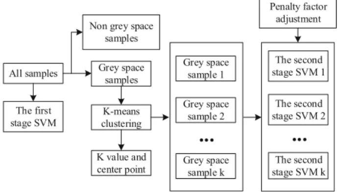
The proposed algorithm is improved for single or mul-tiple SVM by improving the accuracy of single SVM classifier. At the same time, through K-means cluster-ing algorithm and segmented processcluster-ing, the computa-tion requirement of multiple SVM in the second stage is reduced, which improves not only the accuracy but also the training, optimization and classification speed of the model. To solve the issues related to mistaking the unstable conditions of the system as stable ones,

this paper proposes to adjust the penalty factor of the SVM model in the second stage. In addition, adjusting the penalty factor does not change the computation re-quirement of model training and classification. Com-bined with the K-means clustering algorithm, it can reduce the number of unstable state of the system be-ing mistaken for stable ones. The trainbe-ing process of this algorithm is shown in Fig.1.

3.2 First stage SVM

In the first stage of SVM training, it is necessary to ensure the accuracy rate is as high as possible, and to reduce the proportion of samples into the second stage to improve the efficiency of security regions analysis. In this model, Grid Search is adopted first to optimize the parameters of the SVM model, and the SVM model with the best classi-fication accuracy is obtained. The probability output of the SVM is then used to judge the fiducial probability of the sample in the SVM model in the first stage.

The SVM model used here is the RBF kernel, which is shown by the kernel function as:

k xð i;xÞ ¼ exp−γkxi−xk2; γ>0 ð12Þ

In (4) and (12), there are two parameters in the process of parameter optimization: penalty factorCand kernel function parameterγ. The Grid Search method is to give a range of parameter C and γ, divide the grid under the given step size, traverse each point in the grid by cross validation and select the highest accuracy as the optimal parameter. The method of cross validation is to train samples of SVM model in groups, one is used as a real training set and the other is verified by validation set. The most commonly used is the cross validation of N-CV. The method divides samples into N groups, with one group as a test set and the rest as training sets, to evaluate the accuracy of this parameter after all the re-sults are synthesized. After traversing the grid, the classi-fication accuracy of all the parameters is collected.

After selecting the parameters C andγ, the model de-termines the grey space in the sample by the fiducial probability of the classification results of each sample. It then structures the SVM sample set, where xi∈Rm

represents the input characteristics of the sample using active and reactive power of the generators and lines, bus voltage magnitude and phase angle, and active and reactive power of the load as the output characteristics, and y∈{1, 0} represents the classification of the stability output. The function is mapped to the high dimensional space by using the RBF kernel function, and the hyperplane is constructed. The constructor uses the function g(x) to represent the distance between the sample and the optimal hyperplane as

g xð Þ ¼X

l

i¼1

aiyik xð i;xÞ þb ð13Þ

where ai∈Rm is the Lagrange operator and k(xi,x) is

shown in (12).

The distance from the sample to the hyperplane indi-cates the probability of the type of output classification is the sample in. The probability ofy= 0 in this sample is:

P Cð 0jxÞ ¼1= 1þeg xð Þ

ð14Þ

and the probability ofy= 1 in this sample is:

P Cð 1jxÞ ¼1= 1þe−g xð Þ

ð15Þ

The SVM selects the maximum probability between them as the output, and in this model, the maximum probability of the two is selected as the maximum prob-ability of the classification results of the sample. After several experiments, it is known that for samples whose output probability is larger than 0.99, the result is con-sistent with the real stable state. Otherwise, there may be missed or false judgement. Therefore, the sample with SVM output being less than 0.99 will be defined as a grey space sample in the first stage. The samples will be further processed to improve the accuracy of classification.

3.3 K-means clustering

When using K-means clustering to process data in grey space, Euclidean distance is selected as the cluster index. In the sample space, the center points are randomly se-lected for K-means clustering, and the clustering results are observed. After clustering, the appropriate K value and center point are selected. When the K value initially increases, the cluster index declines fast and the clustering effect is improved. However, after the K value increases to a certain degree, the cluster index declines slowly and fur-ther increase of the K value may sometimes even lead to

the increase of the cluster index. This may reach a state of local convergence. In the K-means clustering algorithm, the local optimal condition is eliminated by repeated cal-culation to select the optimal value.

On the choice of the cluster index, the larger the K value is, the smaller the cluster index is and the better effect the clustering has. However, the increase of K value will increase the number of the SVM models in the second stage, the complexity of the model and the amount of required computation. In this model, the K value is selected when the cluster index starts to decline slowly, and the center point of the optimal clustering effect is recorded after repeated calculation.

After a new cluster sample is judged in the grey space by the SVM at the first stage, the Euclidean dis-tance between the sample and each center point is cal-culated. The categories belonging to the sample are determined according to the nearest center point, and the second stage SVM model is used to classify them.

3.4 Second stage SVM

The second stage SVM is used to deal with the grey space data after clustering. According to the conser-vation of the power system, the possibility of the leakage is to be minimized. Thus, a penalty factor is introduced to modify the constraints of the second stage SVM.

In the second stage SVM model, the sample is set as (xi,yi), i= 1, 2, ⋯, l, xi∈Rn. The optimization problem

such as shown in (4) indicates that the first one represents the maximization of the interval between samples, the second one is the slack variable ξi introduced by the existence of deviating points, andCis

the penalty factor. In (4), CP i¼1 n

ξi represents the size of the error term. The greater theCis, the more important it is to represent the error.

The standard C-SVM model uses aCparameter as a penalty factor and does not distinguish between missed and misjudged errors. In order to deal with the situ-ation that the unstable state of power system being mistaken as stable ones, this model selects different penalty factors C1and C0to deal with the distinction

between errors due to different causes. The error term is defined as:

C1 X

i yji¼1

ξiþC0 X

i yji¼0

ξi ð16Þ

min1 2k kw

2_þC 1

X

i yj_i¼1

ξiþC0 X

i yj_i¼0

ξi

s:t: y_i wT_x iþb

≥1−ξi; i¼1;⋯;n ξi≥0; i¼1;⋯;n

ð17Þ

In solving the optimization problem, the Lagrange function is introduced as:

L wð ;b;ξ;α;βÞ ¼1

2k kw

2_þC 1

X

i yj_i¼1

ξiþC0 X

i yj_i¼0

ξi

−X

n

i¼1

aiðyiððwΦð Þxi Þ þbÞ−1þξiÞ−

Xn

i¼1

βiξi

ð18Þ

Being a duality problem, the optimization problem can be changed to:

min

α

1 2

Xn

i¼1 Xn

j¼1

αiαjyiyjk x i;xj−

Xn

i¼1

αi

s:t: Xn

i¼1

y_iαi ¼0

0≤αi≤C1; yi¼1

0≤αi≤C0; yi¼0

ð19Þ

After the solution,α∗can be expressed as:

α_{¼ α}

1;α2;⋯;αn

T

αi∈ð0;C1Þ yi¼1 αi∈ð0;C0Þ yi¼0

_ð

20Þ

Theb∗component is then calculated as:

b_¼y i

Xn

i¼1

y_iαik xð i;xÞ ð21Þ

Finally, a new decision function f(x) is constructed as the classification rule byα∗ and b∗, which are valued by different penalty factors, i.e.

f xð Þ ¼ sgn X

n

i¼1

y_iα

ik xð i;xÞ þb

!

ð22Þ

By increasing the error penalty of theyi= 0 part of the

sample (xi,yi), i.e. the penalty of misjudging the unstable

state, the error of misjudging the unstable states as stable states is reduced.

4 Discussion

4.1 Case study

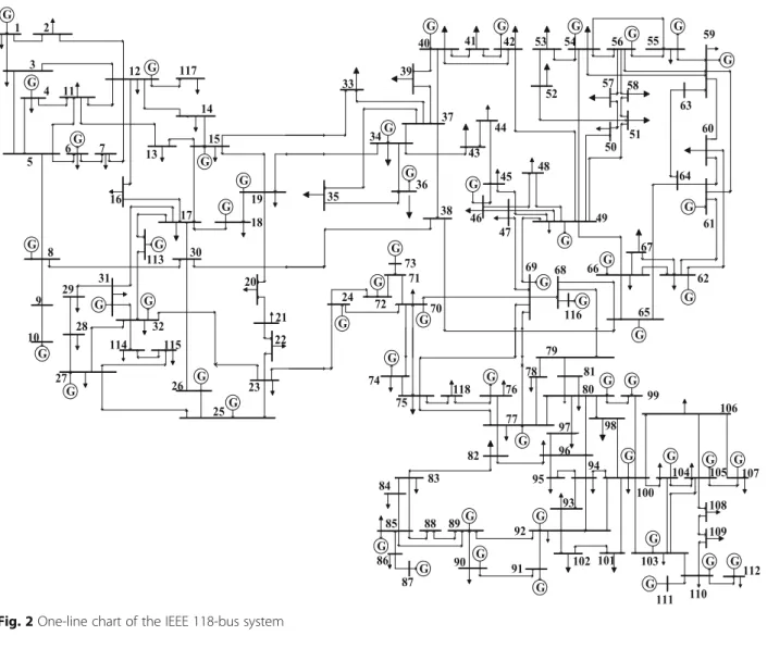
In this paper, the PSAT simulation toolbox is used to carry out power flow calculation and time domain simu-lation. The IEEE 54-machine 118-bus standard test sys-tem is modeled in PSAT, and the single line diagram is shown in Fig.2. The system consists of 3 regions. In an

actual power grid, the lines between regions are usually under heavy load. The fault is located on the interre-gional tie line and the power flow is calculated and sim-ulated in time domain. The stability of the system under the corresponding fault is judged by simulation results. The flow data and stability of the IEEE 118-bus standard test system are used as data set for subsequent data ana-lysis, i.e. the analysis of the system security regions under the corresponding fault. The specific operation is to consider the initial power flow and set the output of each node randomly within ±40% of the rated output, with the load level of the node fluctuating within the range of ±10% of the rated load level. Three-phase short circuit faults are applied in the interregional liaison lines and the faults are cleared after a period of time. The ini-tial power flow of the active and reactive power of the generators and lines, the bus voltage magnitude and phase angle, load active and reactive power at the node, and the final stability of the 54-machine 118-bus system are recorded as the data set. Eight thousand groups of such data are randomly generated as training samples.

In the example test, the fault is applied on the interre-gional connection Line30–38, and the fault setting is shown in Table1.

In the 8000 groups of samples, 6000 groups of data are randomly selected as training samples and the other 2000 groups of data are used as test samples.

First, the parameters of the grid cross validation are optimized and the optimization results of the sample are shown in Fig.3.

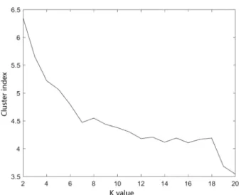
Using the best parameter training, the first stage SVM model is obtained and tested in the test set. The number of samples in the non-gray space area is 807, and the number of samples in the grey space area is 1193 through the sample fiducial probability. The clustering results of grey space samples are tested by repeatedly clustering 10 times to obtain the best clustering effect to avoid local convergence. The variation of cluster index with K value is shown in Fig. 4. As can be seen, the K value of K-means clustering is 9, and 9 s stage SVM are trained by the clustering results.

After clustering analysis and adjusting the penalty factor, the classification effect of the modified SVM model is com-pared with the standard SVM model, as shown in Table2.

Through the example analysis in the IEEE 118-bus, it verifies the effectiveness of the proposed security and stability analysis algorithm in the analysis of the safety regions during faults in the interregional liaison lines.

5 Conclusion

The analysis of the IEEE 118-bus system validates that the proposed model can effectively improve the classifi-cation accuracy of the SVM model. At the same time, the K-means clustering method is used to reduce the sample size of the second stage to improve the training speed of the model.

Through this study, the probability output of SVM can effectively distinguishes the SVM model in gray space. The fiducial probability output of classification results can make the classification results of the vague samples to be effectively recognized for subsequent processing. The classification accuracy of the samples in the gray space can be effectively improved by using

Table 1The fault configuration

Fault Bus

Tripping Line

Failure duration

Stable sample

Unstable sample

Bus38 Line30–38 0.214 s 5846 2154

the clustering analysis with the SVM model. Using the penalty factor adjustment method can reduce the propor-tion of unstable results mistaken as stable ones. In addition, this method can effectively deal with each cluster after being clustered into two samples due to unbalanced training difficulties, so as to improve the accuracy of classification.

Funding

This work was supported by China_’s National key research and development program 2017YFB0902201, National Natural Science Foundation of China under Grant 51777104, Science and Technology Project of the State Grid Corporation of China.

Authors_’contributions

HK carried out the theoretical studies, algorithm guidance and drafted the manuscript. SG participated in the theoretical analysis and guided the research method. WH participated in the research method and simulation analysis. ZL carried out the theoretical studies, algorithm researches and drafted the manuscript. WS participated in the design of the study and performed the simulation analysis. ZQ participated in the design of the model research and performed the simulation analysis. WH conceived of the study, and participated in its design and coordination and helped to draft the manuscript. All authors read and approved the final manuscript.

Competing interests

The authors declare that they have no competing interests.

Author details

1_{Northeast Branch, State Grid Corporation of China, Shenyang 110180, China.} 2_{State Grid Liaoning Electric Power Supply Co. Ltd, Shenyang 110004, China.}

3_{Department of Electrical Engineering, Tsinghua University, Beijing 100084,} China.

Received: 28 December 2017 Accepted: 23 April 2018

References

1. Kundur, P. (1994).Power system stability and control. New York: McGraw-Hill. 2. Weiling, Z., Wei, H., Yong, M., et al. (2016). Conservative online transient

stability assessment in power system based on concept of stability region. Power Syst Technol, 40(4), 992–998.

3. Gomez, F. R., Rajapakse, A. D., Annakkage, U. D., & Fernando, I. T. (2011). Support vector machine-based algorithm for post-fault transient stability status prediction using synchronized measurements.IEEE Trans Power Syst, 26(3), 1474–1483.

4. Zhou, Q., Davidson, J., & Fouad, A. (1994). Application of artificial neural networks in power system security and vulnerability assessment.IEEE Trans Power Syst, 9(1), 525_–532.

5. Al-masri, A., Kadir, M., Hizam, H., & Mariun, N. (2013). A novel implementation for generator rotor angle stability prediction using an adaptive artificial neural network application for dynamic security assessment.IEEE Trans Power Syst, 28(3), 2516_–2525.

6. Amjady, N., & Majedi, S. (2007). Transient stability prediction by a hybrid intelligent system.IEEE Trans Power Syst, 22(3), 1275–1283.

7. Bahbah, A. G., & Girgis, A. A. (2004). New method for generators’angles and angular velocities prediction for transient stability assessment of multimachine power systems using recurrent artificial neural network.IEEE Trans Power Syst, 19(2), 1015–1022.

8. Guo, T., & Milanovic, J. V. (2016). Online identification of power dynamic signature using PMU measurements and data mining [J].IEEE Trans Power Syst, 31(3), 1760–1768.

9. He, M., Vittal, V., & Zhang, J. (2013). Online dynamic security assessment with missing PMU measurements: A data mining approach.IEEE Trans Power Syst, 28(2), 1969_–1977.

10. Sun, K., Likhate, S., Vittal, V., Kolluri, V. S., & Mandal, S. (2007). An online dynamic security assessment scheme using phasor measurements and decision trees.IEEE Trans Power Syst, 22(4), 1935–1943.

11. He, M., Zhang, J., & Vittal, V. (2013). Robust online dynamic security assessment using adaptive ensemble decision-tree leaning.IEEE Trans Power Syst, 28(4), 4089–4098.

12. Li, D. H., & Cao, Y. J. (2006). Power system transient stability analysis based on PMU and hybrid support vector machine.Power Syst Technol, 30(9), 46_–52. 13. Iang, L. X., Wang, X. H., Ang, J. W., et al. (2007). Feature selection for SVM

based transient stability classification.Relay, 35(9), 17–21.

14. Ai, Y. D., Chen, L., Zhang, W. L., et al. (2016). Power system transient stability assessment based on multi-support vector machines.Proc CSEE, 36(5), 1173_–1180. 15. Xu, T., Chiang, H., Liu, G., & Tan, C. (2017). Hierarchical K-means method for clustering large-scale advanced metering infrastructure data. IEEE Trans Power Delivery, 32(2), 609–616.

16. Lin, Y. (2011). Using K-means clustering and parameter weighting for partial-discharge noise suppression.IEEE Trans Power Delivery, 26(4), 2380–2390. Fig. 4Effect of K-means clustering algorithm

Table 2Comparison of classification effect between original SVM and the proposed method

Algorithm GR accuracy Erroneous judgement sample

Missing judgement sample

Classification accuracy

Standard SVM 90.78% 110 70 94.50%