VARIABILITY IN COASTAL SHARK POPULATIONS ACROSS MULTIPLE SPATIOTEMPORAL SCALES
Martin Tomas Benavides
A dissertation submitted to the faculty at the University of North Carolina at Chapel Hill in partial fulfillment of the requirements for the degree of Doctor of Philosophy in the Department
of Marine Sciences in the College of Arts and Sciences.
Chapel Hill 2020
ii © 2020
iii
ABSTRACT
Martin Tomas Benavides: Variability in coastal shark populations across multiple spatiotemporal scales
(Under the direction of F. Joel Fodrie)
Variability across spatiotemporal scales has been recognized by ecologists as a fundamental issue in understanding ecosystem dynamics. Sharks emerged as a conservation concern as their populations declined and their influence on marine ecosystem dynamics became apparent. Efforts to better manage and understand shark populations and their response to anthropogenic pressures have been hindered by a lack of understanding of patterns across multiple scales of time and space. This dissertation aimed to describe patterns of variability in coastal shark populations across multiple spatiotemporal scales.
Chapter 1 exploits a 45-year time series of shark monitoring to describe patterns of
iv
declines in two small coastal shark species, Atlantic sharpnose shark and blacknose shark (Carcharhinus acronotus). These results provide insight on assemblage-level responses to anthropogenic pressure via environmental or genetic mechanisms.
Chapter 3 employs acoustic telemetry to decipher bonnethead shark (Sphyrna tiburo)
v
ACKNOWLEDGEMENTS
Many people influenced this work, too many to make an exhaustive list possible. First and foremost, I would like to thank my advisor and mentor Joel Fodrie, whose incisive intellect and patient guidance I depended on to complete this process. I thank my committee members Pete Peterson, Steve Fegley, Johanna Rosman, and Nate Bacheler for their thoughtful comments that helped focus my dissertation research and develop my thinking as a scientist. I thank my
collaborators Matt Kenworthy, Jeb Byers, Dave Johnston, Amy Yarnall, and Giada Bargione for their critical assistance with fieldwork and data analysis for my dissertation chapters. I thank others who have been immensely helpful in the field or with data sharing/processing, specifically Danielle Keller, Shelby Ziegler, Max Tice-Lewis, Mayor Rett Newton, Julian Dale, Jacob
Krause, Connor Neagle, Austin Moore, and Cameron Luck.
Over the years many have contributed to the UNC-IMS shark survey program and without them this dissertation would not have been possible, above all Dr. Frank Schwartz, whose visionary efforts established the survey and oversaw it for nearly its entirety. I also thank
Captains John Purifoy and Stacy Davis who ran the survey trips during my tenure at UNC-IMS, as well as the UNC-IMS shop crew who ran the gear: Glenn Safrit, Claude Lewis, and Phil Herbst. There were also innumerous undergraduate students, interns, and outside volunteers who assisted me, for which I am deeply grateful.
vi
without which this research would not have been possible. I am also grateful to the UNC Department of Marine Sciences for their support during the admissions process and providing funding during the last year of my dissertation research. Specifically, I would like to thank Marc Alperin, who was instrumental in navigating the admissions process, which was perhaps
uniquely challenging for me due to my scholarship. The UNC-IMS shark survey was funded in its early years by the Carolina Power & Light Company and throughout by the University of North Carolina. I am also grateful to the North Carolina Aquarium Society for funding my research on bonnethead movement and drone surveys. I thank the Atlantic Cooperative Telemetry Network and the FACT Network, and the many members of these networks who shared acoustic telemetry data with me that greatly increased the spatial coverage of my bonnethead tracking efforts.
vii ix x xii 1 5 8 8 10 10 11 14 16 20 35 35 38 38 39
TABLE OF CONTENTS
LIST OF TABLES ………... LIST OF FIGURES ………. LIST OF ABBREVIATIONS AND SYMBOLS ………. INTRODUCTION ………... References ....……….. CHAPTER 1: TEMPORAL PATTERNS OF COASTAL SHARK
COMMUNITY STRUCTURE IN ONSLOW BAY, NORTH CAROLINA ……….... Introduction ....……….... Methods ……….. Field Sampling ……….. Data Analysis ……….... Results ……….... Discussion ……….. References ………... CHAPTER 2: SIZE CHANGES WITHIN A SOUTHEAST UNITED
viii 42 44 51 61 61 63 63 64 66 68 74 91 91 93 93 94 95 97 98 100 105 Results ……….. Discussion ……… References ……… CHAPTER 3: SEASONAL RESIDENCY AND MOVEMENT
PATTERNS OF BONNETHEAD SHARKS (SPHYRNA TIBURO) IN
NORTH CAROLINA AND GEORGIA ESTUARIES ……….. Introduction ……….. Methods ....……… Field Sampling ………... Data Analysis ……….. Results ……….. Discussion ……… References ……… CHAPTER 4: SHARK DETECTION PROBABILITY FROM AERIAL
ix
24 26 27 55 77 78 79 80 81 109 110 LIST OF TABLES
x 28 29 30 31 32 33 34 57 58 59 60 82 83 84 85 86 87 88 89 111 112 113 LIST OF FIGURES
xi
xii
LIST OF ABBREVIATIONS AND SYMBOLS
BOFFFF Big old fat fecund female fish CPUE Catch per unit effort
df Degrees of freedom
FL Fork length
FLa Florida
GA Georgia
L90% 90th percentile of fork length N Number or sample size
NC North Carolina
NIR Near-infrared filter
nMDS Non-metric multidimensional scaling
NOAA National Oceanic and Atmospheric Administration p Probability value
r2 Coefficient of determination
RE Red-edge filter RGB Regular filter
SC South Carolina
SE Standard error
SST Sea surface temperature
TL Total length
xiii
US United States
Χ2 Chi-square value
1
INTRODUCTION
Biological oceanographers have long been aware of the importance of understanding variability across a spectrum of spatiotemporal scales as a fundamental issue in marine
ecological dynamics, first illustrated by Stommel (1963). In deed the concept of pattern and scale in understanding organismal and environmental variability has become a unifying concept in ecology (Haury et al. 1978; Steele 1978; Vance and Doel 2010). An integrated approach to understanding marine ecosystem dynamics emerged, one that coupled the study of biological and physical processes of the oceans across scales (Legendre and Demers 1984). For example, in Legendre (1981), the alternation of stabilization and destabilization of the water column was proposed as a hydrodynamic mechanism conducive to enhancing primary productivity in an estuarine system, accounting for the variability documented on annual scales, such as the spring bloom and subsequent phytoplankton growth (Gilmartin 1964), as well as small-scale turbulence (Savidge 1981). Importantly, however, this tight coupling of biological processes to physical processes for phytoplankton appears to break down at longer timescales (interannual to multidecadal), suggesting the increased variability on these timescales is under the control of other physical mechanisms or perhaps biological mechanisms such as zooplankton grazing (Barton et al. 2015).
2
Weber et al. 1986; Levin 1992). Steele (1978) used the time and space scales of lifespan as a simplistic representation of relevant scales for trophic levels, including phytoplankton,
zooplankton and fish. While useful for illustrating the conceptual problem of observational scale in resolving pattern at successively higher trophic levels, this simplistic depiction may not always be an accurate representation of true trophic dynamics of the system, which could cause the coupling of physical forcing and biological response to occur on widely divergent scales (Denman 1994). Moreover, as recognized by Haury et al. (1978) through the use of a variable time scale in the definition of ambit for long-lived organisms, pattern and its relationship to physical processes will vary depending on the temporal scale of the biological process of interest (e.g., daily foraging, annual migrations, lifetime distribution). For instance, in their study of scale dependent processes of marine birds, Hunt and Schneider (1987) showed that the distribution of birds on meso- to mega-scales (100 - 3,000 km+) is closely related to the presence and
periodicity of upwelling systems (Brown 1979). Conversely, on the coarse-scale (1 – 100 km), concentrations of seabirds appear to be poorly correlated with conditions related to upwelling water masses (see Abrams and Griffiths 1981), with patchiness hypothesized to be related to species-specific responses such as prey preferences and foraging strategy (Schneider and Duffy 1985).
3
(Fulton et al. 2005). Efforts to assess shark populations have been hindered by a paucity of quantitative information and the challenge of reconciling information on a number of relevant spatiotemporal scales to represent species dynamics accurately (Dulvy et al. 2008; Pilling et al. 2009). Understanding patterns in variability of shark populations across a spectrum of
spatiotemporal scales is critical if we are to properly assess and conserve these species; this variability may also serve as a record of ecosystem responses to increasing anthropogenic pressures occurring over a range of scales in time and space. Only one published study has explicitly looked at variability across a broad range of spatiotemporal scales in a shark species, Cetorhinus maximus, which examined correlations of surface sightings with environmental parameters and found basking shark distribution to be determined largely by zooplankton abundance at local scales, whereas at larger scales it was significantly correlated with thermal boundaries characteristic of tidal and shelf-break fronts (Cotton et al. 2005).
Sharks are a group of large, mobile, and generally uncommon species that can make
predicting absolute densities from any single survey approach nearly impossible. An increasing array of emergent technologies can be used in combination with traditional survey approaches to provide new insights in investigations of almost every aspect of shark biology (Carrier et al. 2018). Moreover, each survey approach is particularly suited for sampling at specific scales in time and space. By combining survey approaches there is the potential to synthesize information across spatiotemporal scales. As an example, traditional fishing surveys, suited for gathering long-term data at specific locations, can be combined with acoustic or satellite tracking data that provide potentially greater spatial coverage.
4
5
REFERENCES
Abrams, R., and A. Griffiths. 1981. Ecological structure of the pelagic seabird community in the Benguela Current region. Marine Ecology Progress Series 5:269–277.
Barton, A. D., M. S. Lozier, and R. G. Williams. 2015. Physical controls of variability in north Atlantic phytoplankton communities. Limnology and Oceanography 60(1):181–197. Brown, R. G. B. 1979. Seabirds of the Senegal Upwelling and Adjacent Waters. Ibis 121(3):283–
292.
Carrier, J. C., M. R. Heithaus, and C. A. Simpfendorfer, editors. 2018. Shark research: emerging technologies and applications for the field and laboratory. CRC Press, Boca Raton, FL. Cotton, P. A., D. W. Sims, S. Fanshawe, and M. Chadwick. 2005. The effects of climate
variability on zooplankton and basking shark (Cetorhinus maximus) relative abundance off southwest Britain. Fisheries Oceanography 14(2):151–155.
Denman, K. L. 1994. Scale-determining biological-physical interactions in oceanic food webs. Pages 377–402 in P. S. Giller, A. G. Hildrew, and D. G. Raffaelli, editors. Aquatic ecology: scale, pattern and process. Blackwell Scientific Publications, Oxford.
Dulvy, N. K., J. K. Baum, S. Clarke, L. J. V. Compagno, E. Cortés, A. Domingo, S. Fordham, S. Fowler, M. P. Francis, C. Gibson, J. Martínez, J. A. Musick, A. Soldo, J. D. Stevens, and S. Valenti. 2008. You can swim but you can’t hide: the global status and conservation of oceanic pelagic sharks and rays. Aquatic Conservation: Marine and Freshwater Ecosystems 18(5):459–482.
Fulton, E. A., A. D. M. Smith, and A. E. Punt. 2005. Which ecological indicators can robustly detect effects of fishing? ICES Journal of Marine Science 62(3):540–551.
Gilmartin, M. 1964. The primary production of a British Columbia fjord. Journal of the Fisheries Research Board of Canada 21(3):505–538.
6
Hunt, G. L., and D. C. Schneider. 1987. Scale dependent processes in the physical and biological environment of seabirds. Pages 7–41 in J. P. Croxall, editor. Seabird Feeding Ecology. Cambridge University Press, Cambridge.
Legendre, L. 1981. Hydrodynamic control of marine phytoplankton production: the paradox of stability. Pages 191–207 in J. C. J. Nihoul, editor. Ecohydrodynamics: Proceedings of the 12th International Liège Colloquium on Ocean Hydrodynamics. Elseiver Oceanography Series Volume 32.
Legendre, L., and S. Demers. 1984. Towards dynamic biological oceanography and limnology. Canadian Journal of Fisheries and Aquatic Sciences 41:2–19.
Levin, S. A. 1992. The problem of pattern and scale in ecology: the Robert H. MacArthur Award lecture. Ecology 73(6):1943–1967.
Mackas, D. L., K. L. Denman, and M. R. Abbott. 1985. Plankton patchiness: biology in the physical vernacular. Bulletin of Marine Science 37(2):653–674.
Musick, J. A. 1999. Ecology and conservation of long-lived marine animals. American Fisheries Society Symposium 23:1–10.
Pilling, G. M., P. Apostolaki, P. Failler, C. Floros, P. A. Large, B. Morales-Nin, P. Reglero, K. I. Stergiou, and A. C. Tsikliras. 2009. Assessment and management of data-poor fisheries. Pages 280–305 in A. Payne, J. Cotter, and T. Potter, editors. Advances in Fisheries Science: 50 years on from Beverton and Holt. Blackwell Publishing, Ltd, Oxford.
Savidge, G. 1981. Studies of the effects of small-scale turbulence on phytoplankton. Journal of the Marine Biological Association of the United Kingdom 61(02):477. Cambridge
University Press.
Schneider, D., and D. Duffy. 1985. Scale-dependent variability in seabird abundance. Marine Ecology Progress Series 25:211–218.
Steele, J. H. 1978. Some Comments on Plankton Patches. Pages 1–20 in J. H. Steele, editor. Spatial Pattern in Plankton Communities. Springer, Boston, MA.
7
Vance, T., and R. E. Doel. 2010. Graphical methods and cold war scientific practice: the Stommel diagram’s intriguing journey from the physical to the biological environmental sciences. Historical Studies in the Natural Sciences 40(1):1–47.
Weber, L. H., S. Z. El-Sayed, and I. Hampton. 1986. The variance spectra of phytoplankton, krill and water temperature in the Antarctic Ocean south of Africa. Deep Sea Research Part A, Oceanographic Research Papers 33(10):1327–1343.
8
CHAPTER 1: TEMPORAL PATTERNS OF COASTAL SHARK COMMUNITY STRUCTURE IN ONSLOW BAY, NORTH CAROLINA
Introduction
Understanding how biological communities are organized in time and space and how these patterns are related across scales is perhaps one of the most fundamental challenges for both theoretical and applied ecology (Levin 1992). With increasing global change brought about by anthropogenic pressures such as overexploitation and climate change, being able to detect shared patterns of variation in biological communities and extrinsic influences is an important first step in predicting consequences of these influences (McGowan 1990). Due to their ability to provide historical context or baselines, long-term data sets provide unique insight for disentangling the effects of anthropogenic effects operating on both global scales (e.g., climate change) and local or regional scales (e.g., overfishing), as well as segregating these effects from natural changes (Mieszkowska et al. 2014). Discerning the effects of human pressures, often coupled across scales, is complicated, as illustrated by recent studies suggesting a synergistic effect of climate and exploitation, with top predator removal and concurrent climate change causing complex and cascading top-down effects (Kirby et al. 2009; Planque et al. 2010). In marine ecosystems, sharks could serve as important indicators for system-wide responses to ecological disturbance as a result of their trophic position and relatively sensitive life history characteristics (Fulton et al. 2005).
9
temperatures (Springer 1967; Bres 1993; Heithaus 2004; Knip et al. 2010; Schlaff et al. 2014). For coastal shark species in the Atlantic, these migrations can range up to 3,800 km, a distance traveled by the dusky shark (Carcharhinus obscurus) between the waters off of Long Island, New York and the southwestern Gulf of Mexico (Casey and Kohler 1991). Of the 33 species of Atlantic sharks tagged as part of the National Marine Fisheries Service’s Cooperative Shark Tagging Program between 1962-1993, only the Greenland shark (Somniosus microcephalus) showed no evidence of migration from tag recaptures (Kohler et al. 1998). Understanding coastal shark migrations, and in particular the seasonal windows associated with these migrations, is critical to proper implementation of stock management (Bonfil 1997). Unfortunately, in many instances this information is lacking, depriving management agencies of the information required to coordinate local and regional management efforts (Speed et al. 2010).
10
Methods
Field Sampling
To assess temporal variation in coastal shark community assemblage, I used species-specific time series data generated during the course of a 1973-2018 fishery independent shark survey in Onslow Bay. The survey was conducted by the University of North Carolina at Chapel Hill’s Institute of Marine Sciences (UNC-IMS) and since its inception, the UNC-IMS shark survey has employed standardized longline sampling gear at two fixed stations in Onslow Bay: 4 km
(34.6338°N, 76.6306°W, 15 m depth) and 13 km (34.5512°N, 76.6237°W, 17 m depth) southeast of Beaufort Inlet. During each deployment at each station, a 7.6 mm braided nylon longline extended 1 km, with gangion lines attached to the mainline at every 10 m (N = 100). Each gangion consists of a 1.8 m long, #2-chain leader and a 9/0 Mustad tuna J hook. Polyball buoys are attached between every 10 gangions (100-m separation), allowing the longline gear to fish the entire water column at each station.
In addition to standardized gears and stations, consistent deployment methods have been used since the first sets were made in 1973. Survey trips are conducted biweekly, between April and November each year, on 10-15-m research vessels operated by UNC-IMS. A demersal trawl is used at the start of each survey day to collect bait (e.g., spot Leiostomus xanthurus, Atlantic croaker Micropogonias undulatus), which are attached subsequently through the operculum onto hooks (one fish per hook). Longline deployment occurs between 0800 and 1300 hours, with the
11
for fork length (FL) and total length to the nearest mm. Live individuals are outfitted with an external dart tag and returned to the water (~90% of catch). The survey is conducted under UNC-IMS Institutional Animal Care and Use Committee protocol 19-137.0.
Data Analysis
I selected 12 of the 21 shark species caught in the survey for seasonality analyses generally based on large overall sample sizes (N > 100 individuals captured): blacknose shark
(Carcharhinus acronotus), spinner shark (Carcharhinus brevipinna), silky shark (Carcharhinus falciformis), finetooth shark (Carcharhinus isodon), blacktip shark (Carcharhinus limbatus), dusky shark, sandbar shark (Carcharhinus plumbeus), smooth dogfish (Mustelus canis), Atlantic sharpnose shark (Rhizoprionodon terraenovae), and scalloped hammerhead shark (Sphyrna lewini). Two species had lower sample sizes (bull shark Carcharhinus leucas, N = 26; tiger shark Galeocerdo cuvier, N = 46), but were added due to being large coastal sharks of general public interest. For each focal species, I evaluated catch per unit effort (CPUE) from all samples with non-zero catch (due to zero-inflation) as a function of day of year, as well as SST measurements taken during the survey, to reveal any seasonal trends or correlation with SST in the catch data. Visual inspection of abundances allowed me to categorize species for seasonality as
spring/autumn (bimodal annual peaks in CPUE with absence during summer months) or summer (single annual peak in CPUE during summer months). Monthly mean CPUE values were
12
the maximum mean CPUE value. This index was examined across the 12 focal species to look for patterns of seasonal succession or turnover in community assemblage.
To better understand how temperatures might be associated with different months of the year, I explored mean SST as a function of month. I also fit Gaussian curve models to CPUE data as a function of SST, using the ‘nls2sol’ algorithm from the Port library
(https://netlib.sandia.gov/port/), to determine how the appearance or disappearance of particular species might be related to seasonal temperature changes. These models were used to calculate the inflection points (mean + 1 standard deviation) to infer temperatures associated with periods of entrance and exit for each species. Only the lower-temperature inflection point was utilized for non-seasonal and summer seasonal species since they both entered and exited during colder temperatures. Conversely, for spring/autumn seasonal species, both inflection points were utilized, since they first exited as waters warmed in summer, returning again in milder autumn months before their final exit. Model fit was assessed visually and using p-values of t-tests for model parameters (mean, standard deviation). Models that failed to converge, surpassed a p-value of 0.1 for any parameter, or failed to accurately represent the data based on visual inspection (i.e., where a majority of data points fell outside the range of the Guassian curve) were not utilized.
13
effort between days and allow for correlation with SST. For both daily and yearly aggregations I calculated mean SST across longline sets within each grouping, for use in correlation analyses.
14
To examine for changes in seasonal community assemblage on decadal time scales, I parsed CPUE data, using the clusters from my annual mean CPUE nMDS analysis. These data were then aggregated as mean CPUE, binned by month, and frequency of occurrence was calculated for each species as the proportion of the total monthly mean CPUE across species. All statistical analyses were performed in R (R Core Team 2016).
Results
The UNC-IMS shark survey database consisted of a total of 596 trips with 1,134 longline sets made using 142,505 baited hooks and 9,266 individual sharks captured across 21 species (Table 1.1). Atlantic sharpnose shark, blacknose shark, dusky shark, and blacktip shark were
numerically dominant in terms of raw abundance, representing 77% of the catch (Atlantic sharpnose shark – 40%, blacknose shark – 16%, dusky shark – 11%, blacktip shark – 10%). Individuals from the 21 species caught in the survey ranged in size from 215-2860 mm in FL and represented eight distinct management groupings (Table 1.2).
15
Spring/autumn species were mostly absent from catches during July and August, before reappearing in September or October (Figure 1.2).
Monthly mean temperatures first climbed from 17.6 °C in April to 28 °C in August, before dropping back to 18.7 °C by November (Figure 1.3). Patterns of CPUE as a function of SST were similar among species, with all focal species exhibiting unimodal distributions of CPUE,
although the temperature at which these peaks occurred, as well the distribution of points along the temperature axis varied (Figure 1.4). Entrance and exit periods for spring/autumn species were associated with temperatures of 14.2-17.2 °C for first entrance and last exit, as well as
21.3-26.4 °C for first exit and second entrance (p < 0.01), although the model for silky shark was rejected upon visual inspection of model fit to data. Summer species (excluding bull shark and tiger shark) displayed entrance and exit temperatures of 19-27.3 °C, although model fit was not
statistically clear in the case of blacktip shark and spinner shark (p < 0.1). Models for tiger shark and bull shark were rejected due to failure to converge and lack of statistical clarity (p > 0.5), respectively (Table 1.3).
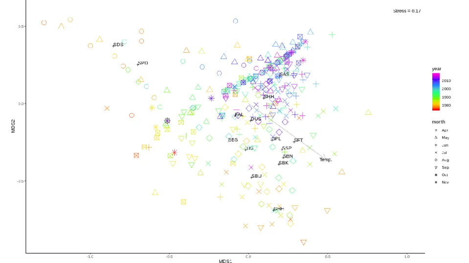
Community structure based on multivariate analysis of daily mean CPUE resulted in temporal patterns on both seasonal (shapes of points) and interannual (color of points) time scales, which could be related to specific species based on weighted average scores (Figure 1.5). Temperature was clearly correlated with dissimilarity in community structure along the first and second order axes (r2 = 0.37; p = 0.001; Figure 1.5). For community structure based on
16
Community assemblage was dominated by spring/autumn and summer species during the early years of the survey that corresponded to the first nMDS cluster group (1973-1989). During the years corresponding to the second nMDS cluster (1990-2018) Atlantic sharpnose shark became the dominant species in all months except April, which was still dominated by smooth dogfish (Figure 1.7).
Discussion
This study analyzed the longest running shark survey program conducted on the US Atlantic coast to characterize temporal patterns in a diverse assemblage of sharks across multiple time scales and establish a baseline for future studies. Moreover, my analyses show that community structure is correlated with temperature changes on seasonal and perhaps interannual time scales. These data also provide a window into long-term change in the coastal shark community of Onslow Bay, showing an already altered baseline and the potential for future shifts in seasonal community composition as a result of climate change.
17
community structure and distribution patterns, which this study supports (Ulrich et al. 2007; Froeschke et al. 2010; Ward-Paige et al. 2015; Plumlee et al. 2018).
CPUE annual patterns of the 12 focal species revealed a transition between spring/autumn and summer species at a threshold of approximately 25 °C. The patterns revealed in the individual species scatterplots of CPUE as a function of time (day of year), as well as the monthly CPUE indices for all 12 species, suggest there is clearly definable seasonal turnover in the community assemblage (Figures 1.1 & 1.2). This appears to be correlated to temperature, as indicated by the calculations of periods of entrance and exit for each species as a function of SST, which align with the range of monthly mean temperatures during months that each species is observed (Table 1.3; Figures 1.1 & 1.3). Furthermore, the range of temperatures associated with periods of first exit in spring/autumn species (21.3-26.4 °C) roughly coincides with the range of temperatures associated with periods of entrance for summer species (19-27.3 °C), with a majority of the species turnover having taken place when temperatures reach 25-26 °C (Table 1.3). Whereas previous work found that spring/autumn species (e.g., sandbar sharks) remained throughout summer months, I found that they were absent, which could be caused by differing sampling methodologies, with other studies sampling estuarine waters (Schwartz 2003; Ulrich et al. 2007; Drymon et al. 2010). Temperature thresholds have been hypothesized to stimulate migration in coastal sharks, often to or from nursery areas in estuarine waters, which may explain the discrepancy in results for sandbar sharks (e.g., Grubbs et al. 2007; Heupel 2007).
18
survey period could continue to be numerically dominant (Figures 1.6 & 1.7). Two other meta analyses of survey data from these regions found population increases in Atlantic sharpnose shark on decadal timescales and attributed these to mesopredatory release as a result of the overfishing of large coastal sharks and implementation of bycatch reduction devices,
mechanisms which could explain the dominance of this species (Myers et al. 2007; Peterson et al. 2017). In that context, the results of this study underscore the need for future, targeted studies to resolve potential causes of the rise in Atlantic sharpnose shark populations. Concurrently, I suggest clues to predicting future shifts as a result of climate change can be found on seasonal time scales, where if observed seasonal migration onsets/endpoints correlated with temperature changes continue to hold, I would hypothesize that all species would begin to show up slightly earlier in the year and stay later as water temperatures warm earlier and stay warm later. This could favor summer species to become more numerically dominant, as they expand their seasonal presence.
19
each species I chose to remove zero-catch data when examining seasonal patterns in the 12 focal species. I also used the delta approach, however, modeling presence/absence and abundance data separately and then combining these estimates (sensu Serafy et al. 2007), and seasonal patterns were nearly identical to those reported here when incorporating zero-catch data.
20
REFERENCES
Bonfil, R. 1997. Status of shark resources in the southern Gulf of Mexico and Caribbean: implications for management. Fisheries Research 29(2):101–117.
Bray, J. R., and J. T. Curtis. 1957. An ordination of the upland forest communities of southern Wisconsin. Ecological Monographs 27(4):325–349.
Bres, M. 1993. The behaviour of sharks. Reviews in Fish Biology and Fisheries 3(2):133–159. Cao, Y., D. P. Larsen, and R. S.-J. Thorne. 2001. Rare species in multivariate analysis for
bioassessment: some considerations. Journal of the North American Benthological Society 20(1):144–153.
Casey, J. G., and N. E. Kohler. 1991. Long distance movements of Atlantic sharks. Pages 87–91 in S. H. Gruber, editor. Discovering sharks, 1st edition. American Littoral Society,
Highlands, NJ.
Clarke, K. R., P. J. Somerfield, and M. G. Chapman. 2006. On resemblance measures for ecological studies, including taxonomic dissimilarities and a zero-adjusted Bray–Curtis coefficient for denuded assemblages. Journal of Experimental Marine Biology and Ecology 330(1):55–80.
Drymon, J. M., S. P. Powers, J. Dindo, B. Dzwonkowski, and T. A. Henwood. 2010.
Distributions of sharks across a continental shelf in the northern Gulf of Mexico. Marine and Coastal Fisheries 2(1):440–450.
Faith, D. P., P. R. Minchin, and L. Belbin. 1987. Compositional dissimilarity as a robust measure of ecological distance. Vegetatio 69(1–3):57–68.
Froeschke, J., G. Stunz, and M. Wildhaber. 2010. Environmental influences on the occurrence of coastal sharks in estuarine waters. Marine Ecology Progress Series 407:279–292.
21
Grubbs, R. D., J. A. Musick, C. L. Conrath, and J. G. Romine. 2007. Long-term movements, migration, and temporal delineation of a summer nursery for juvenile sandbar sharks in the Chesapeake Bay region. American Fisheries Society Symposium 50:87–107.
Harley, S. J., R. A. Myers, and A. Dunn. 2001. Is catch-per-unit-effort proportional to abundance? Canadian Journal of Fisheries and Aquatic Sciences 58: 1760–1772.
Heithaus, M. R. 2004. Predator-prey interactions. Pages 487–521 in J. C. Carrier, J. A. Musick, and Heith, editors. Biology of sharks and their relatives. CRC Press LLC, Boca Raton, FL. Heupel, M. R. 2007. Exiting Terra Ceia Bay: examination of cues stimulating migration from a
summer nursery area. American Fisheries Society Symposium 50:265–280.
Kirby, R. R., G. Beaugrand, and J. A. Lindley. 2009. Synergistic effects of climate and fishing in a marine ecosystem. Ecosystems 12(4):548–561.
Knip, D., M. Heupel, and C. Simpfendorfer. 2010. Sharks in nearshore environments: models, importance, and consequences. Marine Ecology Progress Series 402:1–11.
Kohler, N. E., J. G. Casey, and P. A. Turner. 1998. NMFS cooperative shark tagging program, 1962-93: an atlas of shark tag and recapture data. Marine Fisheries Review 60(2):1.
Levin, S. A. 1992. The problem of pattern and scale in ecology: the Robert H. MacArthur Award lecture. Ecology 73(6):1943–1967.
McGowan, J. A. 1990. Climate and change in oceanic ecosystems: the value of time-series data. Trends in Ecology and Evolution 5(9):293–299. Elsevier Current Trends.
Mieszkowska, N., H. Sugden, L. B. Firth, and S. J. Hawkins. 2014. The role of sustained observations in tracking impacts of environmental change on marine biodiversity and ecosystems. Philosophical Transactions of the Royal Society A 372:20130339.
Myers, R. A., J. K. Baum, T. D. Shepherd, S. P. Powers, and C. H. Peterson. 2007. Cascading effects of the loss of apex predatory sharks from a coastal ocean. Science 315(5820):1846– 1850.
22
Office of Sustainable Fisheries, Highly Migratory Species Management Division, Silver Spring, MD.
Oksanen, J., F. G. Blanchet, M. Friendly, R. Kindt, P. Legendre, D. McGlinn, P. R. Minchin, R. B. O’Hara, G. L. Simpson, P. Solymos, M. H. H. Stevens, E. Szoecs, and H. Wagner. 2019. vegan: community ecology package. https://cran.r-project.org/package=vegan.
Peterson, C. D., C. N. Belcher, D. M. Bethea, W. B. Driggers, B. S. Frazier, and R. J. Latour. 2017. Preliminary recovery of coastal sharks in the south-east United States. Fish and Fisheries 18(5):845–859.
Planque, B., J. M. Fromentin, P. Cury, K. F. Drinkwater, S. Jennings, R. I. Perry, and S. Kifani. 2010. How does fishing alter marine populations and ecosystems sensitivity to climate? Journal of Marine Systems 79(3–4):403–417.
Plumlee, J. D., K. M. Dance, P. Matich, J. A. Mohan, T. M. Richards, T. C. TinHan, M. R. Fisher, and R. J. D. Wells. 2018. Community structure of elasmobranchs in estuaries along the northwest Gulf of Mexico. Estuarine, Coastal and Shelf Science 204:103–113.
R Core Team. 2016. R: A language and environment for statistical computing. http://www.r-project.org.
Schlaff, A. M., M. R. Heupel, and C. A. Simpfendorfer. 2014. Influence of environmental factors on shark and ray movement, behaviour and habitat use: a review. Reviews in Fish Biology and Fisheries 24(4): 1089–1103.
Schwartz, F. J. 2003. Sharks, skates, and rays of the Carolinas. The University of North Carolina Press, Chapel Hill, North Carolina.
Serafy, J. E., M. Valle, C. H. Faunce, and J. Luo. 2007. Species-specific patterns of fish abundance and size along a subtropical mangrove shoreline: an application of the delta approach. Bulletin of Marine Science 80(3): 609–624.
23
Springer, S. 1967. Social organization of shark populations. Pages 149–174 in P. W. Gilbert, R. F. Matthewson, and D. P. Rall, editors. Sharks, skates, and rays. The John Hopkins Press, Baltimore, MD.
Ulrich, G. F., C. M. Jones, W. B. Driggers, J. M. Drymon, D. Oakley, and C. Riley. 2007. Habitat utilization, relative abundance, and seasonality of sharks in the estuarine and nearshore waters of South Carolina. American Fisheries Society Symposium 50:125–139.
Ward, P. 2008. Empirical estimates of historical variations in the catchability and fishing power of pelagic longline fishing gear. Reviews in Fish Biology and Fisheries 18:408–426. Ward-Paige, C. A., G. L. Britten, D. M. Bethea, and J. K. Carlson. 2015. Characterizing and
24
Table 1.1: Summary of effort, date range, temperature and species-specific catch for each year of UNC-IMS survey. Temperature is shown as mean + 1 standard error. Catch is listed as raw catch for each species.
Year Survey
trips Longline sets Hooks Date range (day of
year)
Temperature
(°C) sharpnose Atlantic thresher Bigeye Blacknose Blacktip Bull Dusky Finetooth
1973 6 11 980 170-276 NA 9 0 40 26 3 6 0
1974 9 17 1660 108-284 NA 5 0 21 15 1 70 0
1975 15 26 2527 122-322 18 17 0 62 50 3 123 0
1976 15 26 2192 106-307 20.7 + 1.2 7 0 37 29 0 52 0 1977 16 30 2868 109-314 23.8 + 1.3 20 0 134 34 1 78 1 1978 14 26 2382 102-311 22.1 + 0.8 31 0 61 39 0 12 1 1979 15 29 3129 93-303 23.4 + 0.7 31 0 71 22 4 32 3 1980 15 29 4953 94-288 22.3 + 1.2 60 0 85 83 0 93 0 1981 16 31 4267 105-300 23.2 + 1 31 0 29 12 0 75 1 1982 16 32 5533 110-328 22.8 + 1 16 0 65 33 4 116 2 1983 16 31 5175 111-319 23.2 + 0.9 69 0 33 62 2 51 2 1984 17 34 5340 110-304 24.6 + 0.6 44 0 79 83 1 81 0 1985 16 30 4624 122-301 24.5 + 0.6 77 0 43 23 0 18 0 1986 15 29 4601 104-314 21.1 + 2.1 50 0 24 40 0 35 0 1987 13 25 4369 117-292 26.8 + 0.9 81 0 48 80 0 54 2 1988 17 42 6217 109-291 25 + 0.8 151 0 127 50 0 31 6 1989 16 36 6370 100-289 25 + 0.7 67 0 40 25 0 33 17 1990 15 29 4655 106-302 26 + 0.6 60 0 15 2 0 3 0 1991 14 27 3925 105-302 25.7 + 0.8 86 0 31 29 2 13 0 1992 12 23 3080 118-301 24.3 + 0.9 121 0 45 7 0 0 4 1993 11 21 3090 137-299 27.2 + 0.6 126 0 49 13 1 4 3
1994 15 30 4102 108-304 NA 78 0 32 33 0 11 46
25
Great hammer
head
Lemon Night Nurse Sand
tiger Sand-bar Scalloped hammer-head
Silky Smooth
dogfish hammerSmooth head
Spin-ner Spiny dog-fish
Tig-er White
0 1 0 0 0 0 16 0 0 1 0 0 2 0
0 0 2 2 0 0 9 0 42 0 4 0 1 1
2 0 0 0 0 6 34 0 2 1 6 0 2 0
0 0 0 0 0 2 30 0 20 0 2 0 0 0
1 0 0 0 0 33 36 0 44 0 12 0 1 0
0 0 0 0 1 29 21 0 43 0 20 3 1 0
0 1 0 0 0 36 27 1 62 0 27 5 9 0
0 0 0 0 0 1 45 1 54 0 9 0 4 0
0 0 0 0 0 3 34 0 69 0 2 0 1 0
0 0 0 0 0 4 23 19 27 0 8 0 2 0
0 0 0 0 0 43 34 31 36 0 7 0 1 0
0 0 0 0 0 17 40 12 32 0 2 0 2 0
0 0 0 0 0 19 10 3 4 0 1 0 2 0
0 0 0 0 0 10 14 25 1 0 3 0 3 0
0 0 0 0 0 43 19 16 30 0 12 0 3 0
0 0 0 0 0 17 37 30 6 0 10 0 0 0
0 0 0 0 0 15 4 18 21 1 11 2 0 0
0 0 0 0 0 0 1 5 20 0 0 0 1 0
0 0 0 0 0 2 1 4 7 0 12 1 0 0
0 0 0 0 0 2 1 1 4 0 5 0 0 0
0 0 0 0 0 2 3 1 4 0 4 0 1 0
0 0 0 0 0 24 3 4 2 1 12 0 0 0
1 0 0 0 0 1 0 1 7 0 7 0 0 0
0 0 0 0 0 1 3 2 3 0 14 0 0 0
1 0 0 0 0 3 0 0 0 0 7 0 0 0
0 0 0 0 0 3 1 8 2 0 4 0 1 0
0 0 0 0 0 2 1 0 0 0 9 0 0 0
0 0 0 0 0 1 4 1 3 0 6 0 0 0
0 0 0 0 0 0 1 0 0 0 2 0 0 0
0 0 0 0 0 0 2 1 1 0 0 0 1 0
0 0 0 0 0 0 2 6 3 0 6 0 0 0
0 0 0 0 0 0 2 0 6 0 3 0 0 0
0 0 0 0 0 0 4 2 5 0 5 0 0 0
0 0 0 0 0 1 13 3 6 0 8 0 0 0
0 0 0 0 0 0 8 1 2 0 2 0 1 0
0 0 0 0 0 1 6 0 2 0 0 0 0 0
0 0 0 0 1 0 0 0 0 0 0 0 0 0
0 0 0 0 1 0 2 2 0 4 1 0 0 0
0 0 0 0 0 0 10 1 0 0 10 0 0 0
0 0 0 0 0 0 3 0 0 0 3 0 0 0
0 0 0 0 0 0 12 0 0 0 2 0 0 0
0 0 0 0 0 0 3 0 1 0 11 0 1 0
0 0 0 0 0 0 5 0 1 0 0 1 1 0
0 0 0 0 0 0 3 0 0 0 6 0 3 0
0 0 0 0 0 0 4 0 0 0 0 0 1 0
26
Table 1.2: Summary of coastal shark species; longline CPUE (mean + standard error); FL = fork length, f = female, m = male; management grouping according to NMFS 2006; individuals for which sex was not recorded were omitted for sex ratio calculations.
Species N CPUE (sharks/100
hooks) FL Range (mm) Sex Ratio (f:m) Management Atlantic sharpnose 3690 2.734 + 0.114 215-1315 1689:1936 Non-blacknose
small coastal
Bigeye thresher 1 0.001 + 0.001 2860 1:0 Prohibited
Blacknose 1472 0.988 + 0.072 270-1850 289:175 Blacknose Blacktip 940 0.58 + 0.045 320-2000 343:549 Aggregated
large coastal
Bull 26 0.018 + 0.004 390-2370 2:9 Aggregated
large coastal Dusky 1035 0.697 + 0.09 215-2550 283:220 Prohibited Finetooth 114 0.068 + 0.017 740-1350 15:41 Non-blacknose
small coastal Great hammerhead 5 0.004 + 0.002 1640-2390 1:3 Hammerhead
Lemon 2 0.002 + 0.001 2160 0:1 Aggregated
large coastal
Night 2 0.002 + 0.059 NA 1:0 Prohibited
Nurse 2 0.001 + 0.001 1660-2073 0:2 Aggregated
large coastal Sand tiger 3 0.003 + 0.002 1550-1980 0:2 Prohibited
Sandbar 323 0.231 + 0.031 455-2290 283:220 Aggregated large coastal (research only) Scalloped
hammerhead 535 0.374 + 0.03 590-3048 229:270 Hammerhead
Silky 199 0.11 + 0.02 280-1600 108:89 Aggregated
large coastal Smooth dogfish 573 0.487 + 0.07 290-1500 16:9 Smoothhound Smooth hammerhead 8 0.006 + 0.003 840-1900 3:2 Hammerhead Spinner 277 0.204 + 0.023 600-2110 79:53 Aggregated
large coastal Spiny dogfish 12 0.01 + 0.005 640-950 12:0 Spiny dogfish
Tiger 46 0.032 + 0,006 710-2510 4:1 Aggregated
large coastal
27
Table 1.3: Summary of seasonality (summer or spring/autumn), first entrance/exit sea surface temperature (SST) for each of the 12 focal species, and second entrance/exit for sprin/autumn seasonal species. Species for which no convergence was found or for which model fit was deemed inappropriate were removed from entrance SST and exit SST calculations.
Species Seasonality 1st entrance/exit SST (°C) 2nd entrance/exit SST (°C) Atlantic sharpnose
shark 3 season 15.2 NA
Blacknose shark summer 25 NA
Blacktip shark summer 25.6 NA
Bull shark summer NA NA
Dusky shark spring/autumn 17.2 25.4
Finetooth shark summer 27.3 NA
Sandbar shark spring/autumn 17 26.4
Scalloped hammerhead shark
summer 21.6 NA
Silky shark spring/autumn NA NA
Smooth dogfish spring/autumn 14.2 21.3
Spinner shark summer 19 NA
Figure 1.1: Scatterplots of CPUE by day of year for each of the 12 focal species. Axis for day of year has been converted to monthly scale to aid in interpretation.
Figure 1.2: Heat map of CPUE index for each of 12 focal species across survey months. Index is calculated as monthly mean CPUE/ maximum of monthly mean CPUE values for each species.
30
Figure 1.4: Scatterplots of CPUE by SST for each of the 12 focal species with guassian curve model fits and entrance/exit
temperature calculations plotted as vertical lines. Species for which no convergence was found or for which model fit was deemed inappropriate are shown simply as scatterplots.
Figure 1.5: nMDS plot of daily mean CPUE and fitted vector for SST (Temp.). Three letter codes indicate weighted average points for each species. Colors represent year, while shapes represent month. Species codes (N = 15): DUS, dusky shark (Carcharhinus
obscurus); FAL, silky shark (Carcharhinus falciformis); GHH, great hammerhead shark (Sphyrna mokarran); SAS, Atlantic sharpnose shark (Rhizoprionodon terraenovae); SBK, blacktip shark (Carcharhinus limbatus); SBN, blacknose shark (Carcharhinus acronotus); SBS, sandbar shark (Carcharhinus plumbeus); SBU, bull shark (Carcharhinus leucas); SDS, smooth dogfish (Mustelus canis); SFT, finetooth shark (Carcharhinus isodon); SHH, smooth hammerhead (Sphyrna zygaena); SPD, spiny dogfish (Squalus acanthias); SPL, scalloped hammerhead shark (Sphyrna lewini), SSP, spinner shark (Carcharhinus brevipinna); TIG, tiger shark (Galeocerdo cuvier).
Figure 1.6: nMDS plot of annual mean CPUE. Colors represent clusters drawn at 10% similarity.
Figure 1.7: Stacked bar plots showing frequency of occurrence for mean CPUE values of each species aggregated by month. Top bar plot corresponds to annual mean nMDS cluster group 1 (1973-1989), while bottom bar plot corresponds to annual mean nMDS cluster group 2 (1990-2018). Species codes (N = 21): BTH, bigeye thresher (Alopias superciliosus); DUS, dusky shark (Carcharhinus
obscurus); FAL, silky shark (Carcharhinus falciformis); GHH, great hammerhead shark (Sphyrna mokarran); LEM, lemon shark (Negaprion brevirostris); SAS, Atlantic sharpnose shark (Rhizoprionodon terraenovae); SBK, blacktip shark (Carcharhinus limbatus); SBN, blacknose shark (Carcharhinus acronotus); SBS, sandbar shark (Carcharhinus plumbeus); SBU, bull shark (Carcharhinus leucas); SDS, smooth dogfish (Mustelus canis); SFT, finetooth shark (Carcharhinus isodon); SHH, smooth hammerhead (Sphyrna zygaena); SNI, night shark (Carcharhinus signatus); SNR, nurse shark (Ginglymostoma cirratum); SPD, spiny dogfish (Squalus acanthias); SPL, scalloped hammerhead shark (Sphyrna lewini), SSP, spinner shark (Carcharhinus brevipinna); TIG, tiger shark (Galeocerdo cuvier); WSH, white shark (Carcharodon carcharias).
35
CHAPTER 2: SIZE CHANGES WITHIN A SOUTHEAST UNITED STATES COASTAL SHARK ASSEMBLAGE
Introduction
Fishing can cause substantial changes within exploited fish populations, both as a result of selective removal of target species and bycatch of non-target species. Size-selective harvesting (either targeted or bycatch fishes, which is the process of differentially removing larger
individuals of a particular species due to gear design (e.g., net mesh size) or management
directive (e.g., minimum size limits), has been documented across diverse fishes, often leading to a reduction in mean or maximum observed body size within a stock (Fenberg and Roy 2008). Truncation of size structure towards smaller individuals is troubling on both economic and ecological levels. Growth overfishing - the harvesting of fish before they reach their growth potential - results in decreased yield-per-recruit, was the first form of overfishing to be
36
There are multiple, somewhat competing mechanistic hypotheses regarding the response of fished species to harvest pressure vis-à-vis population-level size structure. Darwinian fisheries science has focused on the potential of harvest pressure to select for traits such as reduced growth or earlier size- or age-at-maturity (Law 2007). In size-selective fisheries targeting large individuals, fish growing more quickly or reproducing at larger sizes and older ages may be captured before successfully contributing to the spawning population, greatly reducing their individual fitness relative to slower growers or earlier reproducers (Ratner and Lande 2001; Conover and Munch 2002). Over evolutionary scales, this could truncate the size structure of an exploited population towards smaller fish. Alarmingly, these potential evolutionary consequences may be hard to reverse with the relaxation of fishing pressure due to hysteresis, or a lag
associated with relatively weak selection differentials in the opposing direction (Allendorf and Hard 2009). While evolutionary dynamics may drive fished populations towards smaller individuals, environmental selection within exploited stocks could have the opposite effect on fish. Reduction of stock abundance can cause a release from intraspecific competition, resulting in greater per-capita availability of resources and increased growth, as has also been documented in a number of marine fishes (Heino and Godo 2002). These latter observations support the hypothesis that such density-dependent growth could lead to an increase in body size of individuals through time via compensatory processes in harvested populations (Hilborn and Minte-vera 2008).
37
fished taxa/stocks, however, is the fundamental need to document patterns in size-based indicators over appropriate timescales (i.e., years to decades) to guide us in understanding the dynamics and root mechanisms of size-structure shifts (Shin et al. 2005). Sharks are an
interesting and important test case for evaluating changes in size structure, as there are a mix of factors that might buffer or exacerbate harvest-driven changes. Within this group, many species are defined by relatively K-selected life histories (i.e., slower growth, larger maximum size, longer maximum age, lower fecundity), and as such are vulnerable to overfishing (Stevens et al. 2000). The effects of maternal investment on offspring in sharks has received relatively limited attention and has yet to be fully explored; however, there is evidence suggesting that maternal size can affect both offspring quantity (litter size) and quality (fitness) (Carlson and Baremore 2003; Hussey et al. 2010; Baremore and Passerotti 2013). Gears used to harvest sharks include those that are likely to be size selective (i.e., gill nets), but also some that are potentially less so (i.e., long lines) (Hovgård and Lassen 2000; ASMFC 2008). Because shark species are
38
rays, which could further complicate the patterns of size structure within some fished species such as blacknose shark (sensu Myers et al. 2007).
With these dynamics in mind, we used a decades-running survey of the coastal shark assemblage in Onslow Bay, North Carolina, to document temporal patterns of population size structure among 12 commonly captured species. Our overarching goal was to evaluate the null hypothesis that size-structure has not changed appreciably over time, on a species-by-species basis. Observed patterns are discussed in the context of management strategies, potential genetic and environmental drivers of size structure within fished populations, and purported
“mesopredator release”.
Methods
Field sampling
To examine trends in size structure within coastal shark populations, we used species-specific time series size data generated during the course of a 1972-present fishery independent shark survey in Onslow Bay, North Carolina. The survey was conducted by the University of North Carolina at Chapel Hill’s Institute of Marine Sciences (UNC-IMS) and since its inception, the UNC-IMS shark survey has employed standardized longline sampling gear at two fixed stations in Onslow Bay: 4 km (34.6338°N, 76.6306°W, 15 m depth) and 13 km (34.5512°N, 76.6237°W, 17 m depth) southeast of Beaufort Inlet. During each deployment at each station, the 7.6 mm braided nylon longline extends 1 km, with gangion lines attached to the mainline at every 10 m (N = 100). Each gangion consists of a 1.8 m long, #2-chain leader and a 9/0 Mustad tuna J hook. Polyball buoys are attached between every 10 gangions (100-m separation), allowing the
39
In addition to standardized gears and stations, consistent deployment methods have been used since the first sets were made in 1972. Survey trips were conducted biweekly, between April and November each year, on 10-15-m research vessels operated by UNC-IMS. A demersal trawl was used at the start of each survey day to collect bait (e.g., spot Leiostomus xanthurus, Atlantic croaker Micropogonias undulatus), which were attached through the operculum on hooks (one fish per hook). Longline deployment occurred between 0800 and 1300 hours, with
the gear soaked for one hour during each set. Efforts were made to deploy at each station on each survey day (weather dependent), and the inshore set was typically, but not always, made first. Upon gear recovery, all captured sharks were identified to species, sexed, and measured for fork length (FL) and total length (TL) to the nearest mm. Live individuals were outfitted with an external dart tag and returned to the water (~90% of catch). To date, more than 500 survey trips have been conducted, > 1,000 longline sets have been made, > 100,000 baited hooks have been set, and > 10,000 individual shark captures across 21 species have contributed to the UNC-IMS shark survey database. The survey is conducted under UNC-IMS Institutional Animal Care and Use Committee protocol 19-137.0.
Data Analysis
40
For each focal species, separately, we binned data by year, combining individuals across all months and both stations to describe the entire surveyed population. We utilized FL data as this measurement was the most consistently collected across the entire survey, and we focused on data collected during 1975 – 2018 since data from the first three survey years reported abundance and TL more heavily, rather than FL. For each species*year, we then used three different size indices to obtain a more holistic and robust assessment of potential size changes over time: mean FL, median FL, and an index of maximum FL (L90% or 90th percentile of FL).
The advantage of using the mean is it provides a weighted center to the distribution and allows the application of parametric assumptions. The advantage of using the median is it is not sensitive to outliers. The advantage of using the 90th percentile is it is more sensitive to changes in the maximum values. These three metrics complement each other nicely as mean and median provide two measures of changes to the overall size distribution, one sensitive to outliers and the other insensitive, while L90% quantifies the abundance of large individuals, relative to smaller individuals (Shin et al. 2005). We used R package Hmisc to implement the Harrell-Davis quantile estimator for our calculation of L90%, which is more robust at lower sample sizes and extreme percentiles than standard quantile calculations (Harrell and Davis 1982). Only species × years with three or more specimens captured and measured were included in the L90%
calculations.
We used linear regressions on each species and size metric (except L90% for bull shark and tiger shark, which lacked sufficient sample sizes) to assess the strength and ecological
41
for computing confidence intervals and p-values for regression models, which is relatively insensitive to data heteroscedasticity (Hayes and Cai 2007).
Using linear regression models and associated confidence intervals, we estimated the magnitude of long-term size increases or decreases for each species and each FL index. Firstly, we determined the difference between the regression model value for the first and last year in which each species was captured, both in raw change as well as percent difference. Secondly, as a conservative measure of size change, we estimated a minimum potential difference in sizes (mm and %) between the first and last year in which a species was recorded using the regression confidence intervals (i.e., using lower and upper CIs as appropriate to find the smallest potential difference between early and late records for apparent decreases in size). Finally, as an indicator of maximum potential changes in size (mm and %) over time, (as a “worst-case scenario” in instances of apparent declines in size), we again compared regression confidence intervals between the first and last year in which each species was captured, but rather than selecting for the smallest potential change based on lower/upper CIs of early and late records, instead identified the largest potential change through time based on CIs.
42
The power of our analytical approach is in the availability of a 40-year dataset on shark sizes across multiple species, despite some sample size limitations. To emphasize the ecological significance of the patterns we observed, our inferences were drawn from a suite of information that includes effect sizes (i.e., mean differences over time), confidence intervals, and measures of statistical clarity (Nakagawa and Cuthill 2007). Importantly, given the multiple size metrics we considered, it would be conceptually problematic within a species to default to “statistically significant” changes for one size metric, but “statistically insignificant” changes for another metric based solely on any arbitrary alpha (Amrhein et al. 2017; Hurlbert et al. 2019). All statistical analyses and plotting of data were conducted in R (R Foundation, Vienna, Austria).
Results
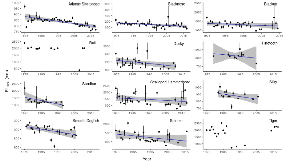
Survey results indicated > 9% relative decreases in L90% for all 10 species for which linear regression models were run (relative changes based on absolute trendlines; Figure 2.1). The largest relative declines were seen in sandbar shark (35%; 541 mm) and spinner shark (28%; 399 mm) (Table 2.1). We found the strongest statistical support (p < 0.04) for L90% declines in four species: blacknose shark (10%; 115 mm), dusky shark (23%; 297 mm), smooth dogfish (17%; 178 mm), and Atlantic sharpnose shark (10%; 88 mm) (Table 2.1). Using a conservative
43
Patterns in mean FL over time followed similar overall trends: 10 of 12 species were characterized by FLs that trended over time toward smaller average sizes (Figure 2.2).
Exceptions included tiger shark and bull shark. Tiger shark were defined by the almost complete absence of catches from 1990 through 2010 – with the exception of three small (< 1000 mm FL) individuals – bracketed by the occurrence of relatively large individuals (1500-2500 mm FL) in the survey during the 1970’s-1980s and 2010s (Figure 2.2). Except for one small (390 mm FL) bull shark captured in 2008, which had significant leverage in the regression analysis, individuals routinely measured ~2000 mm FL throughout the survey. Using trendline patterns among species other than tiger shark and bull shark, the largest relative decline in mean FL was observed for sandbar shark (20%; 214 mm), while the range of declines across all other species was 2-17% (Table 2.1). The strongest statistical support (p = 0.001) for a mean FL decline was found in blacknose shark, which declined by 11% (116 mm) (Table 2.1). Blacknose shark was also the only species characterized by a potential decline (4%; 41 mm) in mean FL using a relatively conservative approach (Table 2.1). Using a “worst-case scenario”, mean FL declined 12-55% across 10 species (largest decline for sandbar shark), with average sizes potentially shrinking by > 32% in seven of those species (Table 2.1).
44
declines in median FL ranged from 13-51% in a “worst-case scenario” among species other than spinner shark, tiger shark, or bull shark. As with mean FL, largest potential declines in median Fl were suggested for sandbar shark, with four species expressing > 31% reductions in median FL over time (Table 2.1).
Several sharks exhibited obvious reductions in catches of individuals within the largest size class of that particular species through time, including blacknose shark, silky shark, blacktip shark, sandbar shark, smooth dogfish and scalloped hammerhead (Figure 2.4). Across these species, the loss of largest individuals was generally evident sometime during the 1990s, mirroring declines in overall CPUEs for those species over the same period. Atlantic sharpnose shark was also characterized by the loss of the largest size class (800-1000 mm FL) by the end of the survey period, but with a couple of important nuances. (1) Catches of 800-1000-mm FL individuals appeared highest in the years between 1980-2005, whereas for other species, highest catches of the largest size class tended to occur between 1975-1995. And (2) Atlantic sharpnose shark was the only species that showed an increasing trend in annual mean CPUE (all size classes combined), from one shark per 100 hooks in the 1970s to seven sharks per 100 hooks by the 2000s (Figure 2.4).
Discussion
45
shark, spinner shark, tiger shark), Small Coastal Shark complex (Atlantic sharpnose shark, finetooth shark), Hammerhead Shark complex (scalloped hammerhead), Smoothhound complex (smooth dogfish), Harvest-Prohibited complex (dusky shark), Research-Only-Harvest species (sandbar shark) and individually managed species (blacknose shark). Below, we consider how observed decreases in sizes across species fit in the context of management, genetic versus environmental drivers of size structure within fished populations, and purported “mesopredator release.”
We readily acknowledge that the nature of this long-term, two-station, observational dataset presents some logistical challenges for applying standard statistical approaches to assess changes in size structure among species. We have attempted to respect these constraints by evaluating multiple metrics of size structure for thoroughness, as well as using a ‘totality of evidence’ approach regarding size trends, confidence intervals, and statistical clarity to draw ecological inferences. We also conclude that there is important meaning at the assemblage level in the consistency of trends across species over decadal time scales. Across all 12 species for which we evaluated mean and median sizes (and all 10 species assessed using L90%), we recorded
decreasing sizes through time based on the raw sign of fitted slopes. The probability of recording consistently negative slopes across 12 species – presuming size-structure was actually stable across species (i.e., a coin flip between the raw sign of slope being positive versus negative for each species [excluding zero slope]) – is only < 0.05% (< 1-in-4,000). Therefore, we conclude that the interpretation of across-assemblage decreases in sizes is likely robust.
46
significant contributor to both the size and catch patterns we observed. At the assemblage level, commercial landings for sharks included in this study in the NOAA Fisheries South Atlantic region rose during the 1970s- 1980s to a peak of 4,324 metric tons in 1994 (NOAA 2019). Since that peak, landings have declined by ten-fold at the assemblage level, with similar declines in harvest for many species. Exceptions include blacknose shark and blacktip shark, which showed modest increases in landings, as well as Atlantic sharpnose shark, for which the pattern was reversed (landings increased by ten-fold). These recent, lower landings are presumed to result from harvest-induced reductions in shark abundances as well as reductions in allowable catches (Final Consolidated Atlantic Highly Migratory Species Fishery Management Plan; NMFS 2006). Notably, the mid-1990s peak in catches, and rapid decline in landings since, corresponds to the loss of the largest size classes of blacknose shark, silky shark, blacktip shark, sandbar shark, smooth dogfish, and scalloped hammerhead (Figure 2.4).
While there is compelling evidence that tighter harvest management over the last two
47
Across management units, the consistent patterns of size decreases among species may also suggest something about mechanisms by which fishing impacts size structure. Shark
management complexes generally operate without minimum size limits, thereby reducing the potential for this to drive size-selective fishing. Therefore, perhaps coastal shark population size shifts could be driven by the selectivity of fishing gear (Stevens et al. 2000), which often target larger individuals. Furthermore, recreational fisheries for Large Coastal Sharks and Hammerhead Shark complexes do operate with minimum size requirements, while commercial fisheries for “ridgeback” Large Coastal Sharks operated with a minimum size from 1999-2003 (NMFS 2006). If minimum size regulations were a primary driver of reductions in mean body size, it makes little sense that species within these management units would be showing the most notable signs of potential increase over the last few survey years. Finally, the lack of recovery in either catch rates or sizes of sandbar shark since the mid-1990s, despite its status as a research-only-harvest species, invokes several possibilities: (1) the life-history of this species does not allow recovery under current, presumably modest, rates of research harvest; (2) environmental conditions have shifted and do not support rapid recovery of this species; and (3) the life history of this species does not allow recovery under current, poorly quantified, rates of non-target bycatch mortality (Crowder and Murawski 1998).
Regarding the dynamics of genetic versus environmental drivers of size structure within fished populations, our data indicate, at a minimum, that compensatory processes within the life history of sharks do not appear broadly capable of completely counteracting the effects of fishing on population size structure (Stevens et al. 2000). This, however, does not preclude the
48
context – simply reversed – Atlantic sharpnose shark was the lone species in our survey defined by increases in catch rates over time. Carlson and Baremore (2003) reported that Atlantic sharpnose shark exhibited increased juvenile growth rates in response to population declines, suggesting this may be a mechanism for density-dependent regulation. Thus, higher intraspecific competition for resources (i.e., lower growth rates) rather than just fishing pressure, could explain some of the decreases in sizes we observed for Atlantic sharpnose shark (sensu Cushing 1995).
While the assemblage-level decreases in size we observed may simply reflect the long-term press of continually removing the large(r) individuals from the stock, the opportunity for selective forces to impact shark populations and potential shark recovery appears present (Walker 1998). We are unable to arbitrate between these different and potentially co-occurring mechanisms within our analyses. Rather, the results presented here represent an important first step by documenting size-based indicators over appropriate timescales (i.e., years to decades), which should guide further exploration into the dynamics and root mechanisms of size-structure shifts. Despite the logistic challenges of examining sharks in the context of Darwinian fisheries (e.g., generation times of sharks, handling sharks for controlled experiments), we suggest this is an important area of investigation given the particular life histories and management approaches within this guild.
Size decreases reported in this study represent possible changes in recruitment, given
49
at parturition was the larval trait that most highly correlated with larval performance in black rockfish, with larvae from cohorts with the largest oil globules displaying a three-fold increase in growth rate and two-fold increase in survival rate (Berkeley et al. 2004). Maternal provisioning in sharks appears to occur via enlarged livers of offspring, with neonatal carcharhinid sharks showing a declining trend in liver mass (as well as overall body mass) shortly after parturition, presumably the excess liver reserves provide a maternal head-start for offspring to use in the first weeks of life (Hussey et al. 2010). Hussey et al. (2010) also found a clear relationship between pup mass and maternal size, with mean pup mass increasing with maternal size, although there was evidence for a decline at the largest mother lengths.
50
For all four of these species, long-term trends suggest decreases in size, which runs counter to the notion of top-down “release.” Combined with the long-term declines in catch rates of blacknose shark and smooth dogfish, these results suggest that mesopredators also experience population responses to (“top-down”) fishing pressure. Indeed, Blacknose shark exhibited perhaps the clearest shift over time, with all of the indices examined showing declines of ~10% throughout the survey period with high statistical confidence (Table 2.1), as well as relatively lower proportions of larger size classes in later years of the survey (Figure 2.4).
This study provides a baseline for future coastal shark size structure comparison, while also serving as a critical step for considering how shark populations may have responded to fishing via environmental versus genetic mechanisms. Over the next few decades, there is perhaps a unique opportunity to monitor size structure in populations of coastal sharks in the Fisheries Southeast regional as managers attempt to reverse past overharvest (Peterson et al. 2017). As in other fishery stocks, size structure is a critical component of monitoring and an indicator of stock health and resilience in the context of harvest pressure (Berkeley et al. 2004) and other,
51
REFERENCES
Allendorf, F. W., and J. J. Hard. 2009. Human-induced evolution caused by unnatural selection through harvest of wild animals. Proceedings of the National Academy of Sciences 106(Supplement 1):9987–9994.
Amrhein, V., F. Korner-Nievergelt, and T. Roth. 2017. The earth is flat (p > 0.05): significance thresholds and the crisis of unreplicable research. PeerJ 5:e3544.
ASMFC. 2008. Interstate fishery management plan for Atlantic coastal sharks. Atlantic States Marine Fisheries Commission, Washington, D.C.
Baremore, I. E., and M. S. Passerotti. 2013. Reproduction of the blacktip shark in the Gulf of Mexico. Marine and Coastal Fisheries 5(1):127–138.
Berkeley, S. A., C. Chapman, and S. M. Sogard. 2004. Maternal age as a determinant of larval growth and survival in a marine fish, Sebastes melanops. Ecology 85(5):1258–1264. Beverton, R. J. H., and S. J. Holt. 1957. On the dynamics of exploited fish stocks. Fisheries
Investigations Series 2(19). Ministry of Agriculture, Fisheries and Food, London, U.K. Birkeland, C., and P. K. Dayton. 2005. The importance in fishery management of leaving the big
ones. Trends in Ecology & Evolution 20(7):356–358.
Brashares, J., L. Prugh, C. J. Stoner, and C. Epps. 2010. Ecological and conservation
implications of mesopredator release. Pages 221–240 in John Terborgh and J. A. Estes, editors. Trophic Cascades: Predators, Prey, and the Changing Dynamics of Nature. Island Press, Washington, D.C.
Carlson, J. K., and I. E. Baremore. 2003. Changes in biological parameters of Atlantic sharpnose shark Rhizoprionodon terraenovae in the Gulf of Mexico: evidence for density-dependent growth and maturity? Marine and Freshwater Research 54(3):227.
Conover, D. O., and S. B. Munch. 2002. Sustaining fisheries yields over evolutionary time scales. Science 297(5578):94–96.