A TWO-DIMENSIONAL DIRAC SYSTEM AND ENVELOPE SOLUTIONS TO THE NONLINEAR SCHR ¨ODINGER EQUATION
David C. Webb
A dissertation submitted to the faculty of the University of North Carolina at Chapel Hill in partial fulfillment of the requirements for the degree of Doctor of Philosophy in the Department
of Mathematics.
Chapel Hill 2017
ABSTRACT
DAVID C. WEBB: A Two-Dimensional Dirac System and Envelope Solutions to the Nonlinear Schr¨odinger Equation
(Under the direction of Jeremy Marzuola)
In studying the cubic nonlinear Schr¨odinger (NLS) equation with hexagonal lattice potential, Ablowitz, Nixon, and Zhu [1] and Fefferman and Weinstein [31] have used ansatz solutions of a periodic, cubic NLS equation to derive two similar two-dimensional Dirac equations with cubic nonlinearity.
Chapters 1 and 2 of this thesis deal with solutions and lifespans of solutions for the linear and nonlinear Dirac equations. We establish local and almost global existence results as well as ill-posedness below the critical regularity, ˙H1/2. We leave as an open question whether solutions blow up in finite time or if a global existence result can be found.
The third chapter modifies the machinery of [32] and [31] to explore an open question posed by Fefferman and Weinstein, [31]. We prove that an envelope of solutions to the slowly modulated Dirac equation provides a good approximation for solutions to the nonlinear Schr¨odinger equation with hexagonal lattice. The NLS solution is shown to exist for long times with the nonlinear Dirac dynamics affecting the solution on any constant timescale. The same timescale is also proven for an ansatz envelope proposed by Ablowitz, Nixon, and Zhu. The timescale is also extended in an intermediate regime by slightly weakening the nonlinearity of the governing Dirac equation.
ACKNOWLEDGEMENTS
TABLE OF CONTENTS
LIST OF FIGURES . . . viii
Chapter 0. Introduction . . . 1
0.1. Motivation for the Equation . . . 2
0.2. Background . . . 4
1. Linear Results . . . 6
1.1. Basic Results . . . 6
1.1.1. Solution Operator . . . 6
1.1.2. Global Well-Posedness . . . 7
1.2. Analytic Support of Numerical and Experimental Observations . . . 10
1.2.1. Gaussian Initial Data . . . 10
1.2.2. Decay Away from the Light Cone . . . 12
1.2.3. Finite Propagation Speed . . . 14
1.3. Strichartz Estimates . . . 15
1.3.1. Statement of Desired Strichartz Estimate . . . 16
1.3.2. Proving the Strichartz Estimates . . . 18
1.3.3. Extending to r=∞ . . . 23
1.3.4. Conclusion of Strichartz Estimates . . . 24
2. Nonlinear Results . . . 26
2.1. Remarks on Conservation Laws, Scaling, and Criticality . . . 26
2.1.1. Nonlinear Conservation Laws . . . 26
2.2. Local Existence . . . 30
2.2.1. An Energy Existence Result . . . 31
2.2.2. Improvement Using Bootstrap Space . . . 35
2.3. Almost Global Existence . . . 38
2.3.1. The Vector Fields . . . 39
2.3.2. Almost Global Existence . . . 41
2.4. Ill-Posedness Below ˙H12 . . . 45
2.4.1. Choice of Initial Data . . . 45
2.4.2. Establishing a Lower Bound . . . 46
2.4.3. The Contradiction . . . 48
2.4.4. Extending to Another Nonlinearity . . . 48
2.5. Discussion of Global Existence Versus Blow-Up . . . 50
2.5.1. Lack of the Null Form . . . 50
2.5.2. Resonances of the Equation . . . 53
2.5.3. Blowup in the Quadratic Three-Dimensional Dirac Equation . . . 56
3. Application to the Schr¨odinger Ansatz . . . 58
3.1. Survey of the Relevant Floquet-Bloch Theory . . . 59
3.2. Further Preliminaries . . . 62
3.3. Beginning the Proof . . . 67
3.4. Bounding the η Independent Terms . . . 69
3.4.1. Estimation ofkfI,D(·, t) +α⊥I,D(·, t)kL2( R2) . . . 71
3.4.2. Estimation ofkfII,D(·, t) +α⊥II,D(·, t)kL2( R2) . . . 77
3.4.3. Estimation ofkfDc(·, t) +α⊥Dc(·, t)kH2( R2) . . . 79
3.4.4. Estimating theβ term,A2 . . . 82
3.4.5. Estimation ofkgDc(·, t)kH2( R2) . . . 85
3.5.1. EstimatingkA3,n+1(·, t)kH2(
R2) . . . 86
3.5.2. EstimatingkA4,n+1(·, t)kH2( R2) . . . 87
3.5.3. EstimatingkA5,n+1(·, t)kH2( R2) . . . 87
3.6. Bootstrapping η to Existence . . . 88
3.7. Weakening the Nonlinearity . . . 92
3.7.1. Finding the Corresponding Bounds . . . 95
3.7.2. Bootstrapping η to a Longer Timescale . . . 99
3.7.3. Why Does the Linear Dirac Not Suffice? . . . 101
3.8. Tight Binding Regime . . . 103
3.8.1. Finding the Corresponding Bounds . . . 107
3.8.2. Bootstrapping . . . 110
4. Numerical Simulations and Future Work . . . 111
4.1. Strang Splitting Methods . . . 111
4.1.1. Introduction and Theory . . . 111
4.2. Numerical Results . . . 114
4.2.1. Dispersion Surfaces . . . 114
4.2.2. Dirac Experiments . . . 115
4.2.3. Schr¨odinger Experiments . . . 118
4.2.4. Tight Binding Small Data . . . 119
4.2.5. Tight Binding Large Data . . . 120
4.2.6. Non-Tight Binding Small Data . . . 120
4.3. Conclusions and Future Work . . . 121
4.3.1. Future Work . . . 122
LIST OF FIGURES
4.1. Plots of dispersion surfaces . . . 115
4.3. Evolution of the Dirac equation . . . 116
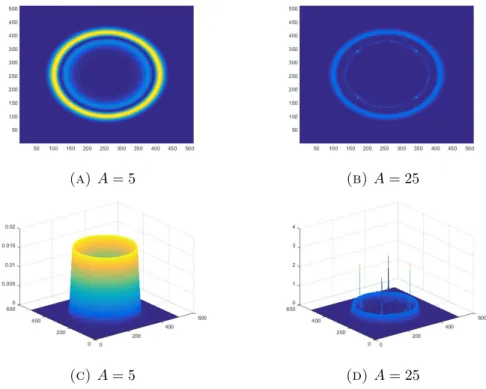
4.5. The effect of larger initial data on the simulation . . . 117
4.7. Effects of larger, double-Gaussian initial data . . . 118
4.8. Small data, tight binding NLS evolution . . . 119
4.10. Large data, tight binding NLS evolution . . . 120
CHAPTER 0
Introduction
The majority of this dissertation will be given over to studying the behavior of solutions to a particular two-dimensional system of Dirac equations with a cubic nonlinearity,
i∂tu−(∂x−i∂y)v=|u|2u i∂tv+(∂x+i∂y)u=|v|2v (0.1)
with initial data u(0,x) = f(x), v(0,x) = g(x). We will denote U =
u v
a solution to the equation. This equation will be written in several alternate forms throughout this dissertation. The most common will be by defining the differential operatorP as follows:
(0.2) P
u v
=
i∂t −∂x+i∂y ∂x+i∂y i∂t
u v
=
|u|2u |v|2v
.
We also will define the function F. When studying the linear equation, F will merely be the inhomogeneity
F(t, x, y) =
F1(t, x, y)
F2(t, x, y)
. When studying the nonlinear equation F will be the nonlinearity
F(u, v) =
|u|2u |v|2v
.
Thus the Dirac system can be written in the condensed formP U =F. To get another way we will represent the equation we define the operator
˜ P =
i∂t ∂x−i∂y
−∂x−i∂y i∂t
This operator is important because ˜P P =−2Id where 2 is the wave equation operator. Thus we can act on the Dirac equation by ˜P to get
−2u
−2v
=
i∂t ∂x−i∂y
−∂x−i∂y i∂t
F1
F2
=
i∂tF1+∂xF2−i∂yF2
i∂tF2−∂xF1−i∂yF1
(0.3)
with initial data U(0,x) =
f(x) g(x)
and Ut(0,x) =
−i|f|2f −ig
x−gy
−i|g|2g+if
x−fy
.
Thus solutions to the Dirac equation will also solve the above wave equation. We will see later that the fundamental solution operator to the Dirac equation has many similarities to the wave equation solution operator. Considering both of these facts, the large body of research in wave equations becomes immediately useful.
We will also work with the similar Dirac equation derived in [31] by Fefferman and Weinstein: ∂tu+λ# ∂x+i∂y
v=−ig β1|u|2+ 2β2|v|2
u ∂tv+λ# ∂x−i∂y
u=−ig 2β2|u|2+β1|v|2
v (0.4)
whereλ#,βj, andgare constants defined in [31]. Throughout Chapters 1 and 2 we work primarily
with (0.1) as it will be easier to deal with notationally. However, the arguments will apply identically to (0.4). In Chapter 3 we will work more closely with Equation 0.4 as it works more readily with the machinery used in that chapter.
0.1. Motivation for the Equation. The above Dirac equation is derived from optical physics in Ablowitz, Nixon, Zhu [1] as well as in Ablowitz, Zhu [2]. They are studying the behavior of light passing through the material optical graphene, which is an optical material with a hexagonal lattice. In particular they are studying what happens when the wavelength of light used corresponds to certain coordinates (called diabolical points) of the lattice.
They begin by using the nonlinear Schr¨odinger (NLS) equation,
(0.5) iΨt+ ∆Ψ−V(x)Ψ +σ|Ψ|2Ψ = 0,
whereb1= (0,1),b2= (−
√
3 2 ,−
1
2),b3 = (
√
3 2 ,−
1
2) represent the nearest neighbors to any particular
node on the lattice.
Ablowitz, Nixon, and Zhu [1] create an ansatz for the NLS for which solutions to the Dirac system serve as an appropriate envelope within the ansatz, (0.1). However, it is important to note that their derivation of the Dirac system is not mathematically rigorous. It is a reasonable guess for a model to describe a behavior of optical graphene. Part of our exploration of this Dirac system will be to determine how well this model matches the experimental and numerical data as well as investigating on what time scales the model may be a good fit.
In [1] the authors ran numerical simulations inputting Gaussian initial data into the Schr¨odinger equation. In their simulations there appear to be 3 major qualities we see in the solution. While the solutions do not appear to be perfectly rotationally invariant, it does seem that|Ψ(r, θ1)| ∼ |Ψ(r, θ2)|
for any choice of θi. In other words, r appears to have a much greater impact on the size of the solution than does θ. Also, the solution appears to decay as you move away from the light cone. Most interesting is the fact that for their choice of initial data it appears that the solution has finite speed of propagation. This last result is quite notable as the Schr¨odinger equation is known to have infinite propagation speed.
The authors also ran numerical simulations for the derived linear Dirac system. In one of these simulations they input initial data that is Gaussian in one coordinate and zero in the other. This result also shows decay away from the light cone and finite speed of propagation. However, it also appears that |U| is perfectly rotationally invariant showing some variance from the Schr¨odinger model. In another simulation, both components of the initial data were Gaussian. In this case, the decay off the light cone and finite propagation speed still appear, but the rotational invariance has disappeared completely. Not all of these numerical results are particularly notable. However, we include them here as we will analyticaly confirm these observations in Chapter 1.
In the nonlinear section we will consider several function spaces and determine on what time scale solutions to the Dirac equation will exist in those spaces.
The Dirac equation derived by Fefferman and Weinstein, (0.4), is found by working with an ansatz solution to the periodic potential Schr¨odinger equation (0.5). They scale unknown functions u and vby a small constant, δ, and show that the error term in the ansatz can be held small on a large timescale ifu and v are components of the solution to the Dirac equation (0.4).
Their choice of ansatz is motivated by their work in [32] in which they prove a similar result for the corresponding linear Schr¨odinger and Dirac equations. Their work in [31] poses an open question using the solutions to (0.4) as ansatz envelopes for solutions to the NLS equation. They discuss some of the key changes and steps of the proof, but they do not actually provide a full proof for the ansatz solution nor do they give a timescale for the ansatz. In Chapter 3, we will modify the ansatz proposed by Fefferman and Weinstein and prove a timescale for which the ansatz solutions hold. We will also adapt the argument to an ansatz proposed by Ablowitz and Zhu, [2], which is more complicated because of different time and space scalings in their ansatz and certain assumptions they make, in particular that the potential is tight binding.
0.2. Background. As we have already shown that results pertaining to the wave equation are relevant to the Dirac equation in question we will begin by looking at established results for the wave equation particularly with cubic nonlinearity in two dimensions.
The case of the cubic wave equation in two dimensions is quite interesting. Li, Zhou showed in [78] that small data global solutions exist for all nonlinearities of power greater than three. Also, there are several examples, [3], [57] , [84] of cubic nonlinearities that result in nonexistence of global solutions even in small data. For a general cubic nonlinearity the existence time has only been shown to have a lower bound T∗ ≥c−6 with the size of the initial data, [77].
Almost global results have been obtained whererepresents the size of the initial data. Kovalyov [54] proved a timescale of T∗ ≥ exp (c−2) for a class of nonlinearities that only depend on first and second derivatives of the solution. Li, Zhou [77] proved the same timescale by assuming ∂u3F(0,0,0) =∂u4F(0,0,0) = 0 where F(u, Du, DxDu) is the nonlinearity. Katayama [47] dropped the assumption ∂u4F(0,0,0) = 0 and proved the timescale T∗ ≥ −18. However, he also proved another almost global result for when the nonlinearity satisfies an almost-null condition.
a null condition, and Katayama, [46] proved the same when only assuming the cubic part of the nonlinearity satisfies a null condition. In [48] Katayama proved a small data global result for a weaker null condition analagous to that of Alinhac [6] for three dimensions. Hoshiga [40] was able to prove a small data global existence result for a class of nonlinearity that does not satisfy a null condition. Also important to mention is the work of Alinhac [5] where he proves small data global existence for a large class of cubic derivative nonlinearities which satisfy two null conditions.
In general there is not as much literature studying the Dirac equation (massive or massless), and only a small amount of that literature deals with the two-dimensional case. In the one-dimensional case Pelinovsky [67] was able to prove small data global existence in H1 for the massive Dirac equation with cubic nonlinearity. His proof relies on conservation laws for the equation and shows that a time dependent upper bound for the equation may continually grow but always remains finite.
In the three-dimensional case Escobedo and Vega [27] prove local well-posedness for the massive cubic Dirac equation in H1+. This result was extended to small data global well-posedness by Machihara, Nakanishi, and Ozawa, [62], in the same space. Machihara, Nakamura, Nakanishi, and Ozawa, [61], were able to improve the regularity of the global result to H1. Also in three dimensions Bejenaru and Herr [16] proved a small data global result for the massive equation with a different cubic nonlinearity in the space H1 relying on the endpoint Strichartz estimates for the Klein-Gordon equation.
In the two-dimensional case Pecher [66] was able to show local well-posedness in H12+ for a
massive Dirac equation with a nonlinearity satisfying a null form. In a recent article Bejenaru and Herr [17] have improved this to small data global existence for the critical spaceH12 by once again
using the endpoint Strichartz estimates for the Klein-Gordon equation. Bournaveas and Candy [20] have been able to prove a similar small data global result in ˙H12 for a cubic, massless equation
CHAPTER 1
Linear Results
1.1. Basic Results.
1.1.1. Solution Operator. Before we can move on to more interesting results, we need to first establish the solution operator of the Dirac equation. This will be found by applying the Fourier Transform to the equation, diagonalizing the resulting operator, exponentiating the diagonalized operator, reverting to the undiagonalized form, and applying the Inverse Fourier Transform. As the title of this sections implies, the results of this section are very basic. Because everything in this paper relies on these basic results, we cover this initial section in great detail in the interest of thoroughness.
By applying the Fourier Transform to the homogeneous equation, we get i∂tuˆ−(iξ1+ξ2)ˆv= 0
i∂tˆv+(iξ1−ξ2)ˆu= 0.
(1.1)
Definingz=ξ2+iξ1 We can rewrite this as
(1.2) i∂t
ˆ u ˆ v
=
0 z ¯ z 0
ˆ u ˆ v
:= ˆH
ˆ u ˆ v
.
Notice that to do this we have assumed z 6= 0. In the case z = 0 we also have ξ = 0 and the equation reduces to an ordinary differential equation with solutionU = (f, g) which is what we get if we replace ξ= 0 in the solution operator we find below.
Now we can find the solution operator in Fourier Space, eitHˆ, by diagonalizing ˆH. We find eigenvectors of ˆH to bep1 =
z
|z|
andp2=
z
−|z|
.Thus to diagonalize ˆHwe conjugate it by
(1.3) A=
z z
|z| −|z|
Thus
DHˆ =A−1HˆA
=
|z| 0 0 −|z|
. (1.4)
Now, since DHˆ is a diagonal matrix, it is easy to compute
(1.5) e−itDHˆ =
e−it|z| 0 0 eit|z|
.
Then conjugating backwards results in
e−itHˆ =Ae−itDHˆA−1
=
cos(t|z|) |izz|sin(t|z|) iz¯
|z|sin(t|z|) cos(t|z|)
. (1.6)
Thus we have the solution operator ˆ u ˆ v
= e−it
ˆ H ˆ f ˆ g
. By applying the inverse Fourier Transform we find
u v
=F −1
cos(t|z|) ˆf+|izz|sin(t|z|)ˆg iz¯
|z|sin(t|z|) ˆf+ cos(t|z|)ˆg
. (1.7)
Then noting that|z|=|ξ|we substitute into the above equation giving the solution operator
(1.8) u v
=F −1
cos(t|ξ|) ˆf+ −ξ1+iξ2
|ξ| sin(t|ξ|)ˆg
ξ1+iξ2
|ξ| sin(t|ξ|) ˆf
+ cos(t|ξ|)ˆg
.
1.1.2. Global Well-Posedness. In this section we will prove global well-posedness for the in-homogeneous linear equation. Having already found the solution operator for the in-homogeneous equation we will use Duhamel’s principle to find the solution to the inhomogeneous equation. Then we will express an upper bound of the Sobolev norm of this solution in terms of the Sobolev norms of the initial conditionsf, gand the inhomogeneitiesF1, F2.Global well-posedness will easily follow
1.1.2.1. Solving the inhomogeneous equation. The solution of the homogeneous equation has been found to be
(1.9) U =
u v
=F −1
cos(t|ξ|) ˆf+ −ξ1+iξ2
|ξ| sin(t|ξ|)ˆg ξ1+iξ2
|ξ| sin(t|ξ|) ˆf + cos(t|ξ|)ˆg
.
Duhamel’s principle tells us that the solution to the inhomogeneous case with zero initial con-ditions is in fact an integral of the solution to the homogeneous case with initial concon-ditions equal to the original inhomogeneity. In other words, the solution to
i∂tu−(∂x−i∂y)v =F1(t, x, y)
i∂tv+(∂x+i∂y)u=F2(t, x, y)
(1.10)
withu(0, x, y) =v(0, x, y) = 0 is given by
(1.11) u v
=−i Z t
0 F−1
cos[(t−τ)|ξ|] ˆF1(τ, ξ) +−ξ1|ξ+|iξ2sin[(t−τ)|ξ|] ˆF2(τ, ξ)
ξ1+iξ2
|ξ| sin[(t−τ)|ξ|] ˆF1(τ, ξ) + cos[(t−τ)|ξ|] ˆF2(τ, ξ)
dτ.
The solution for the inhomogeneous equation with nonzero initial data is merely the sum of the solutions to the two above cases:
U = u v
=F−1
cos(t|ξ|) ˆf +−ξ1+iξ2
|ξ| sin(t|ξ|)ˆg ξ1+iξ2
|ξ| sin(t|ξ|) ˆf + cos(t|ξ|)ˆg
+F−1
−iR0t cos[(t−τ)|ξ|] ˆF1(τ) +−ξ1|ξ+|iξ2 sin[(t−τ)|ξ|] ˆF2(τ)
dτ
−iRt
0
ξ1+iξ2
|ξ| sin[(t−τ)|ξ|] ˆF1(τ) + cos[(t−τ)|ξ|] ˆF2(τ)
dτ
. (1.12)
1.1.2.2. Bounding the Solution. Assume that f, g ∈ S and F1, F2 ∈ C∞([0,∞],S). Then we can
drop the inverse Fourier transform inside the L2 norm without changing the value. Then, by applying the triangle inequality we can see that
kukL2 ≤
cos(t|ξ|) ˆf L2 +
−ξ1+iξ2
|ξ| sin(t|ξ|)ˆg
L2 + Z t 0
cos[(t−τ)|ξ|] ˆF1(τ, ξ)
L2+
−ξ1+iξ2
|ξ| sin[(t−τ)|ξ|] ˆF2(τ, ξ)
L2dτ.
(1.13)
Then we note that |cos(t|ξ|)|,|sin(t|ξ|)|,|−ξ1+iξ2
|ξ| | ≤1,and the above immediately becomes (1.14) kukL2 ≤ kfˆkL2 +kgˆkL2+
Z t
0
Fˆ1(τ,·)
L2 +
Fˆ2(τ,·)
L2
Once again since in Schwartz space the L2 norm of a function is the same as the L2 norm of its Fourier transform, this becomes
(1.15) kukL2 ≤ kfkL2+kgkL2 +
Z t
0
F1(τ,·)
L2 +
F2(τ,·)
L2
dτ.
The exact same bound is found for kvkL2 with the same procedure leading to the bounds
kUkL2 ≤C
kfkL2+kgkL2+
Z t
0
(kF1(τ)kL2 +kF2(τ)kL2)dτ
kUkHs ≤C
kfkHs +kgkHs+
Z t
0
(kF1(τ)kHs+kF2(τ)kHs)dτ
(1.16)
where the Hs norms are possibly infinite because we have not assumed initial data and inhomo-geneities in the appropriate spaces.
1.1.2.3. Global Well-Posedness in Hs. Now assume that f, g ∈ Hs and F1, F2 ∈ L1([0,∞], Hs).
Because of the density ofS inHs we can choose sequences fj, gj ∈ S andF1,j, F2,j∈L1([0,∞],S) such that asj → ∞each converges to its obvious limit. In other words,
kfj−fkHs →0, kgj−gkHs →0, kF1,j−F1kHs →0, kF2,j−F2kHs →0.
We will denote Uj to be the corresponding solutions to the Dirac equation with initial data fj, gj and inhomogeneity F1,j, F2,j.Then the work we have done for Schwarz initial data gives us
(1.17) kUj −UkkHs .kfj−fkkHs+kgj−gkkHs +
Z t
0
kF1,j−F1,kkHs +kF2,j−F2,kkHsdτ.
Thus the sequence Uj is Cauchy in the Banach Space Hs, and hence converges to some U. But Uj → U in the distributional sense as well. Thus P Uj →P U where P is our differential operator. But
(1.18) P Uj =
F1,j F2,j
→
F1
F2
.
ThusP U =
F1
F2
Since the bound forkUjkHs holds for everyj, the same bound holds for the limit,kUkHs.Thus
we have
kUkHs ≤C
kfkHs +kgkHs+
Z t
0
(kF1(τ)kHs+kF2(τ)kHs)dτ
≤CkfkHs +kgkHs+kF1(τ)kL1
tHxs +kF2(τ)kL1tHxs (1.19)
forf, g∈Hs andF1, F2∈L1([0,∞], Hs).
Since f, g∈Hs and F1, F2∈L1([0,∞], Hs),Inequality (1.19) immediately shows thatU ∈Hs
sincekUkHs has a uniform bound for all time.
For uniqueness since we are in the linear case it is sufficient to show that when f =g =F1 =
F2= 0 thenU must also be 0. This is trivial from (1.19).
To show that the solution depends continuously on initial data let us assumeU∗ is the solution for initial data f∗ and g∗ with the same inhomogeneity as the equation forU. Then
(1.20) kU−U∗kHs ≤C
kf−f∗kHs+kg−g∗kHs
which is the desired statement.
1.2. Analytic Support of Numerical and Experimental Observations. The purpose of this section is to support some of the qualitative observations made by the numerical work in [1]. The subsection on Gaussian initial data supports the radial symmetry seen in [1], but is not strictly applicable to the later work in this dissertation. The subsection establishing decay away from the light cone is interesting as it quantifies the Huygens-like behavior seen in [1], but, once again, we do not make further use of it. The finite speed of propagation is vital for several of the nonlinear results in Chapters 2 and 3.
1.2.1. Gaussian Initial Data. The experimental and numerical work done in [1] features radially symmetric initial data. Therefore we will analyze what happens when a Gaussian initial condition is input into the homogeneous linear Dirac equation. When discussing rotational invariance we will be working with the homogeneous Dirac equation
One important property of the Gaussian function that we will use regularly is that the Fourier transform of a Gaussian,e−k1|x|2, is a different Gaussian,e−k2|ξ|2. For the sake of simplicity we will
just normalize the coefficient k1 = 1, k2 =k.
1.2.1.1. The Magnitude of the Solution. We will now assume that f = e−|x|2 and g = 0. Then substituting in the initial conditions we find that
u(x, t) =F−1cos(t|ξ|)e−k|ξ|2
:=ψ1(x, t)
v(x, t) =(−i∂x+∂y)F−1
1
|ξ|sin(t|ξ|)e
−k|ξ|2
:=(−i∂x+∂y)ψ2(x, t).
(1.21)
Now we consider the absolute value of our solution,|U|=p|u|2+|v|2.Definingψ
1, ψ2as above
we notice that both are inverse Fourier transforms of even, real-valued functions and are thus real valued. Thus the real and imaginary parts of uand v are easy to calculate, and we find |u|2 =ψ2 1
and |v|2 =ψ2
2,x+ψ22,y. Thus
(1.22) |U|= (ψ12+ψ22,x+ψ22,y)1/2.
It is important to note thatψ2 was defined as the sine term of the solutionafter theξ1, ξ2 have
been pulled outside of the Inverse Fourier Transform as derivatives.
1.2.1.2. Rotational Invariance. Now we must stop and show that ψ1(x, t) and ψ2(x, t) are both
rotationally invariant.
In order to do this we will first convert both into polar coordinates. Then, by doing a carefully chosen change of variables we can eliminate the dependence on θ in the equations. Once there is no dependence onθ, it is trivial to say the function is rotationally invariant.
We first show this forψ1,
ψ1(x, t) =C
Z
eix·ξcos(t|ξ|)e−k|ξ|2dξ ψ1(r, θ, t) =C
Z
ei(rcos(θ)ξ1+rsin(θ)ξ2)cos(t|ξ|)e−k|ξ|2dξ
=C Z
ei[r(ξ1cosθ+ξ2sinθ)]cos(t|ξ|)e−k|ξ|2dξ.
Then we do a simple change of variables rotating ξ by −θ, η1 = ξ1cosθ +ξ2sinθ and η2 = −ξ1sinθ+ξ2cosθ. Thus |η|=|ξ|and dη=dξ.
ψ1(r, θ, t) =C
Z
eirη1cos(t|η|)e−k|η|2dη.
(1.24)
We can now see that ψ1 has no dependence on θ and is therefore rotationally invariant. Also we
can proceed similarly doing the same change of variables to show thatψ2 is rotationally invariant.
ψ2(x, t) =C
Z
eix·ξsin(t|ξ|)|ξ|−1e−k|ξ|2dξ ψ2(r, θ, t) =C
Z
ei(rcos(θ)ξ1+rsin(θ)ξ2)sin(t|ξ|)|ξ|−1e−k|ξ|2dξ
=C Z
ei[r(ξ1cosθ+ξ2sinθ)]sin(t|ξ|)|ξ|−1e−k|ξ|2dξ
=C Z
eirη1sin(t|η|)|η|−1e−k|η|2dη.
(1.25)
Here we now see that ψ2 is also rotationally invariant since it has no dependence onθ.
Now, we will rewrite (1.22) using the identityψ22,x+ψ22,y=ψ22,r+r12ψ22,θ.However, in our case
ψ2 is rotationally invariant, soψ2,θ = 0.Thus,|U|= q
ψ21+ψ22,r, and there is no dependence onθ. Thus we have confirmed that with the above Gaussian and zero initial conditions the solution to the linear Dirac problem maintains rotational invariance.
It is important to note that the above argument does not hold if the initial dataf, g are both Gaussian. In fact, if we assume that f and g are both Gaussian, then the above will verify that the solutions do not have radial symmetry, as indicated in the numerical work of [1].
1.2.2. Decay Away from the Light Cone. For the wave equation in odd spatial dimensions Huygens’ Principle holds stating that the value of the solution at a point (x, t) depends only on the values of the initial condition on∂B(x, t). In other words, solutions at a point are determined by the values of the initial data on a light cone centered at that point.
As we are working with a Dirac equation in 2 dimensions we do not expect this to hold. However, in the experimental and numerical work done in [1], the solutions appear to be concentrated near the light cone. In this section we analytically support that observation.
Lemma 1.2.1 (Klainerman-Sobolev Inequality).
(1.26) (1 +t+|x|)12(1 +t− |x| )
1
2|v(t,x)| ≤Ckv(t,·)k2,2
for any function v with finite right-hand side.
However, we need to define the norm on the right-hand side. To do this we introduce the following vector fields: Γ0 = t∂t+x∂x +y∂y,Ω01 = t∂x +x∂t,Ω02 = t∂y +y∂t,Ω12 = x∂y −
y∂x, ∂t, ∂x, ∂y. We index these vector fields by Γ = {Γi}6i=0.We discuss these more thoroughly in
the Almost Global section in Chapter 2. For now we just need to define
|v(t,x)|s= X
|α|≤s
|Γαv(t,x)|
kv(t,·)ks,p=|v(t,·)|s
Lp.
(1.27)
Using the Klainerman-Sobolev inequality, we can immediately state that for U, a solution to (0.1), we have
|U(t,x)| ≤(1 +t+|x|)−12(1 +t− |x| )−
1
2kU(t,·)k2,2
≤(1 +t− |x|
)−12kU(t,·)k2,2.
(1.28)
If the norm on the right-hand side is finite, then we see that there is decay away from the light cone. However, this statement is vacuous if the norm on the right-hand side is not finite.
For the linear, inhomogeneous Dirac equation it is a quick result that the norm on the right-hand side is finite. If U solves the linear, inhomogeneous Dirac equation, then U also solves the linear, inhomogeneous wave equation (0.3). As we mention more carefully in Section 2.3, each of these vector fields commutes well with the wave equation operator, 2, (except for Γ0 which gives
an extra copy of 2 when commuting with2). Thus,kU(t,·)k2,2 can be bounded:
(1.29) kU(t,·)k2,2≤C
kfk2,2+kgk2,2+
Z t
0
(kF1(τ)k2,2+kF2(τ)k2,2)dτ
.
As long as we restrict the initial data to be in the 2,2-norm space and the inhomogeneities to be L1 in time and be in the 2,2-norm space in space, then the right-hand side will stay finite. This analytically confirms the decay off the light cone seen in [1].
compactly supported. Thus for the nonlinear Dirac equation, we technically only prove decay off the light cone for small enough initial data with compact support (since that is when we are able to prove that the norm above is finite). However, Ablowitz, Nixon, and Zhu run their simulations for a short enough time scale (t= 10.8) that this gives us reasonable analytical support for the qualitative observations made in [1] even in the nonlinear case (in addition to confirming the observation for the linear case).
1.2.3. Finite Propagation Speed. In this section we will show that the Dirac equation has finite speed of propagation (FPS).
As we have already shown in the introduction, solutions to the Dirac equation also solve a particular wave equation. As it is well known that the wave equation has finite speed of propagation, this property easily transmits to the Dirac equation.
1.2.3.1. The Homogeneous Case. If we assumeU is a solution to the homogeneous Dirac equation, then we can simply apply the operator ˜P to the equation to conclude
(1.30)
−2u
−2v
=
−2 0 0 −2
u v
= ˜P P
u v
= ˜P ·0 = 0.
ThusU also solves the homogeneous wave equation.
Among many places, a proof for finite propagation speed of the wave equation is given in [28]. It states that ifusolves the wave equation andu=ut= 0 onB(x0, t0)× {t= 0}, thenu= 0 within
the backward light coneC={(x, t)|0≤t≤t0,|x−x0| ≤t0−t}.This is equivalent to saying that
if u0 is compactly supported on K, then for any time t > 0 we have that u(·, t) is supported on
B(K, t), all the points within a distance,t, from the support,K.
Thusu, vboth have finite propagation speed when they are solutions to the homogeneous Dirac problem.
Thus we are looking for a solution to
(1.31) P
u v
=
F1
F2
, u0 =v0 = 0.
Using Duhamel we first letu(x, t;τ) be a solution to
(1.32) P
u(x, t;τ) v(x, t;τ)
=
0 0
on R2×(τ,∞)
with initial conditions
(1.33)
u(x, t;τ) v(x, t;τ)
=
F1(x, t;τ)
F2(x, t;τ)
on R2× {t=τ}.
Then by Duhamel’s Formula the solution to (1.31) is merely u(x, t) = iR0tu(x, t;τ)dτ and similarly for v. This can be solved out further (which is done in the above section for Global Well-Posedness), but for the purposes of showing FPS this is all we need.
Notice that (1.32) is a homogeneous equation where the starting point is nowt=τ instead of t= 0. Thus F1(τ) having compact support on Kτ implies that u(x, t;τ) has compact support on B(Kτ, t−τ).
Now we will consider the case when F1(τ) has compact support, Kτ,for all τ.Then u(x, t) = iR0tu(x, t;τ)dτ is supported on the union of the balls, B(Kτ, t−τ).Notice that
∪tτ=0B(Kτ, t−τ)⊂B ∪tτ=0Kτ, t.
This yields FPS as long as ∪Kτ is bounded. However, this is trivial as it is just a union over a compact interval of compact sets. Notice also that v andF2(τ) are treated the same way.
In particular, forF1(τ) compactly supported onKτ for eachτ,We have thatu(x, t) is supported on B(∪t
τ=0Kτ, t),which is a bounded set.
We prove the following Strichartz estimates to allow us to get an improved local existence result for solutions to the nonlinear equation when working with Strichartz spaces. However, neither the Strichartz estimates nor the Strichartz space local existence result are needed in proving the main result in Chapter 3. Thus, these Strichartz estimates are mainly included for the sake of completeness and are found by making modifications to the wave equation Strichartz estimates.
It is also important to note that we will be reducing the solution operator to the half-wave operator. Thus, the Strichartz estimates are essentially the same as the well known Strichartz estimates for the wave equation with some modifications of the gap condition. Although originaly developed by Strichartz in [75], we will primarily make use of the proof in Lawrie, [56], to influence the overall strategy of the proof. In particular, his proof will work for the desired estimates with the addition of a Lemma from Stein, [73], and carefully tracking how the difference in the inho-mogeneous terms of the fundamental solution changes the gap condition. Also of use in motivating this section were Sogge, [72], and Selberg, [70]. Strichartz estimates for the wave equation were also proved in [35, 50, 51, 59].
We will work with the inhomogeneous Dirac equation i∂tu−(∂x−i∂y)v=n(t, x, y) i∂tv+(∂x+i∂y)u=m(t, x, y) (1.34)
with initial data u(0,·) =f(·) and v(0,·) =g(·) and inhomogeneities n andm.
1.3.1. Statement of Desired Strichartz Estimate. Before getting started we must discuss what particular mixed space-time norms will work for the Strichartz estimates. To do so we define the following:
Definition 1. We say that the pair (q, r) is wave admissible if
(1.35) 2≤q≤ ∞, 2≤r <∞ and 2 q ≤
n−1 2
1−2
r
.
In particular, since our Dirac equation is in 2 dimensions, wave admissible means
(1.36) 2
q ≤ 1 2−
We will assume that (q, r) and (˜q,r) are both wave admissible. We define˜ ST = [0, T]×R2. Then we claim the following Strichartz Estimates for the above Dirac equation:
Theorem 1.3.1. Let (q, r) be wave admissible. Assuming that U solves Equation 1.34 with
f, g∈H˙s(R2) andn=m= 0 (i.e. the homogeneous equation), then
(1.37) kUkLq
tLrx(ST) .kfkH˙s +kgkH˙s
where s, q, r satisfy 2r +1q = 1−s.
Notice that it suffices to prove this estimate foru (since the proof for v will be identical), and it is trivial to distribute using the triangle inequality and reduce to the half-wave operator
kukLq tLrx ≤
F
−1eit|ξ|fˆ
LqtLrx
+
F−1
−
ξ1+iξ2 |ξ| e
it|ξ|gˆ
LqtLrx
. (1.38)
We also state the desired Strichartz estimates for the inhomogeneous equation.
Theorem1.3.2. Let(q, r)and(˜q,r)˜ both be wave admissible. Assuming thatU solves Equation
1.34 with f, g∈H˙s(R2) and n, m∈Lq˜
0
t Lr˜
0
x(ST), then (1.39) kUkLq
tLrx(ST).kfkH˙s+kgkH˙s+knkLq˜0 t Lr˜
0
x(ST)+
kmk
Lqt˜0L˜r
0
x(ST)
where s, q, r,q,˜ ˜r satisfy the gap condition 2r +1q = 1−s= r˜20 +q˜10 −1.
Again, it suffices to prove this estimate foru (since the proof for v will be identical), and it is trivial to distribute using the triangle inequality and reduce to the half-wave operator
kukLq tLrx ≤
F
−1eit|ξ|fˆ LqtLr
x +
F−1
−
ξ1+iξ2 |ξ| e
it|ξ|gˆ
LqtLrx
+ Z t 0
F−1ei(t−τ)|ξ|n(τˆ )dτ
LqtLrx
+ Z t 0 F−1
−
ξ1+iξ2 |ξ| e
i(t−τ)|ξ|m(τˆ ) dτ
LqtLrx
. (1.40)
However, the proof for Theorem 1.3.1 will already establish the needed bounds for both homoge-neous terms. Thus, we only need to find bounds for the last two terms on the right-hand side of (1.40).
estimates and the Strichartz estimates for the wave equation. The other being using a lemma from [73] to deal with the −ξ1+iξ2
|ξ| multipliers in the second and fourth terms.
However, the gap condition in Theorem 1.3.2 along with wave admissability reduces to q = ˜
q = ∞ and r = ˜r = 2 which is just the L2 energy inequality for the equation. Thus, on its own, Theorem 1.3.2 is essentially trivial. We include it to show how the standard wave equation Strichartz arguments apply for the Dirac equation. We also include it so that we may introduce regularity on the right-hand side of the inequality (while using only minor modifications to the proof) to widen the condition governing the allowable pairs in the estimate. In order to do so we introduce the following theorem
Theorem1.3.3. Let(q, r)and(˜q,r)˜ both be wave admissible. Assuming thatU solves Equation
1.34 with f, g∈H˙s(R2) and n, m∈Lq˜
0
t Lr˜
0
x(ST), then (1.41) kUkLq
tLrx(ST).kfkH˙s +kgkH˙s+knk
L˜qt0W˙xs,˜r0(ST)+
kmk
Lqt˜0W˙xs,˜r0(ST)
and ssatisfies the condition 2r +1q = 1−s= r˜20 +q˜10 −1−s.
After the proofs, we will show that Theorem 1.3.3 can be extended to the near endpoint case q >4, r=∞ by appealing to a result of Fang and Wang, [29].
1.3.2. Proving the Strichartz Estimates.
1.3.2.1. Proof of Theorem 1.3.1. For the homogeneous estimates we rely entirely on the proof pro-vided in Lawrie, [56], with the addition of a minor modification to deal with the Fourier multiplier in the second term.
Lawrie uses the following pointwise estimate lemma
Lemma 1.3.4. Let f ∈ S be such that supp(ˆf)⊂ {12 ≤ |ξ| ≤2}. Then,
e
±it√−∆f
L∞
x
≤Chti−n−21kfkL1
e
±it√−∆f
L2 ≤ kfkL2.
(1.42)
Lawrie uses these estimates and the standardT T∗ argument to prove that
(1.43)
e
±it√−∆f
LqtLr x
for any f such that supp(ˆf)⊂ {1
2 ≤ |ξ| ≤2}. Using the restriction, 2
r+
1
q = 1−s, he then extends the inequality to the case where supp(ˆf)⊂ {2j−1 ≤ |ξ| ≤2j+1}.
He then extends the result to f without any assumption on the support of ˆf by using a Littlewood-Paley expansion
(1.44)
e
±it√−∆f
2
LqtLr x
≤X
j
kFjk2Lq tLrx
where Fj is e±it √
−∆f frequency localized on the diadic intervals {2j−1 ≤ |ξ| ≤ 2j+1}. In other
words,Fj = ˆψj∗e±it √
−∆f where{ψj}∞
j=1 is a diadic partition of unity. Since eachFj is frequency
localized on {2j−1≤ |ξ| ≤2j+1} he can apply (1.43) to get
(1.45)
e
±it√−∆f
2
LqtLrx
≤CX j
kψˆj∗fk2H˙s.
Using Littlewood-Paley theory again, he shows
(1.46) X
j
kψjˆ ∗fk2˙
Hs ≤ kfk
2 ˙ Hs and thus (1.47) e
±it√−∆f
LqtLrx
≤CkfkH˙s
giving the desired bound for the first term of (1.38).
To prove the desired bound for the second term of (1.38) we recognize that we can rewrite it as
(1.48)
e±it √
−∆
F−1−ξ1+iξ2 |ξ| ˆg
LqtLrx
.
Replacing f in (1.47) byF−1−ξ1+iξ2
|ξ| ˆgimmediately gives us (1.49)
e±it √
−∆
F−1−ξ1+iξ2 |ξ| gˆ
LqtLr x ≤C
F−1−ξ1+iξ2 |ξ| gˆ
˙ Hs .
Using the fact that
−ξ1+iξ2
|ξ|
= 1 and that the norm on the right-hand side is an L
2-based norm
we see that the norm on the right-hand side is equal tokgkH˙s. Thus we have the desired estimate
for the second term of (1.38)
(1.50)
e±it √
−∆
F−1−ξ1+iξ2 |ξ| ˆg
LqtLr x
This concludes the proof for Theorem 1.3.1.
1.3.2.2. Proof of Theorem 1.3.2. As mentioned after the statement of the theorem, the desired bounds for the first two terms of (1.40) are established by the proof for Theorem 1.3.1. Thus we only need to prove the desired bounds for the third and fourth terms of (1.40). We can rewrite the third term as
(1.51)
Z t
0
e±i(t−τ) √
−∆n(·, τ)dτ
LqtLr x
.
Looking back at the proof in [56] we find a result stating that for any nsuch that supp(ˆn)⊂ {1
2 ≤ |ξ| ≤2} and wave admissable pairs (q, r) and (˜q,r) we have the bound˜
(1.52)
Z t
0
e±i(t−τ) √
−∆n(·, τ)dτ
LqtLrx
≤Cknk
Lqt˜0L˜r0 x
.
Lawrie proceeds to extend this to prove the bound for the inhomogeneous term of the wave equation in the case where supp(ˆn)⊂ {2j−1 ≤ |ξ| ≤2j+1} by using the gap condition for the wave equation. However, since the inhomogeneous term of the fundamental solution is different than that of the wave equation, his result does not immediately hold in this case. Instead, we mimic his proof on page 23 of [56] to get the desired result when supp(ˆn)⊂ {2j−1≤ |ξ| ≤2j+1}.
Remembering that{ψj}is a diadic partition of unity we expand Z t
0
e±i(t−τ) √
−∆n(·, τ)dτ =X j∈Z
Z Z
ei(±(t−τ)|ξ|+x·ξ)ψj(ξ)ˆn(ξ, τ)dξdτ
:=X j∈Z
Kj(n). (1.53)
Rewriting ψj(ξ) =ψ0(2−jξ) and performing some changes of variables we get
Kj(n)(x, t) = Z Z
ei(±(t−τ)|ξ|+x·ξ)ψ0(2−jξ)ˆn(ξ, τ)dξdτ
= Z Z
ei(±(2jt−2jτ)|ξ|+2jx·ξ)ψ0(ξ)22jn(2ˆ jξ, τ)dξdτ
= 2−j Z Z
ei(±(2jt−τ)|ξ|+2jx·ξ)ψ0(ξ)22jn(2ˆ jξ,2−jτ)dξdτ
= 2−j Z Z
ei(±(2jt−τ)|ξ|+2jx·ξ)ψ0(ξ)ˆn2−j(ξ, τ)dξdτ
= 2−jK0(n2−j)(2jx,2jt)
where n2−j(x, t) =n(2−jx,2−jt). In the equivalent steps for the inhomogeneous term of the wave
equation there would be an additional factor, 2−j, resulting from the change of variables and the
|ξ|−1 present in the inhomogeneous term of the fundamental solution of the wave equation.
Taking the norm ofKj(n), scaling the variables, and applying (1.52) we get
kKj(n)kLq tLrx = 2
j(−1−1 q−
2 r)kK
0(n2−j)kLq tLrx
≤C2j(−1−1q− 2 r)kn
2−jk
Lqt˜0Lr˜
0
x
=C2j(−1−1q− 2 r+
1 ˜ q0+
2 ˜ r0)knk
Lqt˜0L˜r0 x
=Cknk
Lqt˜0L˜r
0
x
(by the gap condition). (1.55)
This means that if we take a more generaln without assuption on the supp(ˆn), then
(1.56) Z t 0
e±i(t−τ) √
−∆ψˆ
j(·)∗n(·, τ) dτ
LqtLr x ≤C ˆ ψj∗n
Lq˜0
t Lr˜
0
x
where have to use the gap condition. Then we define Nj := Rt
0e
±i(t−τ)√−∆ψjˆ (·)∗n(·, τ)dτ to allow us to write our
Littlewood-Paley expansion:
(1.57)
Z t
0
e±i(t−τ) √
−∆n(ˆ ·, τ)dτ =X j∈N
Nj(·, t).
Taking the square of the norm of both sides and applying the Minkowski triangle inequality we get
(1.58) Z t 0
e±i(t−τ) √
−∆n(ˆ ·, τ)dτ
2
LqtLr x
≤X
j
kNj(·, t)k2Lq tLrx
where we note that we do not require any restrictions on supp(ˆn). Then we can apply (1.56) and Littlewood-Paley again to get
X
j
kNj(·, t)k2Lq
tLrx ≤C
X j ˆ ψj∗n
2
Lqt˜0L˜r
0
x
≤Cknk2
Lqt˜0L˜r
0
x
. (1.59)
Combining (1.58) and (1.59) we get the desired result for the third term of (1.40),
(1.60) Z t 0
e±i(t−τ) √
−∆n(ˆ ·, τ)dτ
LqtLr x
≤Cknk
Lqt˜0L˜r
0
x
The fourth term of (1.40) is simple to deal with using (1.60) and a lemma from Stein, [73]. We notice that the fourth term of (1.40) can be written as
(1.61) Z t 0
e±i(t−τ) √
−∆F−1
−
ξ1+iξ2 |ξ| m(ˆ ·, τ)
dτ 2
LqtLrx
.
Applying (1.60) to the above immediately gives us Z t 0
e±i(t−τ) √
−∆F−1
−ξ1+iξ2 |ξ| m(ˆ ·, τ)
dτ
LqtLr x ≤C
F−1
−ξ1+iξ2 |ξ| m(ˆ ·, τ)
Lqt˜0Lr˜0 x
. (1.62)
However, this is easily dealt with. According to Stein [73], if Λf :=F−1 m(ξ) ˆf(ξ)
such that m is a multiplier satisfying
∂ ∂ξ α m(ξ)
≤Cα|ξ|−α
for all multiindices α,then Λ mapping Lp toLp for somep implies Λ also maps Lp∗ toLp∗ for all 1< p∗ ≤p.
A quick calculation verifies that m(ξ) := (−ξ1+iξ2)/|ξ|satisfies this condition. We note that
(−ξ1+iξ2)/|ξ| will be invariant in Lq 0
t since it is independent of t. Also we see that this Λ maps L2x →L2x sinceL2 is invariant underF,F−1 and |(−ξ
1+iξ2)/|ξ||= 1. Thus we have that
(1.63)
F−1
−ξ1+iξ2 |ξ| m
Lqt˜0Lr˜
0
x
.kmk
Lqt˜0Lr˜0 x
since 1< r0 ≤2.Then combining (1.62) and (1.63) we get the desired estimate for the final term of (1.40).
Therefore we have the desired result for Theorem 1.3.2:
(1.64) kUkLq
tLrx(ST).kfkH˙s+kgkH˙s+knkLqt˜0Lr˜0 x(ST)+
kmk
Lqt˜0L˜r0 x(ST).
In the case of (1.52) when supp(ˆn) ⊂ {12 ≤ |ξ| ≤ 2} this doesn’t change anything because
|ξ| ≈1.
In (1.55), the second line would have an extra factor, |ξ|s, on the Fourier side, and in (1.55),
|ξ| ≈ 2j. Thus, the factor in the third line, 2j(−1−
1 q−
2 r+
1 ˜ q0+
2 ˜
r0), would become 2j(−1− 1 q−
2 r+
1 ˜ q0+
2 ˜ r0+s).
Then, the condition on s in Theorem 1.3.3 would give the same result as (1.55) (except for using the ˙Wxs,r˜0 norm).
The rest of the proof proceeds identically giving us the desired result for Theorem 1.3.3.
1.3.3. Extending to r =∞. Motivated by the work of Fang and Wang [29], we will show that Theorem 1.3.3 can be extended to the Strichartz space LqtL∞x when q > 4. This is not trivial because the proof of the Strichartz estimates required a Littlewood-Paley decomposition, and the inequalities used in the decomposition do not hold inL∞x . We will have to use some other technique to find a bound for theL∞x norm.
The main step of extending toLqtL∞x is done by the following generalized Gagliardo-Nirenberg inequality
Lemma 1.3.5. Let a, c∈(1,∞), κ, µ∈(0, n) andκa < n < µc, then
kfkL∞ .kDκfkLθakDµfk1L−cθ
where θ= µn −1
c
/ µn− 1
c+
1
a− κ n
.
The lemma is proven by Escobedo and Vega in [27].
To apply this to our desired Strichartz estimates n = 2 and we will let a= 2, κ=s= 1−1q, and µ= 23c+ 41 − 1q. Notice that as long as c is large then n < µc (this would not be possible if q= 4). Then we choose clarge enough so that the pair ((1−θ)q, c) is admissable.
We will define a new operator,T, by
(1.65) Tf(t, x) =
Z
eix·ξ+it|ξ|fˆ(ξ)dξ=F−1eit|ξ|fˆ(ξ).
We recognize that the first term in (1.40) isTf, and
kTfkLq tL∞x .
kDseitDfkθL2 xkD
µeitDfk1−θ Lc
x
Lqt .keitDDsfkθL∞
t L2xke
itDDµfk1−θ Lq(1t −θ)Lc
x
.kDsfkθL2kDµfk1˙−θ
Hs−µ
.kfkH˙s
(1.66)
where the third line comes from the already established Strichartz estimates for wave admissable pairs.
By an easy calculation we can determine that T∗F = R F−1e−iτ|ξ|Fˆ(t, ξ)dτ and T T∗F = R
F−1ei(t−τ)|ξ|F(t, ξ)ˆ dτ. In other words, the third term from (1.40) is T T∗n with the time integration restricted to [0, T].
A similar calculation to (1.66) shows that
(1.67) kT T∗nkLq
tL∞x .knkLqt˜0W˙ s,˜r0 x
where the gap condition and the previously established inhomogeneous Strichartz estimates are used to get the third line just as was done in (1.66).
Then applying the Christ-Kiselev lemma, [24], gives the desired bound for the third term in (1.40):
(1.68)
Z t
0
e±i(t−τ) √
−∆n(ˆ ·, τ)dτ
LqtL∞
x
≤Cknk
Lqt˜0W˙ s,˜r0
x .
This just leaves the second and fourth term in (1.40) which have the fraction multiplier in them. However, the multiplier can be handled exactly as it was in the proof of the above Strichartz estimates. For the second term we eliminate the −ξ1+iξ2
|ξ| factor using the L2 invariance of F and
F−1. In the fourth term we eliminate the −ξ1+iξ2
|ξ| by using the lemma from [73].
Thus we are able to extend the Strichartz estimates in Theorem 1.3.3 from only wave admissable pairs (q, r) withr6=∞ to allowingr =∞ as long asq >4.
1.3.4. Conclusion of Strichartz Estimates. Thus by extending the allowable range ofq, r in Theorem 1.3.1 we have established the Strichartz estimates
(1.69) kUkLq
tLrx(ST).kfkH˙s +kgkH˙s+knkL˜qt0W˙xs,˜r0(ST)+
kmk
for 4 < q,q˜≤ ∞, 2 ≤r ≤ ∞, 2≤ r <˜ ∞ with 2/q ≤ 1/2−1/r, 2/q˜≤ 1/2−1/˜r, and the condition, 2
r +
1
q = 1−s=
2 ˜
r0 +q˜10 −1−s.
In our application of these Strichartz estimates to local existence in Chapter 2 we will make the choicesr =∞, ˜q =∞, and ˜r = 2. Thus we can use
(1.70) kUkLq
tL∞x(ST).kfkH˙s+kgkH˙s+knkL1
tH˙xs(ST)+kmkL1tH˙xs(ST)
whereq >4 can be as close to 4 as desired ands= 1−1
CHAPTER 2
Nonlinear Results
2.1. Remarks on Conservation Laws, Scaling, and Criticality. Before exploring more advanced results for the nonlinear Dirac equation we first look at a few quick results for the nonlinear equation.
2.1.1. Nonlinear Conservation Laws. In this section we will use multiplier methods to establish some basic conservation laws for the system P U =CF(U) where we let C = 0 denote the linear homogeneous case andC= 1 denote the nonlinear case. Note, we only show this for Dirac equation derived by Ablowitz, Nixon, and Zhu, [1], as Fefferman and Weinstein establish conserved quantities for the equation they derived in [31]. We also assume U is a solution in a functions space with good decay at infinity such as S(R2), L2(R2),orHs(R2).
These laws will be Conservation of Mass/Charge
(2.1)
Z
|u|2+|v|2dxdy,
Conservation of Hamiltonian
(2.2)
Z
2<(¯vux)−2=(¯vuy)− C
2 |u|
4+|v|4 dxdy,
and Conservation of Momentum,
(2.3)
Z
=(¯uux+ ¯vvx)dxdy.
2.1.1.1. Finding Conservation of Mass. To find the Law for Conservation of Mass (or Charge) consider the product
¯ u ¯ v
·
iut−(vx−ivy) ivt+ (ux+iuy)
=C
¯ u ¯ v
·
|u|2u |v|2v
Expanding the dot product we get:
C(|u|4+|v|4) =i¯uut−uvx¯ +i¯uvy+i¯vvt+ ¯vux+i¯vuy iC(|u|4+|v|4) + ¯uut+ ¯vvt=i(¯vux−uv¯ x)−(¯uvy+ ¯vuy).
(2.4)
Taking the Real Component of both sides and applying the product rule we get
<(¯uut+ ¯vvt) =−= ∂x(¯vu)
− < ∂y(¯uv)
. (2.5)
Notice the contribution of the nonlinearity vanishes in this step since |u|4+|v|4 is purely real.
We also note the trivial identity ∂t(|u|2+|v|2) = 2<(¯uut+ ¯vvt).
Thus we get, ∂t1
2 Z
|u|2+|v|2dxdy= Z
−= ∂x(¯vu)− < ∂y(¯uv)dxdy
=−
Z
∂x =(¯vu)dxdy−
Z
∂y <(¯uv)dydx = 0
(2.6)
where the final equality is achieved by the Fundamental Theorem of Calculus and decay assumptions of solutionsu, v at infinity. This proves the Conservation of Mass stated above.
It is interesting to note that since the contribution from the nonlinearity vanishes during the proof this is the same conservation law for the purely linear problem.
2.1.1.2. Finding Conservation of Hamiltonian. To find the Law for Conservation of Hamiltonian consider the following
Z
¯ ut
¯ vt
·
iut−(vx−ivy) ivt+ (ux+iuy)
dxdy=C Z
¯ ut ¯ vt
·
|u|2u |v|2v
.
Expanding the dot product of the left side we get Z
Adding the above equation to its complex conjugate gives Z
−(¯utvx+utv¯x) +i(¯utvy−utv¯y) + (¯vtux+vtu¯x) +i(¯vtuy−vtu¯y)dxdy
= Z
−2<(¯utvx)−2=(¯utvy) + 2<(¯vtux)−2=(¯vtuy)dxdy
= Z
2<(¯vtux+uxt¯v)−2=(¯vtuy +uytv)dxdy¯ =∂t
Z
2<(¯vux)−2=(¯vuy)dxdy. (2.8)
Doing the same with the right side of the equation gives us C
Z
|u|2u¯ut+|u|2uut¯ +|v|2v¯vt+|v|2¯vvtdxdy
= C 2∂t
Z
|u|4+|v|4dxdy. (2.9)
Putting the two sides back together we get ∂t
Z
2<(¯vux)−2=(¯vuy)dxdy= C
2∂t Z
|u|4+|v|4dxdy
0 =∂t Z
2<(¯vux)−2=(¯vuy)− C
2 |u|
4+|v|4 dxdy
(2.10)
yielding the desired Conservation of Hamiltonian.
2.1.1.3. Finding Conservation of Momentum. To find the Law for Conservation of Momentum we define the operators ∂−=∂x−i∂y and ∂+ =∂x+i∂y. Then we consider the following
Z
∂−∗u¯ ∂+∗v¯
·
iut−(vx−ivy) ivt+ (ux+iuy)
dxdy =C Z
∂−∗u¯ ∂+∗¯v
·
|u|2u |v|2v
dxdy.
A quick calculation verifies that ∂−∗ =−∂+ and ∂+∗ =−∂−.By expanding the dot product we get:
C Z
−u2u¯u¯x−iu2u¯u¯y−v2v¯¯vx+iv2v¯v¯ydxdy
= Z
(−i¯uxut+ ¯uxvx−i¯uxvy+ ¯uyvt+i¯uyvx+ ¯uyvy
−i¯vxvt−vxux¯ −i¯vxuy−vy¯ vt+i¯vyux−vy¯ uy)dxdy. (2.11)
Doing the same with
Z
∂−∗u ∂+∗v
·
−i¯ut−(¯vx+i¯vy)
−i¯vt+ (¯ux−i¯uy)
dxdy=C Z
∂−∗u ∂+∗v
·
|u|2u¯ |v|2v¯
gives us
C Z
−u¯2uux−i¯u2uuy−v¯2vvx+i¯v2vvydxdy
= Z
(iuxu¯t+ux¯vx+iuxv¯y−uy¯vt+iuyv¯x−uyv¯y +ivx¯vt−vxu¯x+ivxu¯y+vy¯vt+ivyu¯x+vyu¯y)dxdy. (2.12)
Adding (2.11) and (2.12) as well as the conjugate of both equations we get
−C Z
2(u2u¯¯ux+ ¯u2uux) + 2(v2v¯¯vx+ ¯v2vvx)dxdy = 2i
Z
(¯utux−utu¯x) + (¯vtvx−vtv¯x) + (¯uyvx−vyu¯x) + (¯vyux−uyv¯x)
= 2i Z
i=(¯utux+ ¯utux) +i=(¯vtvx+ ¯vtvx)
+ (¯uyvx−vyu¯x) + (¯vyux−uyv¯x)dxdy. (2.13)
We note here that ∂x(u2u¯2) = 2(u2u¯¯ux+ ¯u2uux), and likewise for v. Thus the integral on the left-hand side of the equation vanishes by the Fundamental Theorem of Calculus. On the left-hand side, integrating by parts selectively and taking a complex conjugate inside each= then yields
0 = 2i Z
i=(¯utux+uxtu) +¯ i=(¯vtvx+vxtv)¯
+ (¯uyvx+vxyu) + (¯¯ vyux+uxyv)dxdy¯ = 2i
Z
i∂t=(¯uux) +i∂t=(¯vvx) +∂y(¯uvx) +∂y(¯vux)dxdy
=−2∂t Z
=(¯uux+ ¯vvx)dxdy (2.14)
which implies the desired Conservation of Momentum.
2.1.2. Scaling of Solutions to Nonlinear Equation. We will also take a brief look at scaling solutions to the equation to determine an allowable scaling and investigate the effect that scaling has on theL2 norm.
2.1.2.1. Finding an allowable scaling. AssumingU = (u, v) is a solution we define ˜U =λαU(λβ1t, λβ2x, λβ3y).
Thus, if ˜U is also a solution we have
iλα+β1ut(#)−λα+β2vx(#) +iλα+β3vy(#) =λ3α|u(#)|2u(#)
(2.15)
However, sinceu is a solution this becomes
iλα+β1ut(#)−λα+β2vx(#) +iλα+β3vy(#) =λ3α iut(#)−vx(#) +ivy(#)
=λ3αiut(#)−λ3αvx(#) +iλ3αvy(#). (2.16)
Thus we determine that β1 =β2 =β3 = 2α. Therefore, we will set α = 12 and work with the
allowable scaling
˜
U =λ12U(λt, λx, λy).
2.1.2.2. How Scaling Affects the L∞t L2x Norm of Solutions. We start with ˜U as determined in the above section, and we consider itsL2 norm. However for the sake of simplicity we will actually just consider the L2 norm of ˜u.
ku˜kL∞
t L2x = sup t
Z
|u˜|2
12
=λ12 sup
t
Z Z
|u(λt, λx, λy)|2dxdy 1
2
=λ12 sup
t
Z Z
λ−2|u(λt, q, r)|2dqdr
12
=λ−12kuk
L∞t L2x. (2.17)
An identical argument gives the same result for v. Thus it must also be true that kU˜kL2 =
λ−12kUk
L2.
Thus, since scaling a solution U with parameter λ results in theL2 norm being multiplied by a negative power of λwe can conclude that the cubic nonlinearity is mass supercritical.
Note that the same scaling works for the Dirac nonlinearity found by Fefferman and Weinstein, [31]. The only difference in the proof is there are two nonlinear terms instead of one.
As the fundamental solution of the Dirac equation, (0.1), is very similar to that for the wave equation (and in fact reduces to linear combinations of the half-wave operator), we use standard wave equation techniques to prove local existence for the Dirac equation. In particular, the methods we use for these proofs are motivated by Lindblad and Sogge, [59], as well as Sogge, [72]. One can find local existence for even quasilinear wave equations dating back to Hughes, Kato, and Marsden, [41], and Kato, [49].
2.2.1. An Energy Existence Result. In this section we will establish some energy estimates and an existence result in the space XE =C([0, T], Hs(R2)) where s >1. In other words the case when s >n/2, and thereforeHs is an algebra.
We claim the following energy estimate
Theorem 2.2.1. Given U a solution to the linear Dirac equation with initial conditions f = u(0,·), g=v(0,·) and inhomogeneities F1, F2 we have the energy estimates
(2.18) kU(t,·)kHs ≤Es+
Z t
0
kF1(τ)kHs+kF2(τ)kHsdτ
and also
(2.19) kUkXE ≤Es+T(kF1kXE +kF2kXE)
where s >1 and Es=kfkHs+kgkHs
Proof. It suffices to prove the estimate foru instead ofU. ConsiderkF−1cos(t|ξ|) ˆfkHs.
We start by rewriting as anL2 norm
F−1cos(t|ξ|) ˆf Hs =
F−1(1 +|ξ|2)
s/2
cos(t|ξ|) ˆfL2
=(1 +|ξ|2)s/2
cos(t|ξ|) ˆf L2
≤(1 +|ξ|2)
s/2ˆ
f L2
=F−1(1 +|ξ|2)
s/2ˆ
f L2
=kfkHs.
(2.20)
Notice that the sine term works the exact same way since −ξ1+iξ2
|ξ|
= 1 and the inhomogeneous terms work out the same way because kR
To prove (2.19) we notice that the norm on C[0, T] is the sup norm. Thus taking the sup oft
over [0, T] in (2.18) yields (2.19). 2
Now that we have an energy estimate we will define our Picard Iteration. We start by defining U−1 = 0. Then iteratively we will define
P Uj+1 =
|uj|2uj |vj|2vj
whereP is the operator in our Dirac Equation (0.2).
First we need to show that this sequence is well defined in XE. Trivially U−1 ∈XE, and we
will assume that Uj ∈XE by induction. Then applying the energy estimate to Uj+1 we get
kUj+1(t,·)kHs ≤Es+
Z t
0
|uj(τ,·)|2uj(τ,·)
Hs+k|vj(τ,·)|2vj(τ,·)
Hsdτ.
However, for s > n2 we have Hs ⊂ L∞ and therefore Hs is an algebra. Thus it is closed under multiplication and we get
kUj+1(t,·)kHs ≤Es+
Z t
0
Ckuj(τ,·)k3Hs+kvj(τ,·)k3Hsdτ
≤Es+ Z t
0
CkUj(τ,·)k3Hs
where the constant,C, comes from the Sobolev embedding Hs(R2)⊂L∞(R2) fors >1. Taking the supremum in time results in
(2.21) kUj+1kXE ≤C Es+TkUjk
3
XE
.
Thus the sequence is well defined in XE.
To show that the sequence converges we will prove that it is uniformly bounded and Cauchy. We define R = 2CEs and assume inductively that kUjkXE ≤ R. Now we want to show
kUj+1kXE ≤R. Plugging in the bound forUj into (2.21) we get
kUj+1kXE ≤C Es+T R
3
=C Es+T(8C3Es3)
Now we make our local in time assumption and restrictT <(16C3Es2)−1. This gives us
kUj+1kXE ≤C
Es+1
2Es
≤R. (2.23)
Thus the sequence is uniformly bounded byR.
Now, to show the sequence is Cauchy we will notice that Uj+1 −Uj solves the equation with
zero initial conditions and inhomogeneities|uj|2uj− |uj−1|2uj−1 and|vj|2vj− |vj−1|2vj−1. Thus we
can apply the energy inequality
kUj+1−UjkHs ≤
Z t
0
|uj|2uj − |uj−1|2uj−1
Hs+
|vj|2vj − |vj−1|2vj−1
Hsdτ
≤C Z t
0
kuj−uj−1kHs kujk2Hs+kuj−1k2Hs
+kvj −vj−1kHs kvjk2Hs +kvj−1k2Hs
dτ
≤C Z t
0
(kuj−uj−1kHs +kvj−vj−1kHs) kUjk2Hs+kUj−1k2Hs
dτ
≤2CR2 Z t
0
kuj−uj−1kHs +kvj−vj−1kHsdτ
=8C3Es2 Z t
0
kuj −uj−1kHs+kvj−vj−1kHsdτ.
(2.24)
Taking the supremum in tgives
kUj+1−UjkXE ≤8C
3E2
sT(kuj−uj−1kXE +kvj−vj−1kXE)
≤ 1
2(kuj −uj−1kXE+kvj−vj−1kXE)
= 1
2kUj−Uj−1kXE.
(2.25)
Thus the sequence (uj)∞j=−1 is Cauchy and uniformly bounded. Therefore the sequence converges
inXE.
Now we claim that|uj|2uj → |u|2u. To see this observe
|uj|2uj− |u|2u
Hs ≤Ckuj−ukHs kujk2Hs+kuk2Hs
≤2CR2kuj−ukHs