DangHung PRC96(2017)054321

Testing the constant-temperature approach for the nuclear level density

N. Dinh Dang,1,2,*_{N. Quang Hung,}3,†_{and L. T. Quynh Huong}3,4,†

1_{Quantum Hadron Physics Laboratory, RIKEN Nishina Center for Accelerator-Based Science, 2-1 Hirosawa,} Wako City, 351-0198 Saitama, Japan

2_{Institute for Nuclear Science and Technique, Hanoi, Vietnam}

3_{Institute of Fundamental and Applied Sciences, Duy Tan University, 3 Quang Trung, Da Nang, Vietnam} 4_{Faculty of Physics and Engineering Physics, Viet Nam National University Ho Chi Minh City – University of Science,}

Ho Chi Minh City, Vietnam

(Received 11 July 2017; revised manuscript received 19 September 2017; published 21 November 2017) The nuclear temperature is calculated from the derivative of the logarithm of the level densities in60-62Ni and170-172Yb. The latter are obtained within a method, which includes exact pairing for the levels around the Fermi surface in combination with the independent particle model for the rest of the single-particle spectrum. It is found that the increase in this temperature is relatively slow up to the excitation energyE∗=E_f∗so that, at 0< E∗E∗_f, the level density can be described well by the constant-temperature model. The values ofE_f∗are found to be 10 MeV for170-172Yb and 20 MeV for60-62Ni, that is much higher than the particle separation threshold. Within this energy interval, the constant temperature is found to be around 0.5 MeV for170-172Yb, whereas for 60-62_{Ni it can be any value between 1.3 and 1.5 MeV, in excellent agreement with the recent experimental finding.} It is also shown that pairing plays an important role in maintaining this constant temperature at low excitation energy.

DOI:10.1103/PhysRevC.96.054321

I. INTRODUCTION

The nuclear level density (NLD), defined as the number of excited levels per unit of excitation energyE∗, increases exponentially withE∗. This outstanding feature of NLD has paved the way for studying the average properties of nuclei within the framework of thermodynamics, such as pairing cor-relations, nuclear temperature, entropy, heat capacity, etc. [1]. NLD has important contributions in the study of low-energy nuclear reactions as well as nuclear astrophysics [2,3].

According to thermodynamics, the nuclear temperature is a parameter, which is defined from the NLDρ(E) as

T =

_∂

lnρ(E) ∂E

₋1

. (1)

In the first model for NLD, which was proposed 80 years ago by Bethe [4] based on Fermi gas and led to the fundamental phenomenological formulas for NLD, such as the back-shifted Fermi gas, the NLD ρ(E) is described approximately as exp(2√aE∗) with the level-density parametera. The nuclear temperatureT, defined from Eq. (1), is then proportional to the square root of the excitation energyE∗, viz.T √E∗/a. Therefore, the Fermi-gas model implies an increase in nuclear temperatureT with excitation energyE∗. However this model fails to describe the NLD at low excitation energies below the particle separation threshold.

The constant-temperature (CT) model, suggested by Gilbert and Cameron in 1965 [5], assumes that the NLD at low excitation energies (E∗_{10 MeV) can be described by a}

*_{[email protected]} †_{[email protected]}

constant-temperatureT, namely,

ρ(E∗₎₌ 1

Te(E

∗_−E0)/T

≡B(T)eE∗_/T

,

B(T)=[T eE0/T]−1. (2)

This model has become increasingly popular in the study of NLD in recent years [6–9] where it has been suggested that its validity can be extended to much higher excitation energies up toE∗around 20 MeV for60Ni and60Co isotopes [6]. The physical mechanism of this extension has been proposed based on the first-order phase transition from a superfluid to an ideal gas of quasiparticles [9] where most of the energy is absorbed near the critical temperature ofTc 0.57(0), which is predicted within the finite-temperature Bardeen-Cooper-Schrieffer (FTBCS) theory, with(0) being the pairing gap at zero-temperatureT =0. On the other hand, a number of studies in the past four decades have shown that, in finite systems, such as nuclei, thermal fluctuations smooth out the sharp phase transition from the superfluid phase to the normal one so that the pairing gap(T) does not collapse atT_c but monotonically decreases with increasingT [10–16]. This property of finite systems may put under question the concept based on the first-order phase transition for extending the CT model to the region far above the particle separation energy. In this situation, it is highly desirable to analyze the validity of this phenomenological model by using a microscopic model, which is able to describe the NLD at both low as well as resonance energies. In Ref. [17], by comparing the shell-model results with the standard phenomenological approaches, it has been proposed that the CT model reflects the general process of nuclear chaotic dynamics.

function based on the solution of exact pairing (EP) problem in combination with the independent-particle model (IPM), which is referred to as EP+IPM hereafter [18]. In the present paper, we will use this approach to study the validity of the CT model in nickel60–62_{Ni and ytterbium}170–172_{Yb isotopes.}

The paper is organized as follows. The formalism of the EP+IPM is outlined in Sec.II. The results of the numerical calculations are analyzed in Sec.III. The paper is summarized in the last section where conclusions are drawn.

II. DESCRIPTION OF NUCLEAR LEVEL DENSITY WITHIN THE EP+IPM

The present formalism employs the pairing Hamiltonian,

H=

k

k(a+†ka+k+a−†ka−k)−G

kk

a†_+ka₋†_ka−ka_+k, (3)

which describes the motion of protons and neutrons within their mean fields and their interactions via the monopole pair-ing forces. The strength of the pairpair-ing interaction is given by a constantG, which is different for protons and neutrons. The notations a_±†_k(a_±k) are the creation (annihilation) operators of a nucleon with angular momentum k (in the deformed basis), projectionm±k, and energykfor thekth level from single-particle levels. This Hamiltonian (3) is diagonalized at T =0 to obtain the exact eigenvaluesE_SwithSbeing the total seniority, which is equal to 0,2, . . . ,for a system with an even number of particles and 1,3, . . . ,for a system with an odd number of particles [19]. The exact partition function is constructed within the canonical ensemble (CE) atT =0 by using these eigenvalues as [16,18]

Z(T)= S

2Se−ES/T_{. (4)}

All the thermodynamic quantities, such as free-energyF, total-energy E, heat-capacity C, and pairing gap are calculated from the partition functionZ(T) as

F = −T lnZ(T), S= −∂F

∂T =

E

T +lnZ(T), (5)

E =F+TS, C= ∂E

∂T, (6)

=−GEpair, Epair=E−2

k

k−G 2fk

fk, (7)

where the single-particle occupation numbersfkare calculated from the state-dependent occupation numbersf_kSas

fk= _Z(T1 )

S

2Sf_k(S)e−ES/T_{. (8)}

This formalism exactly conserves the particle number at zero and finite temperatures, and the exact pairing gap does not vanish at T =T_c as the FTBCS gap but monotonically decreases with increasing T, remaining finite even at T as high as 5 MeV [16,18].

In practical calculations the size of the matrix to be diagonalized cannot be too large. Therefore the exact solutions of the pairing Hamiltonian are obtained only within a truncated subspace of single-particle levels around the Fermi surface where pairing is significant. The partition function Z(T) of

the total system is then calculated following the prescription in Refs. [20,21] as

lnZ(T)=lnZ_tr(T)+lnZ_sp (T)−lnZ_{tr sp}(T), (9) whereZ_tr(T)≡Ztr(T)exp(E0/T) denotes the partition func-tion with respect to the ground-state energyE0 withZtr(T) being the exact partition function (4) obtained in the trun-cated subspace. The functionsZ_sp (T)≡Zsp(T)exp(E0/T) and Z

tr sp(T)≡Ztr sp(T)exp(E0/T) are calculated by using the IPM partition functionsZsp(T) andZtr sp(T), which are obtained within the IPM [22] for the entire single-particle spectrum and the truncated one, respectively.

The NLD ρ(E) is calculated as the inverse Laplace transform of the partition function (9) in the saddle-point approximation as

ρ(E)=√ω(E)

2πσ, (10)

with the density of stateω(E) defined as [23]

ω(E)= e

S

T√2πC, (11)

where the entropySand the heat-capacityCare obtained from the partition functionZ(T) (9) by using their corresponding expressions in Eqs. (5)–(7).

The spin cutoff parameterσin Eq. (10) describes the width of the spin distribution. In an axially deformed nucleus, there are two spin cutoff parameters, which are associated with the moments of inertia perpendicular (I_⊥) and parallel (I ) to the nuclear symmetry axis, denoted asσ_⊥=I_⊥T /h¯2 andσ =

I T /h¯2, respectively. Their empirical expressions, based on the limit of a rigid body with the same density distribution as of the nucleus, are given as [24,25]

σ2

⊥≈0.015A5/3T , σ =σ⊥

3−2β2 3+β2 ,

(12)

where A is the mass number and β2 is the quadrupole deformation parameter.

As the pairing Hamiltonian (3) includes neither interactions of higher multipolarities, such as dipole, quadrupole, etc., nor the rotational degree of freedom, the increase in NLD owing to collective vibrational and rotational excitations is introduced in terms of the vibrationalkviband rotationalkrotenhancement factors following the description in Refs. [25–27]. They are defined as the ratios between the “correct” NLD including all degrees of freedom and the NLD where the collective vibration and rotation, respectively, are absent. Their empirical formulas are given as [25,27]

kvib=e0.0555A

2/3_T4/3

, krot= σ2

⊥−1

1+e[(E−UC)/DC] +1, (13) with D_C=1400β2

0.4

0.8

1.2

1.6

Δ

(MeV)

0.4

0.8

1.2

1.6

Δ

(MeV)

0.4

0.8

1.2

1.6

Δ

(MeV)

0

1

2

T (MeV)

3

(a) Ni

(b) Ni

(c) Ni

EP+IPM

FTBCS

10

20

30

40

0

1

2

3

C

T (MeV)

10

20

30

40

C

10

20

30

40

C

(d) Ni

(e) Ni

(f) Ni

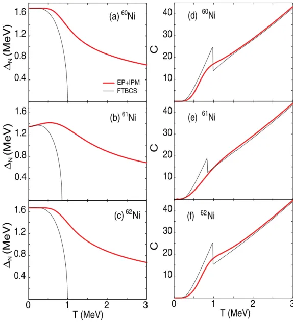
FIG. 1. Neutron pairing gaps[(a)–(c)] and total heat-capacitiesC[(d)–(f)] as functions ofT obtained within the EP+IPM (the thick solid line) and the FTBCS (the thin solid line) for60–62_{Ni isotopes.}

above-mentioned empirical formula in the region of excitation energyE∗<30 MeV. Including these effects of vibrational and rotational enhancements, the final total NLD is given as [25,29]

˜

ρ(E∗)=krotkvibω(E∗)/(σ

√

2π). (14)

By using the nuclear temperature ˜T(E)=[∂ ln ˜ρ(E)/∂E]−1_, which is defined from Eqs. (1) and (14), one finds from Eq. (2) the parameterB( ˜T) simply as

B( ˜T)=ρ˜(E∗)e−E∗/T˜. (15)

III. ANALYSIS OF THE NUMERICAL RESULTS The numerical calculations are carried out for60–62_{Ni and} 170–172_{Yb isotopes, whose single-particle spectra are taken} from the axially deformed Woods-Saxon potentials, following

the method described in Ref. [30]. By defining the nuclear shape in terms of a multipole expansion into spherical harmon-ics, this method diagonalizes a model Hamiltonian including the spin-orbit interaction and Coulomb potential for protons in the axially deformed harmonic-oscillator basis, which allows up to 19 harmonic-oscillator shells. The single-particle spectra used in the present calculations span a large space from the bottom of the potential up to the major shell with N =126 (five harmonic-oscillator shells). The neutron spectra are from around −39 and −40 MeV up to around 25 and 10 MeV, whereas the proton spectra are from around−34 and−33 MeV up to 30 and 19 MeV for Ni and Yb isotopes, respectively. The distances max

0.2

0.4

0.6

0.8

1.0

Δ

(MeV)

0.2

0.4

0.6

0.8

1.0

Δ

(MeV)

0.2

0.4

0.6

0.8

1.0

Δ

(MeV)

0

1

2

T (MeV)

3

(a) Yb

(b) Yb

(c) Yb

N Z

20

40

60

80

100

C

20

40

60

80

100

C

20

40

60

80

100

C

0

1

2

3

T (MeV)

(d) Yb

(e) Yb

(f) Yb

EP+IPM

FTBCS

FIG. 2. The same as in Fig.1but for Yb isotopes. The thick and thin lines stand for the EP+IPM and FTBCS results, respectively. from the mass calculations in Ref. [31] are employed. They

are estimated from the experimental values of the quadrupole transition probabilityB(E2; 2+₁ →0+₁) from the 2+₁ state to the 0+₁ one or the experimental binding energy. For 60–62Ni the values ofβ2 are determined asβ2=0,−0.13, and−0.2, respectively, whereas for 170,171_{Yb and} 172_{Yb these values} are determined as 0.295 and 0.296, respectively. The other parameters of the Woods-Saxon potential are the same as those reported in Ref. [30]. The values of the pairing interaction parameter G for neutrons and protons are chosen so that the exact neutron and proton pairing gaps obtained atT =0 reproduce the corresponding experimental values extracted from the odd-even mass differences [32]. For60–62_{Ni isotopes,} which are proton closed-shell nuclei (Z=28) (_Z=0), only neutron pairing is treated by using the values of GN chosen to be 0.475, 0.48, and 0.473 MeV, respectively. For170–172_Yb these values are G_N(G_Z)=0.25 (0.29), 0.284 (0.286), and 0.24 (0.29) MeV, respectively. The diagonalization of the pairing Hamiltonian is carried out for 12 doubly degenerate single-particle levels with six levels above and six levels below

the Fermi surface. A set of a total of 73 789 (69 576) eigenstates for the even (odd) particle number of each type of particles is obtained and employed to construct the exact CE partition function. The remaining portion of the single-particle spectrum outside this truncated space is treated within the IPM as has been discussed in the previous section.

10

10

10

10

10

ρ

(MeV )

-1

10

10

10

10

ρ

(MeV )

-1

0

5

10

15

20

E* (MeV)

10

10

10

10

ρ

(MeV )

-1

(a) Ni

(b) Ni

(c) Ni

HFBC positive parity HFBC negative parity HFBCS

Exp. data

~

~

~

FTBCS

SMMC

0

2

4

6

8

10

E* (MeV)

10

10

10

10

10

10

10

10

10

10

10

10

10

10

10

(d) Yb

(e) Yb

(f) Yb

EP+IPM

FIG. 3. Total level densitiesρas functions ofE∗obtained within the EP+IPM (the thick solid line) and the FTBCS (the thin solid line) in comparison with predictions of SMMC calculations (the triangles) [(a)–(c)], the HFBC calculations for the positive (the dashed lines) and negative parities (the dotted lines), and the HFBCS ones (the dashed-dotted lines). The experimental data for Ni and Yb isotopes are from Refs. [34,38,39], resepctively.

in the region aroundT_c, confirming that the phase transition is smoothed out [Figs. 1(d)–1(f)]. The increase in the heat capacities with T at high T also assures that the single-particle spectra employed in the calculations are sufficiently large.

Similar features are seen for Yb isotopes where the FTBCS heat capacities have two peaks located atT_c[Figs.2(d)–2(f)], which correspond to the collapse of the neutron and proton pairing gaps [Figs.2(a)–2(c)], whereas the exact results yield smooth curves, which monotonically decrease (the pairing gaps) or increase (the heat capacities) as increasingT.

The NLDs obtained within the EP+IPM (the solid lines) for Ni isotopes and shown in Figs. 3(a)–3(c) as functions of E∗ agree much better with the experimental data [34] than the predictions by the global microscopic calculations within the HFBC method for both negative (the dashed lines)

10-4

10-2

100

102

104

B(T)

(MeV )

-1

10-4

10-2

100

102

B(T)

(MeV )

-1

10-4

10-2

100

102

B(T)

(MeV )

-1

0 5 10 15

E* (MeV)

0 10 20 30 40 50

E* (MeV) (d1) Ni 60

(d2) Ni 60

(e1) Ni 61

(e2) Ni 61

(f1) Ni 62

(f2) Ni 62

-2 0 2 4

T (MeV)

~

-2 0 2 4

T (MeV)

~

-2 0 2 4

T (MeV)

~

0 5 10 15

E* (MeV)

0 10 20 30 40 50

E* (MeV) (a1) Ni 60

(b1) Ni 61

(c1) Ni 62

(a2) Ni 60

(b2) Ni 61

(c2) Ni 62

~

~

~

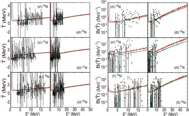
FIG. 4. Nuclear temperature ˜T, calculated from Eq. (1) by using the NLD ˜ρ(E∗) (14) and parameterB( ˜T) (15) as functions of excitation energyE∗for60–62_{Ni isotopes (the thick solid lines). The corresponding results obtained within the FTBCS are shown by the thin solid lines.} The data points are obtained by using the experimental NLDs from Ref. [34].

by the Hartree-Fock plus BCS (HFBCS) approach [36], the EP +IPM results in general have a steeper slope, which is lower at E∗7–7.7 MeV (10 MeV) for 60,61Ni (62Ni) and slightly higher at larger E∗ than that obtained within the

HFBCS. In the low-E∗ region the predictions by both the EP+IPM and the HFBCS agree well with the experimental data (within the experimental error bars). In the high-E∗_region

the EP+IPM results still are closer to the experimental data

0 1 2 3

T (MeV)

0 1 2

T (MeV)

0 1 2

T (MeV)

0 10 20 30 40 50

E* (MeV)

10-2

100

102

104

106

10-2

100

102

104

106

10-2

100

102

104

0 10 20 30 40 50

E* (MeV)

0 2 4 6 8

E* (MeV)

0 2 4 6 8

E* (MeV)

(d1) Yb

(d2) Yb

(e1) Yb

(e2) Yb

(f1) Yb

(f2) Yb

171 170

172

171 170

172

(a1) Yb

(a2) Yb

(b1) Yb

(b2) Yb

(c1) Yb

(c2) Yb

171 170

172

171 170

172

~

~

~

B(T)

(MeV )

-1

B(T)

(MeV )

-1

B(T)

(MeV )

-1

~

~

~

EP+IPM

IPM

₁₀

10

10

10

ρ

(MeV )

-1

0.2

0.4

0.6

0.8

1.0

1.2

1.4

10

10

10

B(T) (MeV )

-1

0

5

10

15

20

E* (MeV)

Ni

60

(a)

(b)

(c)

Yb

170

(d)

(e)

(f)

10

10

10

10

10

ρ

(MeV )

-1

0.5

1.0

1.5

2.0

2.5

T (MeV)

~

10

10

10

B(T) (MeV )

-1

10

0

5

10

15

20

E* (MeV)

T (MeV)

~

~

_~

~

~

FIG. 6. Comparison of NLD ˜ρ(14), temperature ˜T, which is calculated from Eq. (1) by using ˜ρ, and coefficientB( ˜T) (15) for60Ni and 170_{Yb (the solid lines) with their corresponding values obtained without pairing (the dashed lines).}

than the HFBCS ones especially for 60,61_{Ni. The prediction} by the shell-model Monte Carlo (SMMC) approach [37] is bracketed between the EP + IPM and the HFBCS results in the low-E∗ _{region but closer to the HFBCS one at}

highE∗.

For Yb isotopes, the total NLDs obtained within the EP+IPM and HFBC (after being renormalized) and shown in Figs.3(d)–3(f)agree quite well with the experimental data and generally better than the predictions by the HFBCS. The latter overestimates the experimental data for 170,172Yb at E∗ _{>2 MeV. For} 171_{Yb the HFBCS slightly overestimates} the experimental NLD at 0.5< E∗_{<2 MeV and}

underesti-mates it atE∗>5 MeV. Meanwhile, the FTBCS in general underestimates the experimental data, in particular, for the odd isotopes61Ni and171Yb.

The nuclear temperature ˜T, which was calculated by using the definition (1) and the total NLD ˜ρ(E∗) in Eq. (14) for 60–62_{Ni isotopes, is displayed in Figs. 4(a1)–4(c2) as a} function of E∗ from which panels (a1), (b1), and (c1) are the portions at low excitation energy (E∗ _{20 MeV) of the}

corresponding panels on their right, that is, (a2), (b2), and (c2).

The corresponding values of the parameterB( ˜T), which were calculated by using Eq. (15), are plotted in Figs.4(d1)–4(f2). The data points are obtained by using the same Eqs. (1) and (15) but with the experimental NLDs from Ref. [34] instead of ˜ρ(E∗) (14). The results in Figs. 4(a1)–4(c2) show that, except for the region of very low excitation energy below 1 MeV, the nuclear temperature ˜T increases almost linearly withE∗ but this increase is relatively slow so that ˜T can be approximated with a constant of around 1–1.5 MeV at E∗ within the energy interval where the data points are available. The values of ˜TFTBCSandB( ˜T)FTBCS, which are obtained by using ˜ρ(E∗)FTBCScalculated within the FTBCS, also are shown in Figs.4(a1)–4(f2)for comparison (the thin solid lines). At E∗_{5 MeV, the thin line, which describes the dependence}

A quite similar feature is also seen in 170–172_{Yb isotopes} as displayed in Fig.5where the data points were obtained by using the experimental NLDs from Refs. [38,39]. This figure also shows that the temperature ˜T remains nearly constant at around 0.5 MeV between E∗ 0.4 and 0.6 MeV up to E∗_{10 MeV, that is, within the original assumption on the}

validity of the CT model. TheE∗dependences of ˜TFTBCSand B( ˜T)FTBCSnow have two singular points, corresponding to the collapse of the FTBCS neutron and proton pairing gaps, below which B( ˜T)FTBCS is generally smaller than B( ˜T) obtained within the EP+IPM.

It can also be observed from these results that the values of the coefficient B( ˜T) obtained in odd-mass isotopes 61Ni and171Yb are about one order larger than the corresponding values in the neighboring even-even nuclei. The source of this difference is the pairing suppression at low excitation energy in odd-mass nuclei because of the blocking effect [33].

In Fig. 6 we compare the NLDs ˜ρ(E∗), temperature ˜T, and coefficientB( ˜T) obtained for60Ni and170Yb within the EP +IPM (the solid lines) with their corresponding values obtained within the IPM (the dashed lines), that is, without pairing. The figure shows that the slope of the NLDs obtained without pairing [the dashed lines in Figs. 6(a) and6(d)] is steeper than that of the results obtained with exact pairing. Consequently, the dependence of ˜T on the excitation energy E∗_{is depleted atE}∗_{<5 MeV [the dashed lines in Figs.6(b)}

and 6(e)], worsening the validity of the CT model in this region of low excitation energy. The corresponding values of the coefficient B( ˜T) become larger by around one and two orders atE∗>5 MeV for60Ni and170Yb, respectively. The slope of B( ˜T) obtained without pairing also gets steeper at E∗_{<5 MeV. AtE}∗ _{>5 MeV, pairing has almost no effect}

on ˜T because the lines describing theE∗dependences of the NLDs obtained by using exact pairing [the thick lines in Figs.3,

6(a), and6(d)], FTBCS pairing (the thin lines in Fig.3), and without pairing [the dashed lines in Figs. 6(a)and6(d)] are almost parallel to each other. This makes their derivatives over E∗_{almost identical, so are the values of ˜Tdefined from Eq. (1).}

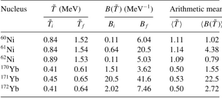
The arithmetic means T˜ of temperatures ˜T andB( ˜T) of the coefficients B( ˜T) within the intervals of excitation energyE_i∗E∗E_f∗ withE_i∗=1, E∗_f =20, and 10 MeV for nickel and ytterbium isotopes, respectively, are collected in TableI. For60Ni the arithmetic meanT˜ =1.11 MeV is slightly lower than the value found in Ref. [34] where it has been shown that the NLDs in 60Ni and 60Co can be quite well described by the CT model at a constant temperature of T =1.4 MeV up to E∗=20 MeV. Nonetheless, this value of temperature still is located well between T_i =0.84 andT_f =1.52 MeV obtained atE∗_i =1 andE_f∗ =20 MeV, respectively.

The choice of ˜T =1.4 MeV, proposed in Ref. [34], does not seem to be unique because any value of ˜T within the energy interval 1 MeV< E∗20 MeV, which is obtained from the same NLD ˜ρ(E∗) (14), whose corresponding to a coefficientB( ˜T) remains approximately constant within this energy interval, can serve as an alternative. To demonstrate this, in Fig.7(b), we show the coefficient B( ˜T) obtained at several temperatures [Fig.7(a)] to reproduce the NLD ˜ρ(E∗)

TABLE I. Arithmetic means_T˜of temperatures ˜T andB( ˜T) of the coefficientB( ˜T) in the energy intervalE_i∗E∗E_f∗ with E∗

i =1 MeV, whereas Ef∗=20 MeV for 60–62Ni and 10 MeV

170–172_{Yb isotopes. The values of ˜T}

iatEi∗and ˜Tf atEf∗ as well as

the corresponding valuesB_i≡B( ˜T_i) andB_f≡B( ˜T_f) of coefficient B( ˜T) (15) also are shown.

Nucleus T˜ (MeV) B( ˜T) (MeV−1) Arithmetic mean ˜

Ti T˜f Bi Bf T˜ B( ˜T)

60_{Ni 0.84 1.52 0.11 6.04 1.11 1.02}

61_{Ni 0.84 1.54 0.64 20.5 1.14 4.38}

62_{Ni 0.89 1.53 0.11 5.03 1.09 0.79}

170_{Yb 0.41 0.61 1.51 3.62 0.50 1.55}

171_{Yb 0.45 0.65 20.5 41.6 0.53 22.5}

172_{Yb 0.41 0.64 2.02 7.46 0.50 2.72}

in60Ni within the energy interval 0< E∗20 MeV. As seen in Fig.7(b), the lines showing the dependence ofB( ˜T) onE∗ obtained at ˜T =1.3, 1.4, and 1.52 MeV weakly change with E∗_{in the interval 5 MeVE}∗ _{20 MeV so that they can be}

approximated by corresponding constant values.

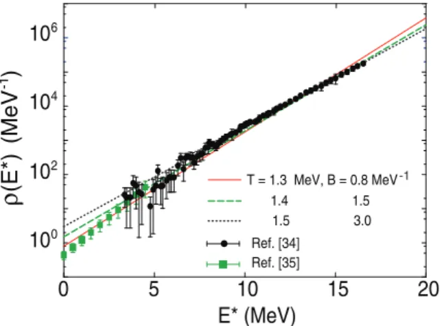
Shown in Fig.8are the predictions for the NLDρ(E∗) in 60_{Ni by the CT model (2) atT =1.3, 1.4, and 1.5 MeV for} which the corresponding constant (E∗-independent) values of the coefficient B are found so that the best fit to the experimental NLDs is achieved. As compared to the prediction

0

5

10

15 20

E* (MeV)

T (MeV)

~

0

1

2

10

10

10

B(T)

(MeV )

-1

(a)

(b)

Ti

Ti

<T>

<T>

Tf

Tf

1.4 1.3

1.3 1.4

~

0 5 10 15 20 E* (MeV)

10 0

10 2

10 4

10 6

ρ

(E*)

(MeV )

-1

T = 1.3 MeV, B = 0.8 MeV

1.4 1.5

1.5 3.0

Ref. [35] Ref. [34]

-1

FIG. 8. Comparison of NLDsρ(E∗) obtained from the CT model (2) atT =1.3 (the solid line), 1.4 (the dashed line), and 1.5 (the dotted line) MeV and experimental NLDs for60_Ni.

withT =1.4 MeV andB =1.5 MeV−1_{, the NLD obtained} with T =1.3 MeV and B=0.8 MeV−1 gives a better fit to the low-energy data [35]. The latter were extracted from the analysis of the experimental level scheme within the in-terval 0E∗ 4.613 MeV withT =0.9836±0.0952 and E0 =0.8242±0.2981 MeV, which corresponds to a value ofB=0.44₋+₀0._.18₁₁MeV−1in Eq. (2). The NLD obtained with T =1.5 MeV andB =3.0 MeV−1agrees slightly better with the data in the region 10 MeVE∗20 MeV. However, all three predictions overall agree with the experimental data within the whole interval 0< E∗ 20 MeV. In other words, one may say that, for60Ni, the CT model of the NLD is valid up toE∗=20 MeV with any constant value of temperature within the interval 1.3T 1.5 MeV.

IV. CONCLUSIONS

In the present paper, by using the NLD predicted within the EP+IPM method, which agrees well with the experimental

data, the nuclear temperature ˜T is calculated from the deriva-tive of the logarithm of NLD (1). This temperature ˜T increases almost linearly with the excitation energy E∗. However this increase is relatively slow so that ˜T can be considered as a constant of around 0.5 MeV at 0< E∗10 MeV for ytterbium isotopes. Meanwhile, in 60Ni, the CT model can describe rather well the experimentally extracted NLD with a constant temperature between 1.3_T˜ _{1.5 MeV up} to E∗=20 MeV, which is much higher than the particle separation threshold. This feature is in excellent agreement with the experimental finding of Ref. [34]. It is also shown that pairing plays an important role in maintaining this nearly constant value of temperature at low excitation energy. In this way, the EP + IPM offers a consistent description of the NLD, which goes smoothly from the low-energy region E∗_{5 MeV to the higher one (up to 20 MeV for Ni isotopes}

and 10 MeV for Yb isotopes) without the need for matching the CT model at low energy and the Fermi-gas one at high energy as often performed by using the composite level-density formula [5]. As a matter of fact, the values of the matching energyE_xdefined from the composite level-density formula by using Eq. (26) and Table III in Ref. [5] are 7.49, 6.16, and 7.53 MeV for Ni isotopes withA=60, 61, and 62, respectively. For 170–172_{Yb they are 4.67, 4.06, and 4.74 MeV, respectively. Last} but not least, the fact that the NLD at low excitation energy, even atE∗ =0, can be described well by the CT model at a constant nonzero temperature also supports the suggestion of introducing a ground-state’s effective temperature [40].

ACKNOWLEDGMENTS

N.D.D. is grateful to L. G. Moretto (LBL), K. Yazaki (RIKEN), and V. Zelevinsky (MSU) for valuable discussions and suggestions. The numerical calculations were carried out using theFORTRAN IMSLLibrary by Visual Numerics on the RIKEN supercomputer HOKUSAI-GreatWave System. This work was funded by the National Foundation for Science and Technology Development (NAFOSTED) of Vietnam through Grant No. 103.04-2017.69.

[1] T. Ericson,Adv. Phys.9,425(1961).

[2] T. Rauscher and F. K. Thielemann,At. Data Nucl. Data Tables

75,1(2000).

[3] T. Rauscher, F. K. Thielemann, and K. L. Kratz,Phys. Rev. C

56,1613(1997).

[4] H. A. Bethe,Phys. Rev.50,332(1963);Rev. Mod. Phys.9,69

(1937).

[5] A. Gilbert and A. G. W. Cameron,Can. J. Phys.43,1446(1965). [6] A. V. Voinov, B. M. Oginni, S. M. Grimes, C. R. Brune, M. Guttormsen, A. C. Larsen, T. N. Massey, A. Schiller, and S. Siem,Phys. Rev. C79,031301(R)(2009).

[7] M. Guttormsen, B. Jurado, J. N. Wilson, M. Aiche, L. A. Bernstein, Q. Ducasse, F. Giacoppo, A. Görgen, F. Gunsing, T. W. Hagen, A. C. Larsen, M. Lebois, B. Leniau, T. Renstrøm, S. J. Rose, S. Siem, T. Tornyi, G. M. Tveten, and M. Wiedeking,

Phys. Rev. C88,024307(2013).

[8] M. Guttormsen, L. A. Bernstein, A. Görgen, B. Jurado, S. Siem, M. Aiche, Q. Ducasse, F. Giacoppo, F. Gunsing, T. W. Hagen,

A. C. Larsen, M. Lebois, B. Leniau, T. Renstrøm, S. J. Rose, T. G. Tornyi, G. M. Tveten, M. Wiedeking, and J. N. Wilson,Phys. Rev. C89,014302(2014).

[9] L. G. Moretto et al., J. Phys.: Conf. Ser. 580, 012048

(2015).

[10] L. G. Moretto,Phys. Lett.40B,1(1972).

[11] R. Rossignoli, P. Ring, and N. Dinh Dang,Phys. Lett. B297,9

(1992); N. Dinh Dang, P. Ring, and R. Rossignoli,Phys. Rev. C

47,606(1993).

[12] V. Zelevinsky, B. A. Brown, N. Frazier, and M. Horoi,Phys. Rep.276,85(1996).

[13] D. J. Dean, S. E. Koonin, K. Langanke, P. B. Radha, and Y. Alhassid,Phys. Rev. Lett.74,2909(1995).

[14] N. Dinh Dang and A. Arima,Phys. Rev. C68,014318(2003); N. Dinh Dang and V. Zelevinsky,ibid.64,064319(2001); N. Dinh Dang,Nucl. Phys.A784,147(2007).

[15] N. Dinh Dang and N. Quang Hung,Phys. Rev. C77,064315

[16] N. Quang Hung and N. Dinh Dang,Phys. Rev. C79,054328

(2009).

[17] R. Sen’kov and V. Zelevinsky,Phys. Rev. C93,064304(2016). [18] N. Quang Hung, N. Dinh Dang, and L. T. Quynh Huong,Phys.

Rev. Lett.118,022502(2017).

[19] A. Volya, B. A. Brown, and V. Zelevinsky,Phys. Lett. B509,

37(2001).

[20] N. Quang Hung and N. Dinh Dang,Phys. Rev. C81,057302

(2010).

[21] N. Quang Hung and N. Dinh Dang,Phys. Rev. C82,044316

(2010).

[22] Y. Alhassid, G. F. Bertsch, and L. Fang,Phys. Rev. C68,044322

(2003).

[23] H. Nakada and Y. Alhassid,Phys. Rev. Lett.79,2939(1997). [24] W. Dilg, W. Schantl, H. Vonach, and M. Uhl,Nucl. Phys.A217,

269(1973).

[25] A. R. Junghanset al.,Nucl. Phys. A629,635 (1998); M. N. Nasrabadi and M. Sepiani,Acta Phys. Pol., B45,1865(2014). [26] A. V. Ignatyuk,The Statistical Properties of the Excited Atomic Nuclei (Energoatomizdat, Moscow, 1983); S. Bjørnholm, A. Bohr, and B. Mottelson, Proceedings of the Symposium on Physics and Chemistry of Fission(IAEA, Vienna, 1974), Vol. I, p. 367.

[27] A. S. Iljinov,Nucl. Phys.A543,517(1992).

[28] S. Goriely, S. Hilaire, and A. J. Koning,Phys. Rev. C78,064307

(2008).

[29] R. Capoteet al.,Nucl. Data Sheets110,3107(2009).

[30] S. Cwiok, J. Dudek, W. Nazarewicz, J. Skalski, and T. Werner,

Comput. Phys. Commun.46,379(1987).

[31] P. Möller, J. R. Nix, W. D. Myers, and W. J. Swiatecki,Atomic Data Nucl. Data Tables59,185(1995).

[32] N. Zeldes, A. Grill, and A. Siemievic, Mat. Fys. Skr. Dan. Vid. Selsk.3, 5 (1967); A. Bohr and B. Mottelson,Nuclear Structure (Benjamin, NY, 1969), Vol. 1, p. 170.

[33] N. Quang Hung, N. Dinh Dang, and L. T. Quynh Huong,Phys. Rev. C94,024341(2016).

[34] A. V. Voinov, S. M. Grimes, C. R. Brunes, T. Massey, and A. Schiller,EPJ Web Conf.21,05001(2102).

[35] https://www-nds.iaea.org/RIPL-3/

[36] P. Demetriou and S. Goriely,Nucl. Phys.A695,95(2001). [37] M. Bonett-Matiz, A. Mukherjee, and Y. Alhassid,Phys. Rev. C

88,011302(R)(2013).

[38] A. Schiller, A. Bjerve, M. Guttormsen, M. Hjorth-Jensen, F. Ingebretsen, E. Melby, S. Messelt, J. Rekstad, S. Siem, and S. W. Ødegård,Phys. Rev. C63,021306(R)(2001).

[39] U. Agvaanluvsan, A. Schiller, J. A. Becker, L. A. Bernstein, P. E. Garrett, M. Guttormsen, G. E. Mitchell, J. Rekstad, S. Siem, A. Voinov, and W. Younes,Phys. Rev. C 70, 054611

(2004).