National Income Accounting When Firms Insure Workers
Barney Hartman-Glaser∗, Hanno Lustig†, and Mindy X. Zhang‡
March 4, 2016
Preliminary and Incomplete
Abstract
We analyze national income accounting in an equilibrium model of industry dynamics with long-term contracts between risk-averse workers and heterogeneous firms. In our model, firms insure workers against firm-specific productivity shocks. We use this model as a laboratory for analyzing the impact of firm-level risk on the stationary distribution of rents. An increase in firm-level risk always increases the aggregate capital share in the economy, but may lower the average firm’s capital share. Because of selection, the aggregate capital share reported in national income accounts produces a biased estimate of ex ante profitability of firms which determines compensation. Workers effectively pay a larger insurance premium to the owners of capital.
Keywords: Selection, Capital Share, Labor Share, National Income Accounting.
∗
UCLA Anderson School, [email protected]
†
Stanford GSB and NBER, [email protected]
‡
1
Introduction
Over the last decades, publicly traded U.S. firms have experienced a large increase in
firm-specific volatility (see, e.g., Campbell, Lettau, Malkiel, and Xu, 2001; Comin and Philippon, 2005;
Zhang, 2014; Herskovic, Kelly, Lustig, and Van Nieuwerburgh, 2015) that is apparent in firm-level
cash flows and returns. We explore the impact of changes in firm-level risk on the distribution
of rents between workers and shareholders in an equilibrium model of industry dynamics with
heterogeneous firms and workers.
Since shareholders of publicly traded firms can diversify idiosyncratic firm-specific risk away,
while risk-averse workers cannot, it is efficient for firms to provide workers with insurance against
firm-specific risk. We analyze the simplest insurance contract in an equilibrium model of industry
dynamics (see, e.g., Hopenhayn, 1992). Ex ante identical firms that are subject to idiosyncratic
risk insure the workers. We use this model as a laboratory to analyze the impact of changes in
firm-level risk on the distribution of rents.
Standard national income accounting applied inside this model yields a novel perspective on
capital share dynamics. Workers can only contract with a single new firm. The worker’s
compen-sation is set such that the net present value of starting a new firm is zero. This present value is
obtained by discounting all future productivity paths for the new firm, but the national income
accounts only integrate over all firms that are currently alive. As a result, the aggregate capital
share calculation puts more probability mass on the right tail than the NPV calculation. This puts
the average worker at a disadvantage as firm-level risk increases and the right tail of the firm size
distribution grows. She captures a smaller fraction of aggregate rents as a result. In our model, an
increase in risk invariably increases the capital share.
Selection is at the heart of this mechanism.1 Our main result is closely related to Hopenhayn
(2002)’s observation that selection biases average Tobin’s Q estimates for industries above one.
Because of selection, the capital share computed in national income accounts also produces a
biased estimate of the ex ante profitability of new firms. An increase in selection increases the size
of the bias. That explains the measured divergence between aggregate compensation and profits:
Compensation is tied to ex ante profitability, not the ex post realized one.
1
This result has a natural insurance interpretation. When idiosyncratic risk increases, workers
effectively pay a larger idiosyncratic insurance premium to shareholders, leading to an increase in
the aggregate capital share, even though the shareholders are risk-neutral. Our selection mechanism
has interesting cross-sectional implications. Only the capital share of the largest firms in the right
tail increases as risk increases. The capital share of the smallest firms will actually decrease. As a
result, the average capital share across all firms will tend to decrease.
Between 1960 and 2010, the U.S. labor share of total output in the non-farm business sector
of the U.S. economy has shrunk by 15 percent. We find that the shrinkage in the labor share
is concentrated among the largest firms in the U.S. The average labor share of publicly traded
companies has not declined. This new cross-sectional evidence is consistent with the selection
mechanism: The divergence between the average and the aggregate labor share is a key prediction
of selection. The main competing hypothesis is that firms are increasingly substituting capital for
labor (see, e.g., Karabarbounis and Neiman, 2013) in response to declines. As far as we know, this
mechanism does not predict a divergence between the average and aggregate labor share.
There is a large literature on optimal risk sharing contracts between workers and firms (see
Thomas and Worall, 1988; Holmstrom and Milgrom, 1991; Kocherlakota, 1996). This literature
has analyzed the trade-off between insurance and incentives. We analyze the case of complete
insurance as our benchmark. When we introduce moral hazard, limited commitment and related
frictions, our mechanism will be mitigated.
2
Model
In this section we present a model in which firms produce cash flows according to a simple
production function. To keep the analysis simple, we abstract from physical capital and unskilled
labor. Adding these factors would not change any of the main results, but it would complicate the
analysis.
Importantly, the owners of the firm hold an option to cease operations when productivity falls.
This is the classic abandonment option that has been well studied in the real options literature.
As is standard in that literature, increasing the volatility of the firms cash flows increases the value
firm ceases operations. We then characterize the stationary distribution of firms implied by the
optimal abandonment policy. Increasing (idiosyncratic) cash flow volatility leads more firms to
delay abandonment and survive long enough to become very productive. As such, the average
across firms of the capital share of profits can be increasing in volatility.
2.1 Environment
The economy is populated by a measure of ex ante identical firms each producing cash flow
Xidt given by
dXi =µXidt+σXidZi−XidNti
whereZi is a standard Brownian motion independent across firms andNiis a Poisson process with
intensity λ. When a jump is realized, Xi jumps to zero, and the firm exits.
Each firm is owned by a investor and requires a manager to operate. We assume investors
are risk-neutral and discount cash flows at the risk free rate r while managers value a stream of
payment {ct}t≥0 according to the following utility function
U({ct}t≥0) =E
Z ∞
0
e−rtu(ct)dt
,
whereu0(c)≥0 andu00(c)>0.
Firms can exit at the discretion of the investor. When a firm exit, its investor receives liquidation
value normalized to zero. New firms are created at each date twith Pareto density
f(X) = ρ
X1+ρ; X∈[Xmin,∞)
over initial productivity where Xmin > 0. This distribution implies that the log-productivity of
entering firms is exponentially distributed with parameterρ >1.
The owner of the firm enters into a long-term contract with the manager at the inception of
the firm. Formally, this contract can be denoted by a process {ct}t≥0 determining payment to
the manager of ct at time t. We assume that the investor cannot commit to continue to pay the
manager once the firm has ceased operations. We also assume that the manager does not have
entering firm and signs a new contract.
We denote the utility the manager receives upon entering this market by U0, which is also the
manager’s reservation utility. The investor takes U0 as exogenously given. We denote by τ the
stopping time at which the investor chooses to cease operation. The investor’s problem is thus
max
τ,c E
Z τ
0
e−rt(Xt−ct)dt
such that
U0≤E
Z τ
0
e−rtu(ct)dt+e−rτU0
.
Intuitively, since the manager is risk-averse, the investor is risk-neutral, and there is no need of any
incentives, the optimal contract will call for full insurance. As such, it is without loss of generality
to restrict attention to contracts that offer the manager a fixed wagecuntil the firm exits, at which
point the manager reenters the market and receives her outside option. Thus, we can simplify the
investors problem to
V(X;c) = max
τ E
Z τ
0
e−rt(Xt−c)dt
, (1)
whereV(X;c) is the value of operating a firm with current productivityXgiven a manager contract
c. The paymentcto the manager then acts as a fixed cost. As such, the investor in a given firm will
choose to exit if productivity X is low enough as in the classic problems of optimal abandonment
considered in the real options literature. It is without loss of generality to restrict attention to firm
exit times that are given by threshold rules of the form
τ = inf{t|Xt≤X¯ ordNt= 1} (2)
for some ¯X≥0.
To pin down the level of compensation to manager, we assume that there is free entry into
the market to create new firms. Moreover, we assume that when an investor creates a new firm,
she is matched with a manager and must sign a long term contract prior to learning the initial
the firm in expectation as follows. That is c∗solves
E[V(X, c∗)] =
Z ∞
¯ X(c∗)
V(X;c∗)f(X)dx=P, (3)
whereP is the cost of starting a new firm andV(X;c) is the value of operating a firm with current
productivity X given a manager contractc. Hence, the manager’s compensation is tied to the ex
ante profitability of new firm. Atkeson and Kehoe (2005) use a similar approach to determine the
manager’s compensation in their study of organizational capital. Since we have abstracted from ex
ante heterogeneity, the perfect insurance contract produces no dispersion in compensation across
managers. We will return to the question of dispersion in managerial compensation in Section ??. Note that the investor can choose not to start the firm if the wage is too high given the outcome
of X. Thus the lower bound on the support of the integral in equation (3) is the threshold ¯X(c)
below which the investor chooses to exit. Anequilibrium is then a value functionV(X), a manager
wagec∗, and a firm exit threshold ¯X that satisfy equations (1)-(3).
2.2 Optimal Abandonment and the Equilibrium Wage
To solve for the firm value function and exit policy of the investor, we use standard techniques
from the real options literature. An application of Ito’s formula and the dynamic programing
principal imply that V(X;c) must satisfy the following ordinary differential equation
(r+λ)V(X;c) =X−c+µX ∂
∂XV(X;c) + 1 2σ
2X2 ∂2
∂X2V(X;c), (4)
with the boundary conditions
V( ¯X(c);c) = 0, (5)
∂
∂XV( ¯X(c);c) = 0, (6)
lim X→∞
V(X;c)−
X r+λ−µ −
c r+λ
= 0. (7)
Conditions (5) and (6) are the standard value matching and smooth pasting conditions pinning
Xttends to infinity, abandonment occurs with zero probability and the value of the firm must tend
to the present value of a growing cash flow less a fixed cost.
The solution to equations (4)-(7) is given by
¯
X(c) = η η+ 1
c(r+λ−µ)
r+λ (8)
V(X;c) = X r+λ−µ−
c r+λ−
¯
X(c) r+λ−µ −
c r+λ
X ¯ X(c) −η (9) where η= µ−1
2σ
2+q(µ− 1
2σ2)2+ 2(r+λ)σ2
σ2 .
Note that an increase in firm-level volatilityσ invariably lowers the abandonment threshold, simply
because an increase in volatility raises the option value of keeping the firm alive. This feature of
the abandonment option will play key role in our analysis as will become apparent when we discuss
the stationary distribution of firm size. Specifically, an increase in firm-level volatility will lead to
a increase mass of firm’s that delay exit, increasing the mass of firms that have low productivity as
well the mass of firms that survive long enough to achieve high productivity.
Given the solution for firm value conditional on a manager wage c as well as our assumption
on the entry distribution of new firms, we can solve equation (3) for the equilibrium manager
compensation. We have
c∗=
P(r+λ)(ρ−1)(ρ−η) η
η(r+λ−µ) (η+ 1)(r+λ)
ρ−ρ−11
. (10)
Equations (8)-(10) characterize the equilibrium of the model and set the stage for our analysis of
national income accounting.
3
The Firm Size Distribution
In this section we characterize the stationary distribution of firm size and use it to compute
various moments of interest. In particular, we study how the total and average capital share relate
3.1 The Kolmogorov Forward Equation
We useφto denote the stationary distribution ofx= logX. To remain stationary, the expected
change via inflow and outflow in the measure of firms at a given level of x must be equal to the
measure of firms that exogenously die at the rateλless the measure of firms that exogenously enter
at the rate g(x) (see p. 273 in Dixit and Pindyck, 1994). This leads to the following Kolmogorov
forward equation forφ(x)
1 2σ
2φ00 (x)−
µ−1
2σ
2
φ0(x)−λφ(x) +g(x) = 0. (11)
where
g(x) =ρe−ρx.
is the entry density of x. A similarly argument gives a boundary condition for φ(x) at the exit
barrier ¯x
φ(¯x) = 0. (12)
The solution to equations (11) and (12) is given by
φ(x) = 1 ρ
2ρ2σ2+ρ(µ− 1
2σ2)−λ
e−γ(x−x¯)−ρ¯x−e−ρx (13)
forx∈[log[x],∞), where
γ =
−(µ−1 2σ2) +
q
(µ−1
2σ2)2+ 2σ2λ
σ2 . (14)
Figure 2 plots the stationary distribution of firm productivity for different levels of σ. The other
parameters are calibrated atr = 5%, µ= 2%, λ=.05, ρ= 3, p= 1. Asσ increases, the stationary
distribution shifts to the left and becomes more diffuse, with a fatter right tail. The shift to the
left is due to the fact that as firm-level volatility increase, the value of the option to wait to exit
increases, and the optimal point at which the investor chooses to exit necessary decreases. The
effect of firm-level volatility on the shape of φ(x) visible in figure 2 is born out by examining the
kurtosis of the log size distribution as we increase σ. Asσ increases, the right skewness increases
from 0.12 to 2.74 and the excess kurtosis of the log size distribution increases from 0.15 to 7.31.
This overall widening of the distribution with a fattening of the left tail comes from two effects.
First there is a direct effect of σ on the dispersion of the distribution of firm size. When
firm-level productitivity is more volatile, the stationary distribution of firms must be more dispersed.
This is evident by examining the dependence of γ on σ. The second effect operates through the
abandonment option. When the option to wait to exit becomes more valuable, more firms delay
exit, and as a result more firms survive long enough to become very productive. As a result the
right tail of the distribution becomes fatter. In the next section, we show that this effect has
important implications for national income accounting.
3.2 Capital Share and Ex Post Profitability
Armed with this stationary distribution, we can do national income accounting inside our model.
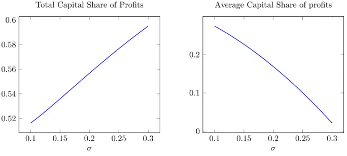
We use this stationary distribution to calculate the total and average profit share for a range of σ.
Specifically, we use the stationary distribution to calculate the aggregate capital share:
Total Capital Share of Profits = Π = E[X−c] E[X]
=
R∞
¯ x (e
x−c)φ(x)dx
R∞
¯
x exφ(x)dx
,
and the average capital share:
Average Capital Share of Profits =E
X−c X = Z ∞ ¯ x
ex−c ex
φ(x)dx.
Given the exponential entry distribution given above, the aggregate capital share is independent
of cand available in closed form:
Π = 1−
r+λ r+λ−µ
ρ−1 ρ
γ2−1
γ2
η+ 1 η
(15)
∂Π ∂σ =−
r+λ r+λ−µ
ρ−1 ρ
η+ 1 η
1 γ22
∂γ2
∂σ −
γ2−1
γ2 1 η2 ∂η ∂σ (16)
So ∂Π/∂σ is positive if and only if
η(η+ 1)∂γ2
∂σ ≤γ2(γ2−1) ∂η
∂σ. (17)
It is straightforward to show that η(η+ 1)∂η∂σ ≤0 and γ2(γ2−1)∂γ∂σ2 ≤0, , so to verify (17), it is
equivalent to verify
η(η+ 1)∂γ2
∂σ
γ2(γ2−1)∂σ∂η
≥1. (18)
After considerable algebra, one can show that
η(η+ 1)∂γ2
∂σ
γ2(γ2−1)∂η∂σ
=
q
(µ−12σ2)2+ 2(r+λ)σ2
q
(µ− 1
2σ2)2+ 2λσ2
>1 (19)
which verifies that ∂Π/∂σ >0. Hence, in our model, the aggregate capital share always increases
as volatility increases.
Figure 3 plots a calibrated example. The figure plots the total and average capital share of profit
as a functions ofσ. We use the following parameter values: r = 5%, µ= 2%, λ=.05, ρ= 3, p= 1.
We can see that the total capital share of profits is increasing in σ while the average capital share
of profits is decreasing. The intuition is as follows. Asσ increases, the value of the option to delay
abandonment increases, and hence the optimal threshold at which firms exit decreases. Holding
the total measure of firms fixed, this means that the distribution of profits becomes more dispersed.
The increase in mass of firms in the right tail of the firm size distribution increases the total profit
share, because the profit share measures the ex post profitability of existing firms. This is effectively
a selection bias. The profit share of entering firms is set by setting the NPV of the investor’s stake
in the firm to zero. This NPV calculation integrates over all possible future paths for firm-level
productivity, including those that lead the investor to choose to exit. In contrast, the stationary
distribution of existing firms only consider firms that have survived. Surviving firms necessarily
have a higher capital share of profits, otherwise the investor would have chosen to exit.
increase in mass of firms that delay exist means that there will be more firms with a low capital
share. Thus and increase in firm-level volatility can decrease the average profit share. This is in
contrast to the effect one would expect to see if the increase in total capital share of profits is due
to a greater growth rate in the value of capital relative to wages that may follow the substitution
of capital for labor. In that case, one would expect both the total and average capital share to
increase.
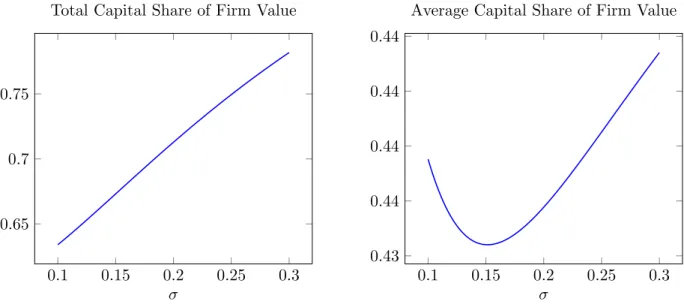
We can also examine the capital share of firm value, with similar results as for profits. Figure
4 plots the total and average capital share of firm value derived from the model.
4
Firm Performance and Managerial Compensation
In this section we allow the manager some exposure firm performance. Specifically we assume
that the managers contract takes the following simple affine form
ct=βXt+w (20)
whereβ is some exogenously given constant andwis set in equilibrium in the same manner as total
wages are set above. We can think of this contract as consisting of some profit sharing component
given by β and some fixed wage given by w. Under this contract, for a given fixed wage w, the
investors problem is
max
τ
Z τ
0
e−rt((1−β)Xt−w)dt
. (21)
Again, standard arguments imply that the investor’s value functionV(X) must statisfy the following
ODE
(r+λ)V = (1−β)X−w+µXV0+1 2σ
with the boundary conditions
V( ¯X) = 0, (23)
V0( ¯X) = 0, (24)
lim X→∞
V(X)−
(1−β)X r+λ−µ−
w r+λ
= 0. (25)
This problem is essentially the same as one given in equations (??)-(??), up to a scaling of the
leading term by a factor of (1−β). Thus, the solution to equation (22)-(25) is
¯ X =
1 1−β
η η+ 1
w(r+λ−µ) r+λ
V(X) = (1−β)X r+λ−µ −
c r+λ−
(1−β) ¯X r+λ−µ−
c r+λ
X ¯ X
−η
whereη is defined as above.
5
Empirical Evidence
In this section, we present empirical evidence on the joint dynamics of risk sharing and capital
share dynamics. We show the findings are consistent with the selection mechanism.
5.1 Data
Our baseline results are from analyzing two sources of data. To obtain cross-sectional evidence,
we use widely available accounting data from Compustat Fundamentals Annual, which includes all
publicly-traded firms. The sample is from 1960 to 2014. We exclude financial firms with SIC codes
in the interval 6000-6799, and also exclude firms whose sales, employee numbers and total asset
values are negative. We examine the distribution of factor share of output in the publicly traded
firm sample.
The capital income of the firm is measured by operating income before depreciation (OIBDP).
OIBDP represents sales/turnover (SALE) minus operating expenses including the cost of goods
to sales2. We use the ratio of the cost of labor to sales as the measure of labor share of output. The
cost of labor is the staff expenses – total (XLR) in Compustat. However, the limitation of XLR
is that XLR in Compustat is sparse with roughly 13% firm-year observations in the sample. We
then follow Donangelo, Gourio, and Palacios (2015) to construct the extended labor cost. We first
estimate the average labor cost per employee (XLR/EMP) within industry for each year using the
available XLR observations, and then labor cost of a firm with missing XLR equals the number of
employees times the average labor cost per employee of the same industry3 during that year.
We also obtain measures of labor share from U.S. Bureau of Labor Statistics. See Data Appendix
for detailed description. Labor’s share in current dollar output is the ratio of labor compensation
paid in that sector to current dollar output. Labor compensation is measured as all direct payments
to labor: wage and salary accruals (including executive compensation), commissions, tips, bonuses,
and payments in kind representing income to the recipients, and supplements to these direct
pay-ments. Supplements consist of employer contributions to funds for social insurance, private pension
and health and welfare plans, compensation for injuries, etc.
5.2 Time Series Evidence
In this section, we examine the capital share dynamics over time. Firm level volatility has
increased over the past five decades (Comin and Philippon (2005), Zhang (2014), Herskovic et al.
(2015)). Figure 5 confirms the time series results of firm-level volatility. The measure of cash flow
volatility and stock return volatility has almost doubled over the period 1960-2010. The rising
firm-level volatility is a very robust fact using other firm-level variables (Comin and Philippon
(2005)).
Let us first look at the firm size distribution in our sample. We estimate the power law exponent
of the size distribution over time. Following the literature, the power law exponent is the slope of
the right tail using the top n4 firms in a given year, plotted in Figure 6. The higher the coefficient
2Ideally, capital share should be computed using value added as denominator. However, the cost of material and
the cost of labor are not reported separately in the sample. Instead of using different ways to estimate the cost of labor or the cost of material which leads to many negative value added at the tail, we will stick to sales as the measure of output.
3We follow Donangelo et al. (2015) and use Fama-French 17 industry classifications. The result is robust using
2-digit SIC code.
4We usen = 100 given that out sample starts in 1960 with less than 600 firms. We applyn= 200,300 to the
ξ, the lower the probability of finding a firm with size larger than the cutoff X, i.e. the fatter the
right tail of the size distribution. The total size distribution of the publicly traded firms is relatively
stable, but becomes more dispersed over time.
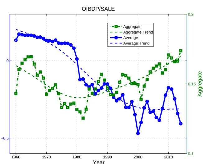
For most of our analysis, we focus on the capital share of output. Figure 7 plots the average and
aggregate capital share in the publicly traded firm sample. The average capital share is the sample
mean of capital share for a given year. As the firm-level volatility increases, the aggregate capital
share and the average capital share diverge. The aggregate capital share equals the sum of capital
income (OIBDP) across all the firms divided by aggregate sales. The average capital share drops
from 0.13 in 1960 to -0.40 in 2014, while the aggregate capital share increases with a less dramatic
scale, from 0.14 in 1960 to 0.17 in 2014. The presence of the contrasting trends in capital share
is consistent with the mechanism we highlight in our model. Specifically, the trends we observe in
the data a consistent with changes in firm-level volatility causing a shift in the distribution of firm
size that favors the owners of capital
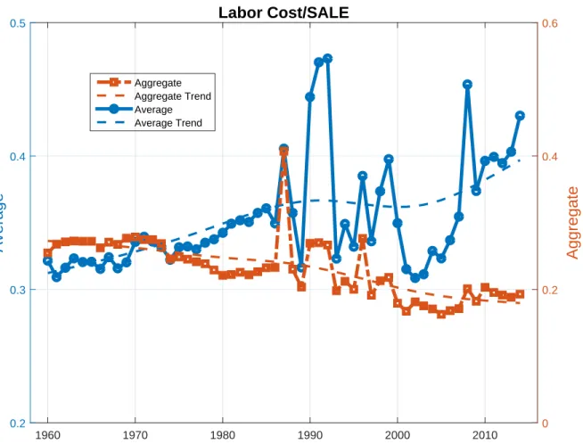
We find similar patterns in the labor share dynamics. The aggregate labor share of output in
the non-farm business sector has declined by 15%. However, the the trend of the average labor
share of output in the publicly traded firm sample did not decline. Figure 8 shows the time series of
both the average and the aggregate labor share in our sample using the estimated labor cost. The
average labor share rises from 0.32 in 1960 to 0.4 in 2014, while the aggregate labor share drops
from 0.25 to 0.19 during the same period of time.
5.3 Cross Sectional Evidence
We present more cross sectional evidence to support the selection mechanism. As volatility
increases over time, the value of option to abandon increases. Firms delay to exit and the right tail
of the size distribution also becomes heavier, so the simple average capital share declines over time.
We find a strong selection effect in the data. Figure 9 presents the cross-sectional evidence. All
firms are sorted into five groups based on their total assets. Within each group, we compute the
average capital share. The average capital share tends to decline more in the smaller size quintiles.
Aggregate capital share increases in total, but the increase in profitability mainly happens in the
larger firms. Over the period from 1960 to 2014, firm-level volatility has gone up, and hence small
During the same period, we find that the capital share of the large firms (group 5) remains stable.
The dispersion of capital share across size groups increases as the selection effect is stronger when
volatility increases, implying that the selection comes from the abandon decisions of firms on the
right tail of size distribution.
To address the concern of changing composition of public firm sample, we examine the
distribu-tion of capital share controlling for industries and cohort effects. We examine four main industries
in this paper: consumer goods, manufacturing, health products and information, computer and
technology (high tech) industry. The definition of consumer goods, manufacturing and health
products are taken from Fama-French 5 industry classification. The high tech industry definition
is from BEA Industry Economic Accounts5. We fix the definitions of industries over time, and sort
firms into five different size groups within each industry. We find similar cross-sectional patterns
within each industry: the dispersion of capital share across size groups increases over the last five
decades, while the more significant decline in capital share happens in the smaller size quintiles.
We also see stronger selection effect in the high tech industry and in the health products industry
which have relatively high firm-level volatility. Table A3 summarizes capital share distributions
for the four main industries. When comparing the capital share distributions across indsutries, the
changing firm-level volatility does not only shift the distribution of profitability, but also has impact
on the dispersion of the profitability with most of it from the right tail of the size distribution.
Very similar to what we find in the full sample analysis, the profitability of the largest size group
exhibits small variations across industries.
6
Conclusion
We propose a mechanism whereby an increase in firm-level volatility can have important effects
on national income accounting. A firm’s owner insurance it’s manager against firm-level
productiv-ity shocks. As a result, that owner may choose to exit if productivproductiv-ity becomes too low. The level
of the manager’s compensation is set based on expected firm value–which necessarily integrates
over paths that end in exit. In contrast, when accounting for income, one typically integrates over
surviving firms which necessarily feature lower capital shares of profit. This leads to an difference
5The high tech industry is classified using NAICS, consisting of computer and eletronic products, publishing and
between the aggregate capital share of income, which is calculated ex post, and the capital share of
value at the origination of firm, which is calculated ex ante. When firm-level volatility increases, the
difference can increase, increasing the aggregate capital share and decreasing the average capital
share. We also present time series and cross sectional evidence for Compustat firms consistent with
References
Atkeson, A., Kehoe, P., 2005. Modeling and measuring organizational capital. Journal of Political Economy 113, 1026–1053.
Campbell, J. Y., Lettau, M., Malkiel, B. G., Xu, Y., 2001. Have individual stocks become more volatile? an empirical exploration of idiosyncratic risk. The Journal of Finance 56 (1), 1–43. URLhttp://dx.doi.org/10.1111/0022-1082.00318
Comin, D., Philippon, T., 2005. The rise in firm-level volatility: Causes and consequences. NBER Macroeconomics Annual.
Dixit, A. K., Pindyck, R. S., 1994. Investment under uncertainty. Princeton university press.
Donangelo, A., Gourio, F., Palacios, M., 2015. Labor share and the value premium. Tech. rep.
Herskovic, B., Kelly, B. T., Lustig, H. N., Van Nieuwerburgh, S., 2015. The common factor in idiosyncratic volatility: Quantitative asset pricing implications. Journal of Financial Economics.
Holmstrom, B., Milgrom, P., 1991. Multitask principal-agent analyses: Incentive contracts, asset ownership, and job design. Journal of Law, Economics, & Organization 7, 24–52.
URLhttp://www.jstor.org/stable/764957
Hopenhayn, H., 2002. Exit, selection, and the value of firms. Journal of Economic Dynamics and Control 16(3-4), Pages 621–653.
Hopenhayn, H. A., 1992. Entry, exit, and firm dynamics in long run equilibrium. Econometrica 60 (5), 1127–1150.
URLhttp://www.jstor.org/stable/2951541
Jovanovic, B., 1982. Selection and the evolution of industry. Econometrica 50 (3), 649–670. URLhttp://www.jstor.org/stable/1912606
Karabarbounis, L., Neiman, B., 2013. The global decline of the labor share. Tech. rep., National Bureau of Economic Research.
Kocherlakota, N., 1996. Implications of efficient risk sharing without commitment. Review of Eco-nomic Studies 63, 595–610.
Thomas, J., Worall, T., 1988. Self-enforcing wage contracts. Review of Economic Studies 15, 541– 554.
A
Proofs
A.1 Derivation of stationary distribution
The ODE for φ(x) has the following general solution
φ(x) =A1eγ1x+A2e−γ2x+A3e−ρx (26)
whereγ1 and γ2 are given by:
γ1 =
µ−1 2σ
2+q(µ−1
2σ2)2+ 2σ2λ
σ2 (27)
γ2 =
−(µ−1 2σ
2) +q(µ−1
2σ2)2+ 2σ2λ
σ2 (28)
First note that γ1 >0 impliesA1= 0. Next note that an application of the ODE gives
A3 =−
ρ
1
2ρ2σ2+ρ(µ− 1
2σ2)−λ
. (29)
Finally, the boundary condition implies that
A2e−γ2x¯+A3e−ρ¯x= 0
so
A2 =−A3e(γ2−ρ)¯x. (30)
The result in equation (13) directly follows.
B
Data Appendix
BLS Data: BEA develops employee compensation data as part of the national income accounts.
These quarterly data include direct payments to labor?wage and salary accruals (including
execu-tive compensation), commissions, tips, bonuses, and payments in kind representing income to the
contribu-tions to funds for social insurance, private pension and health and welfare plans, compensation for
injuries, etc.
The compensation measures taken from establishment payrolls refer exclusively to wage and
salary workers. Labor cost would be seriously understated by this measure of employee
compensa-tion alone in sectors such as farm and retail trade, where hours at work by proprietors represent
a substantial portion of total labor input. BLS, therefore, imputes a compensation cost for labor
services of proprietors and includes the hours of unpaid family workers in the hours of all employees
engaged in a sector. Labor compensation per hour for proprietors is assumed to be the same as that
of the average employee in that sector for measures found in the BLS news release, ”Productivity
Figure 1. U.S. Labor Share of Non-farm Business Sector.
1957 1971 1984 1998 2012
Labor Share Index
95 100 105 110 115
Actual Trend
0 1 2 3 4 0
0.2 0.4 0.6 0.8
x φ(x)
σ =.1 σ =.2 σ =.3
3.5 4 4.5 5 5.5
0 2 4 6 8
·10−3
x φ(x)
σ=.1 σ=.2 σ=.3
0.1 0.15 0.2 0.25 0.3 0.52
0.54 0.56 0.58 0.6
σ
Total Capital Share of Profits
0.1 0.15 0.2 0.25 0.3 0
0.1 0.2
σ
Average Capital Share of profits
0.1 0.15 0.2 0.25 0.3 0.65
0.7 0.75
σ
Total Capital Share of Firm Value
0.1 0.15 0.2 0.25 0.3 0.43
0.44 0.44 0.44 0.44
σ
Average Capital Share of Firm Value
Figure 5. Firm Level Volatility of U.S. Public Firms
1960 1970 1980 1990 2000 2010
Log volatility
-4 -3.8 -3.6 -3.4 -3.2 -3 -2.8 -2.6 -2.4 -2.2
cash flow volatility stock return volatility
The dashed line is annualized firm-level stock return volatility estimated using the CRSP monthly stock returns within each year. The solid line is the firm-level cash flow volatility is the standard deviation of cash flow growth ∆cf = CFt−CFt−1
1
2(Salest+Salest−1)
over a backward-looking 10-year rolling
Figure 6. Evolution of Size Distribution
1960 1970 1980 1990 2000 2010
0.9 1 1.1 1.2 1.3
ξ
1960 1970 1980 1990 2000 2010 0
0.2 0.4 0.6 0.8
Skewness of Log(Assets)
Year
Skewness Skewness Trend ξ
ξ Trend
Figure 7. Average and Aggregate Capital Share
1960 1970 1980 1990 2000 2010
−0.5 0
Average
1960 1970 1980 1990 2000 2010 0.1
0.15 0.2
Aggregate
Year OIBDP/SALE
Aggregate Aggregate Trend Average Average Trend
Figure 8. Aggregate and Average Labor Share of U.S. Public Firms
1960 1970 1980 1990 2000 2010
Average
0.2 0.3 0.4 0.5
Aggregate
0 0.2 0.4 0.6 Labor Cost/SALE
Aggregate Aggregate Trend Average Average Trend
Figure 9. Capital Share of Output by Firm Size
1960 1970 1980 1990 2000 2010
−2.5 −2 −1.5 −1 −0.5 0 0.5
Average Capital Share
OIBDP/SALE
Year
Average Capital Share in Size Group
Assets <20% 20% < Assets 40% 40% < Assets < 60% 60% < Assets < 80% Assets > 80%
1960 1970 1980 1990 2000 2010
−0.3 −0.25 −0.2 −0.15 −0.1 −0.05 0 0.05 0.1 0.15 0.2
Aggregate Capital Share
OIBDP/SALE
Year
Aggregate Capital Share in Size Group
Assets <20% 20% < Assets 40% 40% < Assets < 60% 60% < Assets < 80% Assets > 80%
Figure 10. Average Capital Share of Output – Industries
1960 1970 1980 1990 2000 2010
−0.7 −0.6 −0.5 −0.4 −0.3 −0.2 −0.1 0 0.1 0.2
Average Capital Share
OIBDP/SALE
Year
Consumer Goods
Assets <20% 20% < Assets 40% 40% < Assets < 60% 60% < Assets < 80% Assets > 80%
1960 1970 1980 1990 2000 2010
−1.2 −1 −0.8 −0.6 −0.4 −0.2 0 0.2 0.4
Average Capital Share
OIBDP/SALE
Year
Manufacturing
Assets <20% 20% < Assets 40% 40% < Assets < 60% 60% < Assets < 80% Assets > 80%
1960 1970 1980 1990 2000 2010
−2 −1.5 −1 −0.5 0 0.5
Average Capital Share
OIBDP/SALE
Year
High Tech
Assets <20% 20% < Assets 40% 40% < Assets < 60% 60% < Assets < 80% Assets > 80%
1960 1970 1980 1990 2000 2010
−7 −6 −5 −4 −3 −2 −1 0 1
Average Capital Share
OIBDP/SALE
Year
Health Products
Assets <20% 20% < Assets 40% 40% < Assets < 60% 60% < Assets < 80% Assets > 80%
Figure 11. Average Capital Share of Output by Firm Size
Year
1960 1970 1980 1990 2000 2010
Average Capital Share
OIBDP/SALE -0.25 -0.2 -0.15 -0.1 -0.05 0 0.05 0.1 0.15 0.2
0.25 1960-1970 Entry Cohort
Group 1(Small) Group 2 Group 3 Group 4 Group 5(Large) Year
1970 1975 1980 1985 1990 1995 2000 2005 2010 2015
Average Capital Share
OIBDP/SALE -0.5 -0.4 -0.3 -0.2 -0.1 0 0.1 0.2
0.3 1970-1980 Entry Cohort
Year
1980 1985 1990 1995 2000 2005 2010 2015
Average Capital Share
OIBDP/SALE -3 -2.5 -2 -1.5 -1 -0.5 0
0.5 1980-1990 Entry Cohort
Year
1990 1995 2000 2005 2010 2015
Average Capital Share
OIBDP/SALE -2 -1.5 -1 -0.5 0
0.5 1990-2000 Entry Cohort
Year
1998 2000 2002 2004 2006 2008 2010 2012 2014 2016
Average Capital Share
OIBDP/SALE -4.5 -4 -3.5 -3 -2.5 -2 -1.5 -1 -0.5 0
0.5 2000- Entry Cohort
Table A1Higher order moments of the log-size distribution implied by the model
σ Mean Std. Dev. Skew. Kurt.
.1 1.879 0.700 0.120 0.151 .2 1.493 0.696 2.186 5.631 .3 1.181 0.789 2.742 7.310
Table A2Size Distribution
Variable Obs Mean Std. Dev. Skew Kurtosis P10 P50 P90 ξ ξ
n= 100 n= 300
log(Assets) 208290 4.873 2.246 .348 2.885 2.09 4.688 7.91 1.109 0.949
log(Emp#) 198274 .056 2.198 -.090 2.820 -2.765 .095 2.89 1.250 1.041
log(LP) 195926 4.73 1.143 -.0135 5.010 3.32 4.753 6.081 1.563 1.408
The table reports key moments of size distribution. log(Assets) is log of Total Assets (millions). log(Emp#) is log of total number of employees (thousands). log(LP) is log of labor productivity (sales per employee). The moments are estimated using the Compustat Fundamental Annual 1960-2014. ξ is the power law exponent:P r(size > x) = kx−ξ, where x is the measure of size. ξ
t is
estimated year-to-year andξ =
P tξt
T . Following literature, we estimate the slope of right tail using
Table A3Distribution of Capital Share and Size: Industries
Panel A: Distribution of Capital Share
Industry Vol. Mean Std. Dev. -P20 P20-P40 P40-P60 P60-P80 P80-Manufacturing -3.13 .04 1.01 -0.45 .0.07 .16 .19 .21
Consumer Goods -3.70 .03 .62 -.18 .06 .08 .09 .11
High Tech -2.61 -.21 1.54 -0.99 -.23 -.07 .06 .16 Health Products -2.14 -1.51 3.69 -3.33 -2.22 -1.61 -.85 .15
Panel B: Size Distribution
Variable Mean Std. Dev. Skewness P10 P25 P50 P75 P90 Manufacturing 2023.82 5612.9 4.45 10.3 36.59 188.03 1091.62 4643.24 Consumer Goods 1174.29 4163.15 6.21 10.5 29.07 106.88 466.15 1988.05 High Tech 942.7 3863.42 6.92 6.36 18.67 67.6 290.46 1415.3 Health Products 945.6 3946.85 6.86 5.46 16.56 57.36 232.97 1312.97