NON-PARAMETRIC AND SEMI-PARAMETRIC METHODS FOR PARSIMONIOUS STATISTICAL LEARNING WITH COMPLEX DATA
Sayan Dasgupta
A dissertation submitted to the faculty of the University of North Carolina at Chapel Hill in partial fulfillment of the requirements for the degree of Doctor of Philosophy in
the Department of Biostatistics in the Gillings School of Global Public Health.
Chapel Hill 2014
Approved by:
ABSTRACT
Sayan Dasgupta: Non-parametric and semi-parametric methods for parsimonious statistical learning with complex data
(Under the direction of Michael R. Kosorok)
In clinical research, non-parametric and semi-parametric methods are increasingly gathering importance as statistical tools to infer on accumulated data. They require fewer assumptions and their applicability is much wider than the corresponding para-metric methods. Being robust, these methods are seen by some statisticians as leaving less room for improper use and misunderstanding. In this dissertation we study some of these nonparametric and semiparametric methods in statistical learning and their applications to various areas of biomedical research.
In the first part of our dissertation, we study the application of temporal process regression in the study of medical adherence. Adherence refers to the act of conforming to the recommendations made by the provider with respect to timing, dosage, and frequency of medication taking. Here we assess the effect of drug adherence in the study of viral resistance to antiviral therapy for chronic Hepatitis C. We use Temporal Process Regression (Fine, Yan, and Kosorok 2004) to model adherence as a longitudinal predictor of SVR. We show that adherence has a significant effect on SVR and this analysis can serve as an archetype for more statistically efficient analyses of medical adherence in studies where the common theme till now has been to report summary statistics.
theoretical properties of this method and show that this is uniformly consistent in finding the correct feature space under certain generalized assumptions. We present case studies to show that the assumptions are met in most practical situations and give simulation studies to demonstrate performance of the proposed approach.
ACKNOWLEDGEMENTS
This thesis was conceived, nurtured and brought into existence from the womb of a union of multiverses with varying degrees of philosophical, social and economic influences.
First and foremost, I must thank my advisor, Dr. Michael Kosorok for guiding and helping me through my dissertation. He allowed me the space to reason and bicker with myself, and that was the motivation I badly needed. As graduate researchers, periodically we reach regions of extreme calm, or are amidst chaos, or often lost in the inflection points. Often it was my good friend Dr. Yair Goldberg, who pointed and guided me out of troubled waters, and for that and for plenty others I am truly grateful to him. I must also thank Dr. Denise Esserman for implicitly trusting in my abilities, Dr. Donglin Zeng for being technically critical, Dr. Young Troung for his heuristic ideas and Dr. Stephen Cole for his practical viewpoints.
I am also grateful to my many friends here in Chapel Hill and beyond, whose collective and individual influences shaped my life here for the last five years, and made me intrinsically feel at ease. It remains essential and also completely unnecessary to mention BA here. They encompass the single largest socio-cultural domain of my existence, which is inherent enough to deem it an insufficient prospect to express it in so few words.
in my darkest of times.
TABLE OF CONTENTS
LIST OF TABLES . . . xii
LIST OF FIGURES . . . xiii
1 INTRODUCTION . . . 1
1.1 Temporal Regression and Medical Adherence . . . 1
1.2 Feature Elimination in Support Vector Machines . . . 5
1.3 Feature Elimination in Q Learning . . . 9
1.4 Overview of the dissertation . . . 16
2 Using temporal regression to study adherence in hep-atitis C . . . 17
2.1 Methods . . . 17
2.1.1 Model . . . 17
2.1.2 Pointwise Confidence Intervals . . . 19
2.1.3 Confidence Bands . . . 19
2.1.4 Smoothing the estimated parametric function . . . 21
2.1.5 Confidence bands using the smoothed estimators . . . 22
2.1.6 Non-parametric hypothesis tests . . . 23
2.2 Results . . . 24
2.2.1 Initial Plots . . . 25
2.2.2 Results of Non Parametric Hypothesis Tests . . . 25
2.2.3 Backward Selection of Covariates . . . 26
2.2.5 Combined Analysis . . . 30
2.2.6 Diagnostic analysis . . . 31
2.3 Summary of Chapter 2 . . . 33
3 Consistency results for recursive feature elimination in SVM . . . 36
3.1 Preliminaries . . . 36
3.2 Feature Elimination Algorithm . . . 38
3.2.1 The Algorithm . . . 38
3.2.2 Cycle of RFE . . . 39
3.3 Functional Spaces on Lower Dimensional Domains . . . 40
3.3.1 Feature Elimination in SVM . . . 40
3.3.2 Further discussions on the lower dimensional spaces FJ (or HJ) . . . . 41
3.3.3 RKHS in lower dimensions . . . 42
3.3.4 Notion of risk in Lower Dimensional Versions of the Input Space . . . 44
3.4 RFE in nested or dense models . . . 44
3.4.1 Nested spaces in risk minimization . . . 44
3.4.2 Dense spaces in risk minimization . . . 45
3.4.3 Existence of a null model . . . 46
3.5 Consistency Results for RFE . . . 48
3.6 Case Studies I . . . 49
3.6.1 CASE STUDY 1: Feature Elimination in Linear Regression . . 49
3.6.2 CASE STUDY 2: Support Vector Machines with a Gaussian RBF Kernel . . . 51
3.7 Assumptions for RFE in general function spaces . . . 53
3.7.2 Necessity of existence of a path in (A1) . . . 55
3.7.3 Necessity of Equality in (A1) . . . 55
3.8 Theoretical Results . . . 56
3.8.1 Additional Results . . . 57
3.8.2 Proof of Theorem 10 . . . 61
3.9 Case Studies II . . . 65
3.9.1 CASE STUDY 3: Protein classification with Mis-match String Kernels . . . 65
3.9.2 CASE STUDY 4: Image classification with χ2 kernel . . . . 66
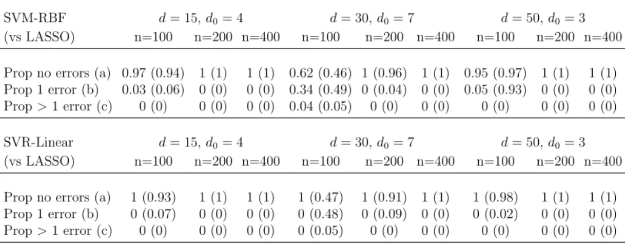
3.10 Simulation Study . . . 68
3.10.1 Consistency and selection of features . . . 68
3.10.2 RFE vs penalized methods . . . 72
3.11 High dimensional framework when pgrows with n . . . 74
3.11.1 Under universal bounds for entropy and approx-imation error . . . 76
3.11.2 Under relaxed bounds for entropy and approxi-mation error . . . 78
3.12 Concluding remarks . . . 79
3.13 Supplementary Materials . . . 80
4 Feature Selection in Q Learning . . . 81
4.1 Reinforcement Learning: Methods and concepts . . . 81
4.1.1 Reinforcement Learning . . . 81
4.1.2 Q Learning . . . 83
4.2 Recursive Feature Elimination . . . 84
4.2.1 The support vector machine algorithm . . . 86
4.3 Feature elimination in Q learning . . . 88
4.4 Methods for feature selection in Q learning . . . 90
4.4.1 Recursive feature elimination on the estimation steps . . . 90
4.4.2 Recursive feature elimination on estimation steps using separate data folds for model training and testing . . . 92
4.4.3 Recursive feature elimination on the final maxi-mization step . . . 94
4.5 Simulation Results . . . 100
4.5.1 Simulation settings . . . 100
4.5.2 Estimation through support vector machines with Gaussian RBF kernel . . . 103
4.5.3 Stopping rule . . . 104
4.5.4 Results . . . 107
4.6 Summary of Chapter 4 . . . 112
4.7 Plots for single runs of the algorithm in some of the settings . . . 113
5 Discussions and Future Projects . . . 122
5.1 Using temporal process regression to study medical adherence . . . 122
5.2 Consistency results for RFE in SVM . . . 125
5.3 Feature selection in Q learning . . . 126
Appendix A: Technical Details for Chapter 2 . . . 128
Appendix B: Technical Details for Chapter 3 . . . 132
B.1 Results for RFE in empirical risk minimization . . . 132
B.1.1 The Recursive Feature Elimination Algorithm for ERM . . . 132
B.1.2 The version of the main result in ERM . . . 132
B.2 Additional materials on RFE . . . 135
B.2.1 A further discussion on Projected Spaces . . . 135
B.2.2 Entropy Numbers . . . 136
B.3 Proofs . . . 137
B.3.1 Proof of Lemma 3 . . . 137
B.3.2 Proof of Lemma 33 . . . 137
B.3.3 Proof of Lemma 8 . . . 139
B.3.4 Proof of Lemma 16 . . . 139
B.3.5 Proof of Proposition 17 . . . 141
B.3.6 Proof of Lemma 20 . . . 143
Appendix C: Technical Details for Chapter 4 . . . 147
C.1 A further discussion on the mechanisms of RFE Vpred . . . 147
LIST OF TABLES
Table
2.1 Final Model P-Values . . . 28
2.2 Viral Load score difference P-Values across Weeks . . . 35
3.1 Accuracy of RFE (vs LASSO) . . . 69
3.2 SVM-wRFE v SVM-woRFE v Lasso v l1 SVM . . . 73
3.3 SVR-wRFE v SVR-woRFE v Lasso . . . 73
4.1 Accuracy of RFE methods in Setting I . . . 105
4.2 Accuracy of RFE methods in Setting II . . . 106
LIST OF FIGURES
2.1 (A) 95% Pointwise Confidence Intervals for effects of adherence (compliance) on the log odds for SVR for the first 24 weeks in separate analyses of the two drugs. (B) 95% Confidence Band for effects of adherence (compliance) on the log odds for SVR
for the first 24 weeks in separate analyses of the two drugs. . . 22 2.2 95% Confidence Band for effects of adherence (compliance) on
the log odds for SVR for the first 24 weeks in separate analyses
of the two drugs smoothed over time. . . 22 2.3 Plots for Hypothesis test T2. . . 26
2.4 Backward Selection Procedure for choosing the significant
covariates in the model. . . 27 2.5 Effect of Race = Caucasian on the log odds for SVR for the
first 24 weeks in separate analyses of the two drugs. . . 28 2.6 Effect of Gender = Male on the log odds for SVR for the
first 24 weeks in separate analyses of the two drugs. . . 29 2.7 Effect of Fibrosis Score on the log odds for SVR for the first
24 weeks in separate analyses of the two drugs. . . 29 2.8 Plot for the main effects and interaction of adherence
(com-pliance) to the drugs on SVR . . . 29 2.9 Plots for the pooled (across weeks) cdf for the two groups
(group 1 consist of patients not adhering to Peginterferon on week 3, while group 2 consist of the remaining patients who did adhere to the drug during that week) for the physical
scores: (A) muscle ache, and (B) irritability. . . 32 2.10 Plots for the pooled (across weeks) cdf for the two groups
(group 1 consist of patients not adhering to Peginterferon on week 3, while group 2 consist of the remaining patients who did adhere to the drug during that week) for the physical
2.11 Plots for the pooled (across weeks) cdf for the two groups (group 1 consist of patients not adhering to Peginterferon on week 3, while group 2 consist of the remaining patients who did adhere to the drug during that week) for the physical
scores: (A) depression, and (B) overall symptom scores. . . 33
2.12 Plots for the pooled (across weeks) cdf for the two groups (group 1 consist of patients not adhering to Peginterferon on week 3, while group 2 consist of the remaining patients who did adhere to the drug during that week) for the phys-iological scores: (A) WBC counts, and (B) NPC counts. . . 34
2.13 Plots for the pooled (across weeks) cdf for the two groups (group 1 consist of patients not adhering to Peginterferon on week 3, while group 2 consist of the remaining patients who did adhere to the drug during that week) for the phys-iological scores: (A) platelet counts, and (B) viral load scores. . . 35
3.1 Reverse Scree Graph for one run of the simulations for (a) SVM with Gaussian Kernel (b) SVR with Linear Kernel with d= 30, d0 = 7 . . . 70
3.2 Linear-Quadratic mixture change point analysis for (a) SVM with Gaussian Kernel for comparable cross validation values of λ and kernel width γ and (b) SVR with Linear Kernel for comparable cross validation values of λ, with d = 30, d0 = 7 for varying sample sizes. The bold dots represent the estimated change points. . . 71
3.3 Linear-Quadratic mixture change point analysis for (a) SVM with Gaussian Kernel for comparable cross validation values of λ and kernel width γ and (b) SVR with Linear Kernel for comparable cross validation values of λ, with d = 50, d0 = 3 for varying sample sizes. The bold dots represent the estimated change points. . . 71
3.4 Stopping rule for the modified algorithm in the limiting design size setting . . . 75
4.1 Steps of Q Learning . . . 83
4.2 Schematics of RFE in nonparametric estimation . . . 86
4.3 Setting I, n= 200, p= 50 . . . 113
4.5 Setting I, n= 400, p= 10 . . . 115
4.6 Setting II, n= 400, p= 50 . . . 116
4.7 Setting II, n= 200, p= 30 . . . 117
4.8 Setting II, n= 800, p= 10 . . . 118
4.9 Setting III, n = 800,p= 50 . . . 119
4.10 Setting III,n = 400,p= 30 . . . 120
CHAPTER 1: INTRODUCTION
Supervised learning deals with the task of inferring a function from labeled training data. When the training data contains the subgroup information and we want to predict the future subgroups, it is a classification problem. And in cases where the training data contains the continuous response values and our aim is to predict future responses, it is a regression problem. In this dissertation we study properties of three of these supervised learning methods and their applicability in clinical studies in depth.
1.1 Temporal Regression and Medical Adherence
Adherence to, or compliance with a medication regimen, is defined as the extent to which patients take medications as prescribed by their health care providers (Osterberg and Blaschke 2005). In recent years, adherence has become a serious area of research in medicine. In this part of the dissertation we use temporal processes to study adherence and its relationship with the medical end-point in the VIRAHEP-C study. Typically information on medical adherence is gathered over time and most of the previous re-search on this topic has failed to incorporate this longitudinal component of adherence in their analysis. This dissertation aims to rectify this and provide an interesting insight into efficient handling of adherence data.
and forty-seven of them, who showed detectable viremia at week 24, were discontinued from the therapy, while the remaining 254 participants with undetectable or indeter-minate HCV RNA by 24 weeks, continued for a total of 48 weeks. Patients attended a baseline visit and then follow-ups at treatment weeks 2,4,8,12 and then monthly up to 48 weeks. In this analysis, however, we only concentrate on the first 24 week window. The endpoint of focus is Sustained Virologic Response (SVR) measured six months post treatment, defined as undetectable viremia (HCV RNA < 50 IU/mL). Details of the VIRAHEP-C protocol can be found at https://www.niddkrepository.org/niddk/ jsp/public/dataset.jsp#VIRAHEP-C. Baseline data included socio-demographic vari-ables (e.g., age, gender, race, marital status, education level, employment status, health insurance status, etc.) and medical variables (e.g., fibrosis level, alcohol consumption, presence of baseline antidepressant use, etc.). The Center for Epidemiologic Studies-Depression (CES-D) (Radloff (1977)) scale was used to measure depression symptoms and a visual analog scale was used to measure symptoms including (i) fatigue, (ii) headache, (iii) muscle aches and pains, (iv) irritability, (v) depression, and an (vi) overall symptom score.
or Ribavirin and did not open the MEMS cap, she/he was considered fully adherent (See Evon et al. (2013) for details).
In analyses involving adherence data, we typically encounter data that are longitu-dinal in nature. For example in the VIRAHEP C study, 401 patients were followed for 24 weeks, and adherence for Peginterferon was recorded once each week, while that for Ribavirin was recorded each day. As observed above, studies on adherence, whether looking at the importance of adherence on medical end-points or analyzing factors that affect adherence in general, mostly involve sample summaries of these longitudinal data. But the drawback of this type of cross-sectional approach is multifold. First of all, it suffers from an immense loss of information, affected by compiling summary statistics pooled over the entire length of the study. Hence hypothesis tests typically proposed to objectify the causal relationships in such analyses are far less powerful. Second of all, by incorporating the temporal nature of adherence, we can observe the covariate effects across the study period which can provide further insight into the dynamic nature of this relationship across time.
The main contribution of this dissertation is providing an insightful approach to analyzing adherence data. In this dissertation, we study the effect of adherence on sustained virologic response, the end point in the VIRAHEP C study, using temporal process regression. Hence in this case, adherence is incorporated as a time-varying covariate in the regression set up and SVR is incorporated as the response and remains constant over time. It is worthwhile to note that a similar approach can be used in reverse studies where adherence is analyzed as the response while looking for mean-ingful factors contributing to varying trends of adherence over time. Another novel contribution of this dissertation is the approach used to create the confidence bands for the processes. In Fine et al. (2004), the authors employ bootstrapping to simulate from the empirical distribution of √n( ˆβ(t)−β0(t)) (the centered covariate effects) to
create confidence bands for β0(t), the true parametric process. In this dissertation we
modify this approach by utilizing the empirical distribution of sup t∈[l,u]
√
to bootstrap from. This method actually helps in establishing a direct relationship between these confidence bands and our proposed hypothesis tests.
1.2 Feature Elimination in Support Vector Machines
In recent years it has become increasingly easy to collect large amounts of infor-mation, especially with respect to the number of explanatory variables or ‘features’. However the additional information provided by each of these features may not be sig-nificant for explaining the phenomenon at hand. Learning the functional connection between the explanatory variables and the response from such high-dimensional data can itself be quite challenging. Moreover some of these explanatory variables or fea-tures may contain redundant or noisy information and this may hamper the quality of learning. One way to overcome this problem is to use variable selection or feature elim-ination techniques to find a smaller set of variables or features that is able to perform the learning task sufficiently well.
the learning, it clarifies the causal relationship in the input-output space, and results in reduced cost of data collection and storage and better computational properties.
One of the earliest works on variable selection in SVM was formulated by Guyon et al. (2002). They developed a backward elimination procedure based on recursive computation of the SVM learning function, known widely as recursive feature elimina-tion (RFE). The RFE algorithm performs a recursive ranking of a given set of features. At each recursive step of the algorithm, it calculates the change in the RKHS norm of the estimated SVM function after deletion of each of the features remaining in the model, and removes the one with the lowest change in such norm, thus performing an implicit ranking of features. A number of modified approaches have been developed since then, inspired by RFE (see Rakotomamonjy 2003, Aksu et al. 2010, Aksu 2012). Alternate wrapper-based selection methods have also been formulated like in Weston et al. (2001), Chapelle et al. (2002). Filters have been used for feature elimination in SVMs in many previous works (see for example Mladenic et al. 2004, Peng et al. 2005). Embedded methods for variable selection include redefining the SVM training to include sparsity (Weston et al. 2003, Chan et al. 2007). For example, Bradley and Mangasarian (1998) suggested the use of the l1 penalty to encourage feature sparsity.
Zhu et al. (2003) suggested an algorithm to compute the solution path for thisl1-norm
SVM efficiently. Other methods include introducing different penalty functions like the SCAD penalty (Zhang et al. 2006), the lq penalty (Liu et al. 2007), a combination of
l0 and l1 penalty (Liu and Wu 2007), the elastic net (Wang et al. 2006), the f∞ norm
(Zou and Yuan 2006), and using a penalty functional in the framework of the smoothing spline ANOVA (Zhang 2006).
functional class for the optimization. Hence the main drawback for these penalized methods (with penalty functions likel1,lq, elastic net, etc.) is that they can only work
in linear kernels, as these become ineffectual concepts in the framework of more complex function classes like RKHSs with non linear kernels. RFE and RFE derived methods however help to address this issue, as these methods can work in complex problems as well, where we might need a larger class of functions (than just the linear space) for the optimization. Another key feature of RFE is that it does feature selection, that is, when a feature is removed, all its effects (main effects and interactions with other fea-tures) are removed. However, the most important drawback for these methods is that arguments for them have mostly been heuristic, and their ability to produce success-ful data-driven performances have been examined only in simulated or observed data. Hence, the theoretical properties of them have never been studied in rigorous detail. A key reason behind this lack of theory is the absence of a well-established framework for building, justifying, and collating the theoretical foundation of such a feature elim-ination method. This part of the dissertation aims at building such a framework and modifying RFE to create a recursive technique that can be validated as a theoretically sound procedure for feature elimination in SVMs.
these spaces remain cognate to one another. The basis for the theory on RFE depends heavily on specifying these pseudo-subspaces, and a contribution of this part of the dissertation is to formulate a way to do this.
Another contribution of this part of the dissertation is a modification of the crite-rion for deletion and ranking of features in Guyon et al.’s RFE to enable theoretical consistency. Here we develop a ranking of the features based on the lowest difference observed in the regularized empirical risk after removing each feature from the exist-ing model. It is important to understand that removexist-ing a feature from the functional model, means not only that the main effect of the feature are removed, but also all complex interactions the feature might have had with the remaining ones in the model, are eliminated as well. The heuristic reasoning behind this is that if any of the features do not contribute to the model at all, the increase in the regularized risk will be incon-sequential. This allows RFE to be generalized to the much broader yet simpler setting of empirical risk minimization where we can apply the same idea to empirical risk. This can thus serve as a useful starting point for the analysis of feature elimination in SVM (details are given in Appendix B.1).
and Chirstmann (2008) (hereafter abbreviated SC08).
The main body of the work is given in Section 3. We present the proposed version of RFE for SVMs, and discuss the concept of feature elimination in this framework. We discuss the assumptions required to establish consistency of RFE in the simpler yet practical settings of nested or dense models. The main consistency results are provided following that, and the implications of these results in some known settings of risk minimization in nested or dense models are discussed in depth, including the setting of risk minimization in linear models and SVM for classification with a Gaussian RBF kernel. Next, we relax the earlier assumptions to allow us to establish consistency of the algorithm in more complex functional spaces. Then we study two more interesting applications of kernel machines in imaging and protein classification and discuss how our method can be useful for feature selection there. Finally, we prove our main result under this most general setting. We provide some simulation results to demonstrate how RFE works and how it can be used in intelligent selection of features, and compare it with penalized methods for feature selection. A general discussion is provided followed by detailed proofs for important results.
1.3 Feature Elimination in Q Learning
Zhao et al. 2014). An ideal treatment rule should be adaptive, robust and tailored to the requirement of a given individual based on his/her prognosis information. With steady advance in treatment methods and a better understanding of human genetics, researchers have been able to incorporate this new information into clinical diagno-sis. Research projects into human genetics have paved way for better understanding of genes in an individual’s physiology and development. Researchers have now been able to discern the role of single nucleotide polymorphisms (SNPs), that account for genetic variabilities between individuals and as a result genome-wide association stud-ies (GWAS) have been conducted to examine genetic variation and risk for common diseases.
2010).
often impractical to obtain examples of desired behavior that are both correct and representative of all the situations in which the agent has to act. In uncharted territory where one would expect learning to be most beneficial an agent must be able to learn from its own experience.
Finding therapies tailored to each individual in settings involving multiple decision times is a major challenge, and Q-learning can be used for maximizing the average sur-vival time of patients as a function of prognostic factors, past treatment decisions, and optimal timing. Zhao et al. (2009) introduced the clinical reinforcement trial concept based on Q-learning for discovering effective therapeutic regimens in potentially irre-versible diseases such as cancer. The concept is an extension and melding of dynamic treatment regimes in counter factual frameworks (Murphy 2003, Robins 2004) and se-quential multiple assignment randomized trials (Murphy 2005a) to accommodate an ir-reversible disease state with a possible continuum of treatment options. This treatment approach falls under the general category of personalized medicine. The generic cancer application developed in Zhao et al. (2009) takes into account a drugs efficacy and toxicity simultaneously. The authors demonstrate that reinforcement learning method-ology not only captures the optimal individualized therapies successfully, but is also able to improve longer-term outcomes by considering delayed effects of treatment.
multifold. We can incur serious cost in collection and storage of this information but more importantly, this increases significantly the chances of overfitting. In presence of high-dimensional information, it is possible then that the Q-functions are poorly fitted or even grossly overfitted, and an overfitted model is not generalizable for predicting optimal treatments for future patients. In presence of noise or misspecification of the models for the Q functions, the fitted Q-functions may not necessarily result in maximal long-term clinical benefit. Like in any other learning problem, overfitting is an issue that needs to be addressed, and hence feature elimination is of significant importance in reinforcement learning frameworks and this is the primary focus for this part of the dissertation.
to study three such methods for feature selection in Q learning. The idea stems from our earlier work (see Dasgupta et al. 2013), where we studied a backward feature selec-tion method called the recursive feature eliminaselec-tion in support vector machines, and showed its generability in a variety of complex settings, when standard methods fail. We even showed that under certain regularity conditions, the method we proposed is consistent in finding the correct subset of features in these situations, thus establishing the usefulness of such a method in this regard.
The third method differ significantly from the first two methods, but in essence is a backward selection method as well. Two important differences include,
(1) Unlike the first two methods, this method works on the entire model building procedure, and not sequentially on each estimation phase.
(2) The model evaluation criterion is not regularized risk, but the optimal value function itself.
At each step of the feature selection procedure here, given the current size of the histories (H1, . . . , HT), we train the entire Q learning algorithm to obtain the empirical estimates of the stage 1 value function on submodels created sequentially by removing one feature at a time from the cumulative history, and then choosing the one that produces the highest estimate of the stage 1 value function for deletion. Heuristically this makes sense, as one of the main goals of the Q learning algorithm is to maximize the optimal stage 1 reward or value function.
1.4 Overview of the dissertation
CHAPTER 2: USING TEMPORAL REGRESSION TO STUDY ADHERENCE IN HEPATITIS C
2.1 Methods
In this section we review temporal process regression. We start off with a brief review of the model and assumptions, and explain how to produce pointwise confidence intervals and confidence bands for the processes. We also discuss how to use smooth-ing to getter better estimators of these processes and their confidence bands. Lastly we propose some hypothesis tests to test for the significance of the effects of these parametric processes in the given framework.
2.1.1 Model
Fine et al. (2004) proposed the following functional generalized linear model as an extension of standard linear models. The mean of the response Y(t) at time t is specified conditionally on ap×1 vector of time-dependent covariates X(t). That is,
µ(t) =E(Y(t)|X(t)) = g−1{β(t)0X(t)} (2.1)
where the link function g is monotone, differentiable, and invertible, and β(t) =
{β1(t), . . . , βp(t)} is a p×1 vector of time-dependent coefficients. The parameterβ(t) has a clear meaning in the model at time t and because the link is time-independent,
β(s) and β(t) are comparable fors6=t.
whether that patient attained SVR at the end of the study. Xi(t) is the covariate vector for patient i at time t (which includes adherence) and the link function is given as g−1 = exp/(1 + exp). Hence this actually gives us a time-indexed logistic model
with β(t) denoting the change in the log odds ratios for SVR per unit increase in the covariates at time t. Hence this can be interpreted as a cluster of generalized linear models, one for each time pointt. We obtain estimates for the changes in the log odds ratios for SVR for different covariates for each time point t and these estimated effect sizes can be interpreted as processes varying over time. In practice, the data processes may be missing at some times. We only take into consideration those time points t
where{Y(t), X(t)} is fully observed at t.
Within a time interval [l, u], we continuously observen independent and identically distributed copies of {Y(t), X(t) : R(t) = 1}, where Y is the response, X is a p×1 covariate vector, and R is the data availability indicator, which permits both missing response and missing covariates. The estimator for β(t) may be computed separately at each t. Denote ˆβ(t) as the root of U{β(t), t}=
n
X
i=1
Ai(β(t), t), where
Ai{β(t), t}=Ri(t)D0i{β(t)}Vi{β(t), t}[Yi(t)−µi(t)}]
Di0{β(t)}=∂[g−1{β(t)0X
i(t)}]/∂{β(t)} andVi{β(t), t}is a weight matrix possibly ran-dom.
The estimator potentially jumps at those M times where {Yi(t), Xi(t) : Ri(t) = 1} and Ri(t) jumps. Let j1 < · · · < jM be the jump points. Finding ˆβ(t) involves solvingU{β(t), t}at the M points. According to Fine et al. (2004), in theory, when the processes vary between ji, smoothing is not required. But in practice, the equations are solved on a grid and the estimators are interpolated via smoothing. If Yi(t) and
2.1.2 Pointwise Confidence Intervals
Under appropriate conditions (See Liang and Zeger (1986)), for each t, ˆβ(t) is consistent for β0(t), the true value of β(t) and for any K < ∞ points with l < t1 < · · ·< tK < u,n1/2[{βˆ(t1)0, . . . ,βˆ0(tK)}0−{β0(t1)0, . . . , β0(tK)0}] is asymptotically normal with covariance consistently estimated by the sandwich estimator.
Hence pointwise confidence intervals forβ0(t) may be constructed using the normal
approximation and the sandwich variance estimate
ˆ
Σ(t, t) ={Hˆ(t)−1}Gˆ(t, t){Hˆ(t)−1}0,
where ˆH(t) and ˆG(t, s) are given by
ˆ
H(t) =n−1
n
X
i=1
Ri(t)D0i{βˆ(t)}Vi{βˆ(t), t}Di{βˆ(t)},
ˆ
G(s, t) = n−1
n
X
i=1
Ai{βˆ(s), s}Ai{βˆ(t), t}0.
A 100(1−α)% confidence interval at time t for βk0(t) is ˆβk(t)±n−1/2zα/2Σˆk(t, t)1/2 where zα/2 is the (1−α/2) percentile of the standard normal distribution and ˆΣk(t, t) is the kth diagonal element of ˆΣ(t, t).
2.1.3 Confidence Bands
In Fine et al. (2004), the authors show that the consistency and weak convergence results hold uniformly in t, that is, ˆβ(t) converges uniformly to β0(t) for t ∈ [l, u]
and n1/2{βˆ(t)−β
0(t)} converges weakly to a tight zero mean Gaussian process G(·)
with continuous sample paths at continuity points ofβ0(t) with the covariance function
Σ(s, t) = hn1/2{βˆ(t)−β
0(t)}, n1/2{βˆ(t)−β0(t)}
i
= {H(s)−1}G(s, t){H(t)−1}0, where
However, constructing confidence bands forβ(t) for t∈[l, u] is analytically difficult since the Gaussian process G(·) does not have a canonical representation. Instead, we can employ resampling, either by bootstrapping the empirical data distribution and solving U{β(t), t} repeatedly, or by simulating directly from the process, as in Lin, Fleming, and Wei (1994). For a better understanding of this, one may refer to Chap-ter 22, Section 3 of Kosorok (2008) which studies this particular case in detail. In this analysis we however use a conservative approach. We sample from the empirical distribution of a standardized version of supt|βˆ(t)−β0(t)|. This results in wider
con-fidence bands. The importance of this approach lies in the fact that we can obtain a direct correspondence between these confidence bands and hypotheses tests which will be explained later. The way we generate these confidence bands is as follows:
We use the fact that n1/2{βˆ(t)−β
0(t)}=n−1/2
Pn
i=1ψi(t) +o
t
p(1) where
ψi(t) ={H(t)}−1Ai{β0(t), t}
is the influence function for the process ˆβ(t). Note that the sandwich variance estimator is given by ˆΣ(s, t) as before. Now we can defineψˆi(t) as
ˆ
ψi(t) = [diag( ˆΣ(t, t))]−1/2{Hˆ(t)}−1Ai{βˆ(t), t}.
Hence we can create 100(1−α)% simultaneous confidence bands of the form
ˆ
βk(t)±n−1/2bk,α/2Σˆk(t, t)1/2, (2.2)
wherebk,α/2 is the (1−α/2)-th quantile of the empirical distribution of thekth
compo-nent ofBn where,
Bn= sup t
n
n−1/2
n
X
i=1
ziψˆi(t)
from repeatedly samplingz1, . . . , zn ∼ i.i.d. N(0,1).
2.1.4 Smoothing the estimated parametric function
Smoothing is a class of regression techniques to estimate a real valued functionf(X) over the domain R by using its noisy observations, and fitting a different but simple model separately at each query point x0. This is done by using observations close to
the target pointx0 to fit the simple model, in such a way that the resulting estimated
function is smooth in R.
Here we assign weights that die off smoothly with distance from the target point. For each t0, the Nadaraya-Watson kernel-weighted average is defined as
˜ ˆ
β(t0) =
Pn
i=1Kλ(t0, ti) ˆβ(ti)
Pn
i=1Kλ(t0, ti)
.
We use the triangular kernel for smoothing, defined as
Kλ(t0, t) = D
|t0−t| λ
,
where
D(t) = (1−t) if|t|<1 = 0 otherwise
The amount of smoothing that we want can be controlled by the kernel widthλ, where
(A)
(B)
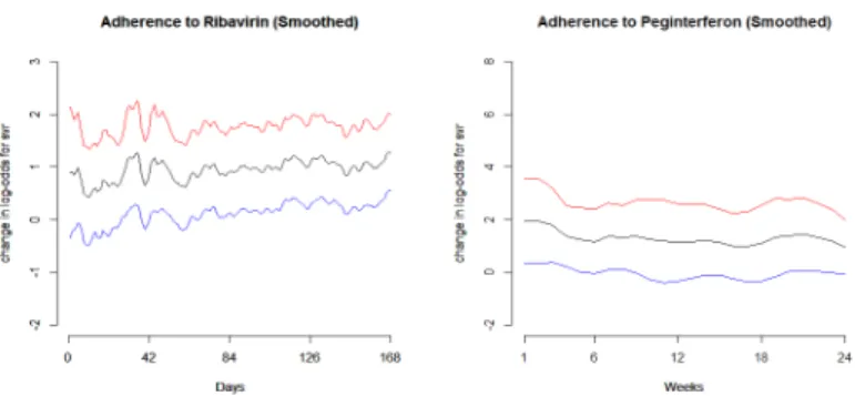
Figure 2.1: (A) 95% Pointwise Confidence Intervals for effects of adherence (compliance) on the log odds for SVR for the first 24 weeks in separate analyses of the two drugs. (B) 95% Confidence Band for effects of adherence (compliance) on the log odds for SVR for the first 24 weeks in separate analyses of the two drugs.
Figure 2.2: 95% Confidence Band for effects of adherence (compliance) on the log odds for SVR for the first 24 weeks in separate analyses of the two drugs smoothed over time.
2.1.5 Confidence bands using the smoothed estimators
We have
n1/2{βˆ(t)−β0(t)}=n−1/2
n
X
i=1
ψi(t) +otp(1),
where ψi(t) is defined as before. Now if ˆψi(t) is the estimated influence function, then define ψ˜ˆi(t) to be the smoothed version of ˆψi(t). Hence we can produce smoothed version of the Sandwich variance estimator asΣ(˜ˆ t, t) = n−1Pn
i=1
h˜
ˆ
ψi(t)
i h˜
ˆ
ψi(t)
i0
. Now define ψ˜ˆi(t) as ψ˜ˆi(t) = [diagΣ(˜ˆ t, t)]−1/2ψ˜ˆ
i(t), and hence we can create 100(1− α)% smoothed simultaneous confidence bands of the form
˜ ˆ
βk(t)±n−1/2˜bk,α/2Σ˜ˆk(t, t)1/2,
where ˜bk,α/2 is the (1−α/2)-th quantile of the empirical distribution of thekth
compo-nent of ˜Bn where,
˜
Bn= sup t
n
n−1/2
n X i=1 zi ˜ ˆ
ψi(t)
o
from repeatedly sampling z1, . . . , zn ∼ i.i.d. N(0,1). This follows from the continuous mapping theorem.
2.1.6 Non-parametric hypothesis tests
Fine et al. (2004) proposed three different non parametric tests for testing the null hypothesis H0 : C(t)β(t) = c(t), where at each t, C(t) is an r× p contrast matrix
and c(t) is an r×1 vector of constants. This general framework allows global tests for multiple hypotheses. In this analysis, we consider only two of them. The first statistic is an integrated difference statistic (IDS). DefiningM(t) :=C(t) ˆβ(t)−c(t) we have,
T1 = ˆ u
l
where W is a non-negative weight function, possibly random. Under mild conditions
T10Σˆ−11T1 is asymptotically χ2r under H0, where
ˆ
Σ1 =n−2
n
X
i=1
ˆ u l
C(s) ˆH(s)−1Ai{βˆ(s), s}W(s)ds
⊗2
,
and for a vectorv, v⊗2 =vv0. The second statistic is the supremum difference statistic
(SDS), based on the sup-norm distance,
T2= sup
t∈[l,u]
M(t)0
n
C(t) ˆΣ(t, t)C(t)
o−1
M(t)
.
Similarly to most Kolmogorov-Smirnov type statistics, the distribution of T2 is rather
complex and is typically approximated by resampling.
A simple test of βj = 0 can be visually determined by looking at the confidence band of βj and determining whether at any time point the whole portion of the band lies above or below 0.
2.2 Results
conclusions.
2.2.1 Initial Plots
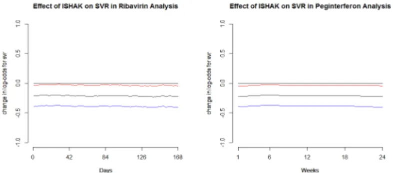
We begin by using temporal process regression to model Ribavirin and Peginterferon separately. Figure 2.1(A) shows the estimated effect sizes for adherence on SVR in the two analyses. Hence for the Ribavirin analysis, the estimated effect size β(t) for the tth day (as seen in the plot) is the log odds for an individual under complete compliance with Ribavirin on the tth day, to attain SVR over an individual under partial or no compliance with the drug on that day. Similarly for the Peginterferon analysis, the estimated effect size for the ith week is the log odds for an individual under compliance with Peginterferon on theith week, to attain SVR over an individual under no compliance with the drug during that week. In Figure 2.1(A), we also plot the 95% pointwise confidence intervals for these processes. Figure 2.1(B) is a plot of the 95% confidence bands for the change in log odds for SVR under complete compliance for the two drugs. As expected, the confidence bands are wider than pointwise confidence intervals.
As is evident from Figures 2.1(A) and 2.1(B), the estimated processes are quite noisy, since we estimate the effects on a daily or a weekly grid (depending on the drug we are analyzing) and interpolate over rest of the interval. Hence to obtain a better estimate of the processes, we employ kernel smoothing (refer to Section 2.1.4). The results are presented in Figure 2.2. We provide the estimated processes smoothed over time along with their 95% confidence bands.
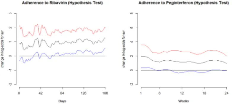
2.2.2 Results of Non Parametric Hypothesis Tests
Results for T1 (IDS): Separately, adherence to Ribavirin (p = 8.413 ×10⁻⁷) and
by the integrated difference statistic.
Results for T2 (SDS): As we see in Figure 2.2(D), the lower confidence bands cross 0
indicating that the effects are found to be positively significant for both Ribavirin and Peginterferon by the supremum difference statistic.
Figure 2.3: Plots for Hypothesis test T2.
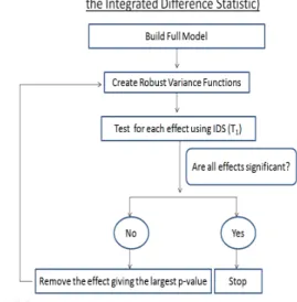
2.2.3 Backward Selection of Covariates
We fit a full model considering other predictors, and follow a gradual step down procedure to remove the ones which weren’t found to be significantly associated with SVR, after controlling for the other predictors. The covariates considered for the full model are listed below:
• SEX : Gender
• RACEW: Whether caucasian/african-american • MXAD: History of anti-depressant use
• Age: Age of the subject
• ISHAK: Indicator of severity of disease (fibrosis score)
• Education: Education level of the subject • Insurance: Insurance provider for the subject • Employ: Employment Status
• Marital: Marital Staus • Alcohol: Alcoholic Status
• Vload: Baseline Viral Load Score
A flow chart of the Backward Selection procedure is given in Figure 2.4. The steps are performed for analyses of both drugs. The final models after the step down process
Figure 2.4: Backward Selection Procedure for choosing the significant covariates in the model.
are found to consist of the same covariates and are shown in Table 2.1.
2.2.4 Plots for other significant covariates
Covariates Ribavirin Analysis Peginterferon Analysis
SEX 0.029 0.016
RACE 4.71e-05 2.81e-05
ISHAK 0.009 0.009
Table 2.1: Final Model P-Values
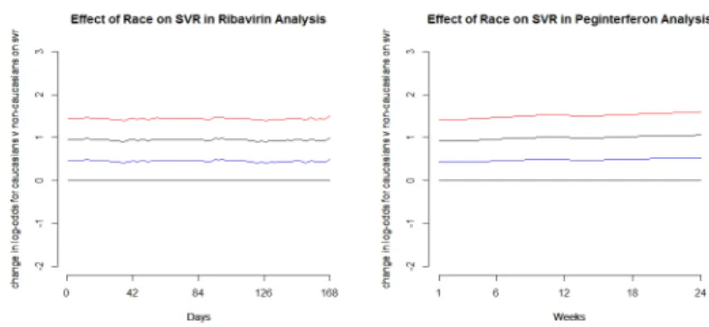
Figure 2.5: Effect of Race = Caucasian on the log odds for SVR for the first 24 weeks in separate analyses of the two drugs.
adherence, SEX, RACEW and ISHAK are significantly associated with SVR too. We plot the estimated effects in Figures 2.5–2.7.
Figure 2.6: Effect of Gender = Male on the log odds for SVR for the first 24 weeks in separate analyses of the two drugs.
Figure 2.7: Effect of Fibrosis Score on the log odds for SVR for the first 24 weeks in separate analyses of the two drugs.
2.2.5 Combined Analysis
Since the prescribed regimen is really a combination of the two drugs, we now conduct an analysis on the combined Ribavirin-Peginterferon data. We first incorporate only the fixed effects for adherence to the drugs (Peginterferon and Ribavirin) and the covariates (SEX, RACEW and ISHAK) found significant in the separate analyses. Since Peginterferon is taken once every week, the analysis is done across weeks. The daily information on the Ribavirin drug is introduced as a score vector of length 7 for each week, with theithelement recording the score forithday of the week (i= 1, . . . ,7). The first hypothesis that we test is H0 : β1 = · · · =β7, where the parameter βi represents the effect of adherence to Ribavirin on SVR for theith day of the week. Hence we test whether the effect of adherence to drug Ribavirin on SVR is the same across different days of a week. Both the Integrated Effect Test T1 (p = 0.863) and the Supremum
Effect TestT2(p = 0.561) showed lack of sufficient evidence against the null hypothesis,
meaning that the Ribavirin adherence can be adequately summarized by the weekly average.
Accordingly, we now create a single covariate for adherence to Ribavirin for each week by taking the average of the daily scores for each week. We then test for the signif-icance of adherence to the drugs in the same model. The integrated difference statistic shows that the individual effects of the drugs Ribavirin (p = 0.0202) and Peginterferon (p = 0.009) are still both significant, though the more conservative supremum differ-ence statistic did not find sufficient eviddiffer-ence at 5% level of cut-off to support that (p 0.258 and 0.081 for Ribavirin and Peginterferon respectively). However both tests, IDS and SDS found the joint effect of the drugs to be highly significant (p = 0.00026 and 0.007 respectively).
change of log odds for SVR). We make a very interesting observation from the analysis as seen in Figure 2.8, where we see huge peaks in the estimated main effects of adher-ence for the two drugs, and a huge dip in the estimated interaction effect on week 3. On further investigation of SVR on week 3, we realize that there is a perfect separation of the data based on the interaction of the two drugs Ribavirin and Peginterferon. All of the subjects who were non-adherent to Peginterferon for that week and were at best partially adherent to Ribavirin for the whole week, didn’t show Sustained Virologic Response at the end of the study. Also interestingly, only 1 among 22 patients (4.55%) who were non-adherent to Peginterferon for that week showed Sustained Virologic Re-sponse at the end of the study, while the percentage of SVR among those who did adhere to Peginterferon on week 3 was 41.11%. This calls for further analysis on these 22 patients who failed to adhere to the drug Peginterferon on week 3.
2.2.6 Diagnostic analysis
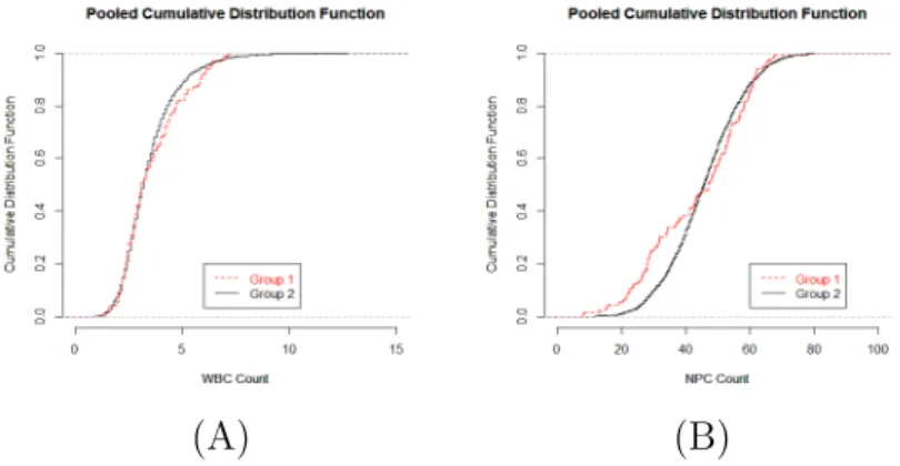
On week 3, 22 patients did not adhere to Peginterferon (group 1) while the remaining individuals did (group 2) adhere to Peginterferon. We want to compare these two groups with respect to several criterion scores, both physical and physiological. The physical scores include various symptom scores, (i) Muscle Ache, (ii) Irritability, (iii) Headache, (iv) Fatigue, (v) Depression, and (vi) Overall. And the physiological scores include various internal measurements such as, (i) WBC count, (ii) NPC count, (iii) Platelet count, and (iv) Viral Load scores.
In Figures 2.9 – 2.13, we look at the cumulative distribution plots of these scores, pooled across the entire length of study.
(A) (B)
Figure 2.9: Plots for the pooled (across weeks) cdf for the two groups (group 1 consist of patients not adhering to Peginterferon on week 3, while group 2 consist of the remaining patients who did adhere to the drug during that week) for the physical scores: (A) muscle ache, and (B) irritability.
(A) (B)
Figure 2.10: Plots for the pooled (across weeks) cdf for the two groups (group 1 consist of patients not adhering to Peginterferon on week 3, while group 2 consist of the re-maining patients who did adhere to the drug during that week) for the physical scores: (A) headache, and (B) fatigue.
(A) (B)
Figure 2.11: Plots for the pooled (across weeks) cdf for the two groups (group 1 consist of patients not adhering to Peginterferon on week 3, while group 2 consist of the re-maining patients who did adhere to the drug during that week) for the physical scores: (A) depression, and (B) overall symptom scores.
except the viral load scores. A 5000 simulation run gave a p. value of 0.0094, demon-strating that the distribution of the pooled viral load scores for the two groups are significantly different. Viral Load scores being a response criterion for our study indi-cates that early adherence to Peginterferon is extremely important. In Table 2.2, we give results from the Cramer von Mises test on the difference in viral load scores be-tween the two groups on individual readings. The Cramer von Mises criterion showed non-significant results for the initial two time points. At the 3rd time point (week 2) it approaches statistical significance and is significant by week 4.
2.3 Summary of Chapter 2
(A) (B)
Figure 2.12: Plots for the pooled (across weeks) cdf for the two groups (group 1 con-sist of patients not adhering to Peginterferon on week 3, while group 2 concon-sist of the remaining patients who did adhere to the drug during that week) for the physiological scores: (A) WBC counts, and (B) NPC counts.
(A) (B)
Figure 2.13: Plots for the pooled (across weeks) cdf for the two groups (group 1 con-sist of patients not adhering to Peginterferon on week 3, while group 2 concon-sist of the remaining patients who did adhere to the drug during that week) for the physiological scores: (A) platelet counts, and (B) viral load scores.
Vload Score Reading Cramer V Mises P-value
Day 1 0.2765
Week 1 0.2208
Week 2 0.0769
Week 4 0.0030
Week 8 0.0833
Week 12 0.1932
CHAPTER 3: CONSISTENCY RESULTS FOR RECURSIVE FEATURE ELIMINATION IN SVM
3.1 Preliminaries
We begin by introducing some notations and discussing support vector machines (and empirical risk minimization as a related concept).
Let the input space (X,A) be measurable, such that X ⊆ B ⊂Rd, where B is an open Euclidean ball centered at 0. LetY be a closed subset ofRandP be a measure on
X × Y. A function L:X × Y ×R7→ [0,∞] is called a loss function if it is measurable. We say that a loss function is convex ifL(x, y,·) is convex for every x∈ X and y∈ Y. A loss function is called locally Lipschitz continuous with Lipschitz local constantcL(·) if for every a >0,
sup x∈X,y∈Y
|L(x, y, s)−L(x, y,´s)|< cL(a)|s−s|´ , s,s´∈[−a, a].
L is said to be Lipschitz continuous if there is a constant cL such that cL(a) ≤ cL
∀a∈R.
For any measurable function f : X 7→ R, we define the L-risk of f with respect to the measure P as RL,P(f) = EP[L(X, Y, f(X)]. The Bayes Risk R∗L,P is defined as inffRL,P(f), where the infimum is taken over the set of all measurable functions,
Let F ⊆ L0(X) be a non-empty functional space, andL be any loss function. Let
fP,F = arg min
f∈F
EP[L(X, Y, f(X)] = arg min f∈F
RL,P(f) (3.1)
be the minimizer of infinite-sample risk within the space F. We define the minimal risk within the space F as R∗
L,P,F = RL,P(fP,F). The empirical risk is denoted by
RL,D (where the subscriptD denotes the empirical measure invoked by the data D =
{(X1, Y1), . . . ,(Xn, Yn)} ∈ (X × Y)n), and is given as, RL,D(f) ≡Pn(L(X, Y, f(X)) = 1
n
n
X
i=1
L(Xi, Yi, f(Xi)).
Empirical Risk Minimization: A learning method whose decision functionfD,F
minimizes empirical risk RL,D(f) among the class of functions {f : f ∈ F }, for all
n ≥1 and data D is called empirical risk minimization (ERM) with respect to L and
F.
Now let H be an R-Hilbert space over X. A function k : X × X 7→ R is called a reproducing kernel of H if k(·, x) ∈ H for all x ∈ X, and has the reproducing property f(x) = hf, k(·, x)i for all f ∈ H, and all c ∈ X. The space is called a real-valued Reproducing Kernel Hilbert Space (RKHS) over X (For a better understanding of RKHSs, we refer our readers to SC08).
Support Vector Machines: LetH be a separable RKHS of a measurable kernel
k onX, and fix a λ > 0. Let L be convex and locally Lipschitz continuous. Then the empirical SVM decision function can be defined as,
fD,λ,H = arg min f∈H
λkfk2H +RL,D(f). (3.2)
For a given λ, the SVM learning method L is the map (X × Y)n× X 7→R defined by (D, x) 7→ fD,λ,H(x) for all n ≥ 1. Like before, we can define the infinite sampled version of the regularized minimizer as fP,λ,H = arg min
f∈H
approximation error is given by,
AH2 (λ) = λkfP,λ,Hk2H +RL,P(fP,λ,H)− inf
f∈HRL,P(f). (3.3)
Note: The results developed in this paper are valid not only for classification,
but also for regression under certain general assumptions on the output space Y. For simplicity however, we will refer to both these variants in this paper as SVM, unless otherwise mentioned.
3.2 Feature Elimination Algorithm
The original recursive feature elimination (RFE) algorithm was proposed for SVMs by Guyon et al. (2002), the performance of which was evaluated under experimental settings. Limitations of this method as a margin-maximizing feature elimination was studied explicitly in Aksu et al. (2010). The version proposed here is similar in structure to Guyon et al., but differ in the elimination criterion. While Guyon et al. used the Hilbert space normλkfk2
H to eliminate features recursively, we use the entire objective function (the regularized empirical risk) for deletion.
3.2.1 The Algorithm
We begin by proposing a way such that starting off with a space F, we are able to create lower dimensional versions of it. As mentioned before, this is indeed necessary, since at each stage of the feature elimination process, we move down to a ‘lower di-mensional’ feature space and the functional spaces need to be adjusted to cater to the appropriate version of the problem in these subspaces. A detailed discussion on these will be given in Section 3.3.
defineFJ ={g :g =f◦πJc ,∀f ∈ F }, where πJc is the projection map from x 7→xJ
(x, xJ ∈ Rd), such that xJ is produced from x by replacing those elements in x which are indexed in the set J, by zero.
We can hence define the space XJ ={πJc
(x) : x∈ X }, such that πJc
:X 7→ XJ is a surjection. Now we are ready to provide the algorithm. Assume the support vector machine framework, where we are given an RKHSH indexed by a kernel k.
Algorithm 2. Start off with J ≡[·] empty and let Z ≡[1,2, ..., d].
STEP 1: In the kth cycle of the algorithm choose dimension ik for which
ik =arg min i∈Z\J
λfD,λ,HJ∪{i}
2
HJ∪{i}+RL,D fD,λ,HJ∪{i}
−λfD,λ,HJ
2
HJ − RL,D fD,λ,HJ
. (3.4)
STEP 2: Update J =J ∪ {ik}. Go to STEP 1. Continue this until the difference
min i∈Z\Jλ
fD,λ,HJ∪{i}
2
HJ∪{i}+RL,D fD,λ,HJ∪{i}
−λfD,λ,HJ
2
HJ−RL,D fD,λ,HJ
becomes
larger than a pre-determined quantity δn, and output J as the set of indices for the features to be removed from the model.
See Appendix B.1.1 for a version of the algorithm for empirical risk minimization problems.
3.2.2 Cycle of RFE
runs of the algorithm the cycle sizes are different. The theoretical results derived in this paper will hold for cycles of any size. Here for the sake of simplicity, we set the cycle size to 1.
3.3 Functional Spaces on Lower Dimensional Domains
The aim of this section is to provide a detailed reasoning behind Definition 1 in Section 3.2.1.
3.3.1 Feature Elimination in SVM
In empirical risk minimization problems our primary focus is empirical riskRL,D(f), while in support vector machines our main concern is the regularized version of this risk, λkfk2
F +RL,D(f). The minimization in case of SVMs is typically computed over special functional classes called RKHSs (denoted by H here). Our objective is then to find fD,λ,H ≡ arg min
f∈H
λkfk2
H +RL,D(f). The regularization term λkfk2H is used to penalize functions f with a large RKHS norm. Complex functionsf ∈H which model the output values in the training data set D too closely, tend to have larger H-norms (Refer to Exercise 6.7 in SC08 for a clear motivation).
Now consider the setting of empirical risk minimization in general (and SVM as a special case). Consider L∞(X), the space of all bounded measurable functions from
X 7→Rand suppose we start off with a functional classF ⊆ L∞(X)1 (or,H⊆ L∞(X)),
where X is as defined in Section 3.1. Let our goal be to find a function f within F
(or withinH) that minimizes the given empirical criterion, empirical risk in ERMs (or regularized risk in SVMs). Now if the dimension d of the input space is too large, it might lead to solutions that are too complex than what is sufficient for our purpose.
1Note that the loss functions we consider in this paper (unless otherwise mentioned) are convex
and locally Lipschitz withRL,P(0)<∞, and hence by (2.11) and Proposition 5.27 of SC08, we have
R∗
L,P,L∞(X)=R
∗
Suppose now that the minimizer of infinite-sampled risk with respect to the oracle measure P and the functional class L∞(X), actually resides in L∞(X∗), where X∗ is
a lower dimensional version of X. Then it may actually suffice to find the empirical minimizer in a suitably defined lower dimensional version of F (or the RKHS H), and to avoid overfitting it might become a necessity. The need for defining the lower dimensional adaptations of a given arbitrary functional class (or a given RKHS) in the way of Definition 1 arises from this observation itself. Now the motivation for our algorithm stems from the heuristic belief that if some of the covariates are unimportant or superfluous for the problem at hand, the contribution of each of these variables in the functional relationship between the output variable and the covariate space in terms of the solution might be small at best, that is the incremental risk associated with a solution defined on a subset of the covariate space (by ignoring these surplus variables), when compared to the solution in the original covariate space, might indeed be minimal.
3.3.2 Further discussions on the lower dimensional spaces FJ (or HJ) First note that for a given input spaceX,XJ may not be a subspace of X. However the assertion holds trivially for any Euclidean open ballB centered at 0. So we assume that X ⊆B ⊂Rd. We will also assume that we can sufficiently extend F(X) to F(B) (or, HX toHB when H is a RKHS), such that the domain of functions in F(B) (or in the RKHS HB) is B instead of X. In case of the RKHS H, this in turn extends the domain of the kernelk fromX × X toB×B. Hence from here onwards we will assume
We now provide a few results that connect these lower dimensional spaces with the original one. In view of Definition 1, we can define LJ
∞(X) ={f◦πJ
c
: f ∈ L∞(X)}.
Then Lemma 3 below says that LJ
∞(XJ) ≡ LJ∞(X)
XJ is isomorphic to the space
L∞(XJ). Lemma 4 below, observes some results connecting the original RKHS with
its lower dimensional versions. A related lemma, Lemma 33 is given in Appendix B.1 noting similar results for any general space. These aim to show that many of the nice properties of a given functional space are carried forward to their re-adaptations under Definition 1. We prove Lemma 3 and 33, while proof for Lemma 4 is omitted as it follows from Lemma 33 trivially. The proofs can be found in Appendix B.3.1 and B.3.2 respectively.
Lemma 3. LJ
∞(XJ) = L∞(XJ).
Lemma 4. Let H ⊂ L∞(X) be a non-empty RKHS on X. Then for any J ⊂
{1,2, . . . , d},
1. If H is dense in L∞(X), then HJ is dense in L∞(XJ).
2. If the k · k∞ closure BH of the unit ball BH is compact, then so is BHJ.
3. If H is separable, then so is HJ.
4. ei(id : HJ 7→ L∞(X)) ≤ ei(id : H 7→ L∞(X)), where ei(id : H 7→ L∞(X)) is
the ith entropy number of the unit ball B
H of the RKHS H, with respect to the
k · k∞-norm (see Appendix B.2.2 for a definition of entropy numbers).
3.3.3 RKHS in lower dimensions
that effect, we begin this section by providing an alternate way to define the lower dimensional versions of a given RKHS that preserves the reproducing property.
Definition 5. For a given RKHS H indexed by a kernel k and a set of indices J ⊆ {1,2, .., d}, define HJ ≡H
k◦πJ c(X), where k◦πJ c
(x, y) :=k(πJc
(x), πJc (y)).
Note immediately that Definition 5 allows us to create lower dimensional versions of an RKHSH in a way which ensures that these spaces are RKHS as well. This inevitably questions the validity of Definition 1. We however show below that both Definitions 1 and 5 actually yield the same RKHS space HJ. We begin with the following result due to Paulsen (2009).
Proposition 6. Let S be any set and ϕ:S 7→ X be a map. Letk :X × X 7→R be the kernel on X. If we define the map k◦ϕ : S × S 7→ R as, k ◦ϕ(s, t) = k(ϕ(s), ϕ(t)), then k◦ϕ is a kernel on S. (Paulsen 2009, Proposition 5.13).
The next theorem then gives a natural relationship between RKHSsH(k) onX and
H(k◦ϕ) on S. It also implies that when S is a subset of X and ϕ is the inclusion id
map of S intoX, the kernel k◦ϕ becomes the restriction of the kernel k on S × S. Theorem 7. Let X and S be two sets and let k :X × X 7→R be a kernel function on
X and let ϕ : S 7→ X be a function. Then H(k ◦ϕ) = {f ◦ϕ : f ∈ H(k)}, and for
g ∈H(k◦ϕ) we have that kgkH(k◦ϕ)= inf{kfkH(k) : g =f ◦ϕ}.
See Paulsen (2009) for a proof of Theorem 7.
Now letX0 be a subset ofX andk(0)(x, y) be the restriction of a kernelkonX0. Let Hk(X) be the RKHS with respect to k(x, y), and Hk(0)(X) be the one with respect to
k(0)(x, y). Then by the above theorem, if we defineϕto be the inclusion id map fromX 0
toX, we have Hk(0)(X0) ={f|X0 :f ∈Hk(X)}and kgkHk(0) = min{kfkHk : f|X0 =g}
Taking X0 ≡ XJ and k(0)(x, y) ≡ k(πJ
c
(x), πJc(y)), we immediately obtain our assertion.
3.3.4 Notion of risk in Lower Dimensional Versions of the Input Space Note that the functional spaceFJ (and equivalently RKHSHJ) is defined on the en-tire input spaceX and not only onXJ. So we can define risk for a functionf
J ∈ FJ (or
fJ ∈HJ) for the entire input spaceX and not just forXJ. Hence for a probability dis-tribution P on X × Y, defineRL,P(fJ) as RL,P(fJ) =
´
Y
´
X L(y, x, fJ(x))P(x, y)dxdy.
This allows us to compare the risk of functions in different lower dimensional versions of the original functional space.
3.4 RFE in nested or dense models
In this section we discuss the consistency of our feature elimination algorithm (for both ERM and SVM), when the functional space considered for the problem admits nice properties, like nestedness or denseness. We begin this section by defining these properties and citing important situations when we encounter these spaces. We then discuss our inherent assumption for existence of a null model in these frameworks, and show how that translates to the idea of variable selection through our backward elimination algorithm.
3.4.1 Nested spaces in risk minimization
Often in risk minimization, the space of functionsF we consider for optimization will admit the nested property. To explain it mathematically, for a pairJ1, J2 ∈ {1,2, . . . , d}
with J1 ⊆ J2, the subspaces will satisfy the condition that FJ2 ⊆ FJ1. This in turn
translates to admitting nested inequalities between risk of the minimizers in these spaces of the formR∗
where coefficients are allowed to take values in a compact interval containing 0, that is,F =f(x1, . . . , xd) = Piaixi : |ai| ≤M, M <∞ .
In empirical risk minimization problems with relative flexibility on the choice of the functional space F, we can enforce the nested property even when F does not satisfy the nested criterion to begin with, by considering unions of it with its lower dimensional versions. Noting thatF ≡ F∅, we can create them as follows:
e
FJ = [
J⊆J∗⊆{1,...,d}
FJ∗. (3.5)
It can be seen that the properties ofF and FJs with respect to Lemma 33 are carried forward in our new definitions too.
Unfortunately, in general, RKHSs need not be nested in each other. And given any RKHSH, we cannot create unions of RKHSs to use them in learning, because unions of RKHSs may not be a RKHS. The question is when can these naturally occurring RKHSs be nested within each other? We will see below that dot-product kernels actually have this property.
Lemma 8. Dot product kernels produce nested RKHSs.
See Appendix B.3.3 for a proof. Dot product kernels (eg: linear kernels) are often very common in formulation of a SVM problem. Other kernels might also satisfy the nested criterion. We will see through discussions in Section 3.4.3 the usefulness of the nestedness property.
3.4.2 Dense spaces in risk minimization
Another wide class of functional spaces we typically consider in risk minimizaion are dense spaces. IfF is dense inL∞(X), it means thatF represents the space of bounded
some function in F. Many times in SVMs, the RKHS we consider for optimization will be dense in L∞(X). Note that all universal kernels produce RKHSs that are
dense inL∞(X) with respect to convex, locally Lipschitz continuous losses and that all
non-trivial radial kernels (eg: Gaussian RBF kernel) share this property as well (see Micchelli et al. 2006).
3.4.3 Existence of a null model
In this section we show that by starting off with the assumption of the existence of a null model, we can validate our recursive elimination algorithm if the functional space
F (or the RKHS H) satisfy any of the above properties. What we mean by existence of a null model is that, there exists an index setJ∗, such that
R∗L,P,F =R∗L,P,FJ∗ (3.6)
holds.
Remark 9.
1. First, note that this is not really an assumption, sinceJ∗ can be the empty set. What
we mean is that if the above condition holds for a J∗, our algorithm will be able to pick
it up.
2. Note that this assumption tells us that in terms of risk, we do not lose anything at
all if we consider the pair XJ∗,FJ∗ instead of (X,F) for the problem at hand. And
as mentioned before, to avoid overfitting this indeed becomes necessary.
3. We strengthen our assumption of a null model by further claiming that no other J
withJ ⊃J∗ satisfies the above property. This says that the rest of the covariates (given
by the index set J∗c ≡Z \J∗) in the model are all important for the learning problem,